Article

A Global-Scale Investigation of Stochastic Similarities in Marginal Distribution and Dependence Structure of Key Hydrological-Cycle Processes

by
Panayiotis Dimitriadis
*,
Demetris Koutsoyiannis
,
Theano Iliopoulou
and
Panos Papanicolaou
Department of Water Resources and Environmental Engineering, School of Civil Engineering, National Technical University of Athens, Heroon Polytechneiou 5, 15880 Zographou, Greece
*
Author to whom correspondence should be addressed.
Hydrology 2021, 8(2), 59; https://doi.org/10.3390/hydrology8020059
Submission received: 31 December 2020 / Revised: 15 March 2021 / Accepted: 15 March 2021 / Published: 31 March 2021
(This article belongs to the Special Issue Drought and Water Scarcity: Monitoring, Modelling and Mitigation)

Abstract

:
To seek stochastic analogies in key processes related to the hydrological cycle, an extended collection of several billions of data values from hundred thousands of worldwide stations is used in this work. The examined processes are the near-surface hourly temperature, dew point, relative humidity, sea level pressure, and atmospheric wind speed, as well as the hourly/daily streamflow and precipitation. Through the use of robust stochastic metrics such as the K-moments and a second-order climacogram (i.e., variance of the averaged process vs. scale), it is found that several stochastic similarities exist in both the marginal structure, in terms of the first four moments, and in the second-order dependence structure. Stochastic similarities are also detected among the examined processes, forming a specific hierarchy among their marginal and dependence structures, similar to the one in the hydrological cycle. Finally, similarities are also traced to the isotropic and nearly Gaussian turbulence, as analyzed through extensive lab recordings of grid turbulence and of turbulent buoyant jet along the axis, which resembles the turbulent shear and buoyant regime that dominates and drives the hydrological-cycle processes in the boundary layer. The results are found to be consistent with other studies in literature such as solar radiation, ocean waves, and evaporation, and they can be also justified by the principle of maximum entropy. Therefore, they allow for the development of a universal stochastic view of the hydrological-cycle under the Hurst–Kolmogorov dynamics, with marginal structures extending from nearly Gaussian to Pareto-type tail behavior, and with dependence structures exhibiting roughness (fractal) behavior at small scales, long-term persistence at large scales, and a transient behavior at intermediate scales.

1. Introduction

Stochastic approaches have been preferable over the deterministic ones when the identification and simulation of the complicated fluctuations observed in geophysical processes are the tasks at hand. In recent times, we characterize a process as complex if it is difficult to analyze or explain in a simple manner.
The origin of the word “complex” comes from Latin but has been re-borrowed from ancient Greek (originated from the verb “συμπλέκω”) and is attributed to “a whole comprised of parts”. It constitutes the Latin preposition “com” or “cum”, which is related to the Greek preposition “συν” and is used, usually at the beginning of a word, to declare union, ensemble, etc., as well as the Latin verb “plectere”, which comes from the Greek verb “πλέκω” meaning “weave”, “twine”, etc.
Climate dynamics is characterized by high complexity since it involves the spatio-temporal evolution of numerous geophysical variables (i.e., multivariate stochastic processes) interacting with each other in a nonlinear way, forming, among others, the hydrological cycle. Nevertheless, even if we could determine a set of physical laws that describe in full detail the complexity of climate dynamics, it would be impossible to combine the equations for the purpose of predictability due to the existence of chaos, i.e., a nonpredictive sensitivity to initial conditions. For example, consider the analysis of Poincare [1] for the three-body problem, where chaotic behavior emerges from the equations of classical mechanics when studying the interacting gravitational forces among three bodies (e.g., planets). Similar behavior came into sight from Lorenz [2] while applying a simplified set of equations for the analysis of atmospheric dynamics. Lorenz came across the idea that nonlinear dynamical systems may have limited predictability, whose time horizon for weather prediction was estimated to be around two weeks, even if the model is perfect and even if the initial conditions are known almost perfectly. Later on, numerous methodologies were initiated not for predicting the exact outcome of a nonlinear system, which as we already explained may be impossible, but rather for estimating the limits of this prediction through the alternative approach of stochastic analysis.
However, a detailed stochastic analysis of such complicated fluctuations would demand high availability of observational records at both small (e.g., hourly or even finer) and large scales (e.g., several decades)—a rare case in the hydrological-cycle processes. In this work, we use robust stochastic metrics to increase the extracted information from time series in order to seek similarities among hydrological-cycle processes in terms of the second-order statistics. In particular, for the analysis of the marginal structure, we implement the central knowable moments (K-moments) that enable more reliable estimation from data since they substitute higher-order deviations from the mean by the use of the probability distribution function [3]. The second-order dependence structure (commonly expressed through the autocovariance function) is estimated through the climacogram (i.e., variance of the averaged process vs. scale) and other climacogram-based metrics (similar to the commonly applied autocorrelation function and power spectrum). They have all been shown to exhibit a smaller estimation bias in both large scales and in a variety of Markovian and long-term persistent (LTP) processes, as well as other advantages, compared to the aforementioned common metrics [4].
In seeking a broad and comprehensive investigation of the stochastic similarities among the hydrological-cycle processes, we implement the above metrics to a global-scale network of stations, as well as to the key processes of the hydrological cycle. To be specific, we study the near-surface hourly temperature, relative humidity, sea level pressure, and wind speed (extracted from the ISD database), as well as the hourly and daily streamflow (extracted from the USGS and CAMELS databases), hourly and daily precipitation (extracted from the HPD and the GHCN databases), and we also take into account other processes related to the hydrological cycle, such as hourly solar radiation, ocean waves and evaporation, as analyzed at global scale in other studies. In total, we extract and handle approximately 50 × 1010 data values from over 2 × 10⁵ hydroclimatic global-scale stations on a daily, hourly, and subhourly resolution, with some dating even back to 1800. Specifically, we transform to hourly resolution the subhourly timeseries of air temperature, dew point, humidity, wind-speed, and sea level pressure (with around 15,000 active stations each). Similarly, we transform to hourly resolution over 10,000 timeseries of streamflow and 5,000 timeseries of precipitation located in the USA, and we merge them with over 600 USA streamflow and over 105 worldwide precipitation timeseries of daily resolution. It is noted that after quality control, only the 10% of records are finally selected for the analysis (Figure 1 and Table 1).
Finally, at the smallest time scales the processes driving and generating the hydrometeorological ones are governed by turbulent state. For example, the size of the drops, which is highly linked to the form and intensity of precipitation events, is strongly affected by the turbulent state of small-scale atmospheric wind [5]. In addition, in a physical basis, the rain rate is found to be a function of the gradient level wind speed, the translational velocity of the tropical cyclone, the surface drag coefficient, and the average temperature and saturation ratio inside the tropical cyclone boundary layer [6]. Therefore, since the above key processes are dominated and driven by the turbulent shear and buoyancy in the nearly Gaussian atmospheric boundary layer [7,8,9], we investigate whether further stochastic similarities exist with respect to such turbulence time series, and specifically, to a huge grid-turbulence lab database (provided by the Johns Hopkins University) and to laboratory records of turbulent buoyant jets along the jet axis, both of which are found to be nearly Gaussian and isotropic.
The current study focuses on the Hurst–Kolmogorov dynamics, which characterizes a geophysical process exhibiting the Hurst phenomenon [10] (or else LTP), with an arbitrary marginal distribution function and dependence structure extending in a continuous manner from extremely fine scales with fractal behavior to very large scales with LTP. The mathematical description of the Hurst phenomenon is attributed to Kolmogorov [11], who developed it while studying turbulence, and it corresponded only to a power-law decay autocorrelation function (e.g., [12]). To give credit to both contributing scientists and to incorporate alternate short-range dependence with an arbitrary marginal structure, Koutsoyiannis [13] named this general behavior as Hurst–Kolmogorov. In this work, similarities are found to exist in both (a) the marginal structure, through the mixed Hurst–Kolmogorov (e.g., Pareto–Burr–Feller for positively defined processes) probability density distribution functions, which, depending on the selected shape and scale parameters, is applicable to all the examined processes from (truncated) nearly Gaussian distributions to heavy-tail Pareto ones; and (b) the second-order dependence structure, through a Hurst–Kolmogorov generalized model, which is also expanded to include the observed curved behavior at the intermediate scales. These similarities can be well described within the framework of the maximum entropy and the Hurst–Kolmogorov dynamics (see definitions in [14,15,16,17,18]), and can be implemented through the method of moments (e.g., explicit models), through nonlinear transformation (e.g., copulas), or disaggregation (e.g., downscaling and pulse models) schemes, as summarized for the field of Hydrology [19,20] and beyond [3,4,21,22,23,24,25,26,27,28,29,30,31], preserving both the marginal and dependence structures for a vast range of scales, including double periodic and intermittent behaviors (see the discussion in [18], and references therein).
In Section 2, we introduce the applied metrics and methodology, while in Section 3, we present several statistical characteristics of the selected stations of the global databases, as well as the results obtained from the analysis with a focus on the marginal and the dependence structures. Finally, in Section 4 and Section 5, we summarize our findings, and we discuss how they may allow for the development of a uniting stochastic view of the hydrological-cycle processes under the Hurst–Kolmogorov dynamics, expanding from nearly Gaussian to Pareto-type tail behavior, and from fractal and intermittent behavior at small scales to LTP behavior at large scales.

2. Methodology

In this section, we define the central K-moments and the climacogram-based metrics that are used for the investigation of the stochastic similarities of the key hydrological-cycle processes.

2.1. Dependence Structure Metrics

We focus on the dependence structure of second-order statistics (see the discussion in [3,4,26,32,33]), which is commonly estimated through the autocovariance function, c(h), where h is the continuous time lag in time units, or through the power spectrum, whose definition is based on the autocovariance function, i.e., s ( w ) : = 2 c ( h ) cos ( 2 π w h ) d h , where w is the continuous frequency in inverse time units. A common estimator of the latter is the so-called periodogram, which is often used as a preferable estimator over the autocovariance classical estimator [34,35]. Since these two estimators are based only on the domain of lag and frequency, Beran [36] attempted to implement a similar method to the scale domain, by plotting in logarithmic axes the variance of the accumulated [37] or else aggregated [38] process vs. scale (a method often misnamed as “aggregated-variance”; however, variance is not aggregated but rather scale [39]). This attempt was inspired by the empirical work of Smith [40] in agricultural crops and by other similar works in other fields [41,42], but only to be later abandoned as a bad estimator of the long-term persistence mainly due to the large estimation bias [35,43]. The alternative estimator of the rescaled/range (R/S), which was introduced by Hurst [10] for the identification of long-term persistence, was also deemed to exhibit similar issues as the aggregated-variance method [35,44,45] or even worse [19,46]. In addition, since a single name for this method did not exist (as, for example, for the periodogram or the correlogram methods), Koutsoyiannis [13] coined the term climacogram to emphasize the graphical representation and the link of the concept to scale (i.e., climax in Greek), so as not to be confused with the already established term of scale(o)gram. It is noted that the climacogram is explicitly linked to the autocovariance c(h), i.e., c ( h ) = 1 2 d 2 ( h 2 γ ( h ) ) / d h 2 , and thus, also to the power spectrum [32].
Finally, the identification of the stochastic structure in the scale domain is revisited much later and compared to the lag domain (i.e., through the correlogram estimator of the autocorrelation function) and the frequency domain (i.e., through the periodogram estimator of the power spectrum) but after theoretically defining the expressions, estimators, and bias expressions for all three metrics [20]. Specifically, after properly adjusting the climacogram for estimation bias ([15,26,47,48]), and the autocovariance and power spectrum for estimation and discretization bias [4], and thus, after eliminating the main criticized limitations of the three classical estimators, Dimitriadis and Koutsoyiannis [4] show that the climacogram outperforms the other two estimators. Hence, a stochastic process with short-term fractal and long-term persistent behaviors should be preferred to be analyzed in the scale domain instead of in the lag and frequency domains.
Therefore, based on the scientific boost, the climacogram (and not the other two metrics) was found to be adequate for the identification and model building of a stochastic process. Since then, interest in the scale domain and the climacogram estimator has increased, and the climacogram has been implemented in education material [49], and has been used to identify the LTP behaviour in various scientific studies, such as 2D precipitation fields [50], multidimensional spatiotemporal domain [51], paleoclimatic temperature [52] and precipitation [53,54], Bayesian statistical models of rainfall and temperature [55], higher-order moments of skewness and kurtosis vs. scale in grid turbulence [26], annual precipitation [56], water demand [57], daily river flows [58], precipitation and temperature for a bivariate drought analysis [59], wind and solar energy [60], water-energy nexus [61], solar radiation [62], wave height and period [63], daily streamflow [64], and monthly temperature and precipitation ([65,66]), annual streamflow ([30,66]), ecosystem variability [67], 2D rock formations [68], urban streamflows [69], global temperature and wind of resolution spanning 10 orders of magnitude from ms to several decades [70], disaggregation schemes from daily to hourly rainfall and runoff [71], hourly wind and daily precipitation [26], fine scale precipitation [3,22,72,73,74,75,76,77,78], fine scale wind [26,70], 2D landscapes [79,80], flood risk assessment [81], bridge scour [82], art [83,84,85], spatiotemporal evolution of clustering [86], alternative statistical moments (e.g., L-moments, K-moments; [3,87]), comparison of multisource data [88], daily extreme global temperature [89], hourly offshore and coastal wind for energy assessment [90], and in many other applications [3,18].
The second-order climacogram, in terms of the variance, is defined as:
γ ( k ) : = Var [ 0 k x _ ( y ) d y ] / k 2
where k is the scale in units of x _ , and similarly, the climacogram-based spectrum (CBS), or else called climacospectrum, is defined as follows [3]:
ζ ( k ) : = k ( γ ( k ) γ ( 2 k ) ) ln 2
The estimators of the above climacogram-based metrics can be expressed through the estimator of the climacogram, i.e.,
γ ^ _ ( k ) = 1 [ n / κ ] 1 i = 1 [ n / κ ] ( x _ i ( κ ) μ _ ^ ) 2
where κ = k / Δ is the dimensionless scale, Δ is the time resolution of the process, [ n / κ ] is the integer part of n/κ, and x _ i ( κ ) is the i-th element of the averaged sample of the process at scale κ, i.e.,
x _ i ( κ ) = 1 κ j = ( i 1 ) κ + 1 i κ x _ j
Although the above two metrics (i.e., climacogram and climacospectrum) contain the exact same information, their estimators exhibit a lower estimation bias in different range of scales. Particularly here, we use the climacogram for the identification of the dependence structure behavior at large scales (or else Hurst behavior; [10,37,43,91]), and the CBS for the investigation of small scales characterized by the fractal behavior [92,93,94,95], while for the intermediate scales, both metrics are used (e.g., see [75,76]).
Since stations may have different lengths and recording resolutions, we adjust the climacogram Var ( x _ i ( κ ) ) at resolution Δ for the estimation bias as follows [26]:
γ ^ _ ( κ Δ ) = 1 [ n / κ ] i = 1 [ n / κ ] ( x _ i ( κ ) μ _ ^ ) 2 + γ ( [ n / κ ] κ Δ )
where γ ( k ) is the climacogram model, which for the examined processes is shown to be well described by a Hurst–Kolmogorov (HK) dynamics model, expressed as:
γ ( k ) = λ ( 1 + ( k / q ) 2 M ) ( 1 H ) / M
where λ is the variance of the instantaneous process; q is a scale parameter in units of the scale k that affects the behavior of the intermediate scales of the process; M is a dimensionless shape parameter that describes the fractal behavior of the process at small scales; and H is the Hurst parameter indicative of the long-term persistence of the process, i.e., for 0.5 < H < 1 the process exhibits LTP behavior, while for 0 < H < 0.5 an anti-persistent behavior, and for H = 0.5 a white-noise behavior.
Another model that is found to adequately simulate the observed convex-shaped behavior at the intermediate scales (see empirical evidence in all examined processes below) can be expressed as:
γ ( k ) = λ 2 ( 1 + ( k / q ) 2 M ) ( 1 H ) / M + λ ( k / q + e k / q 1 ) ( k / q ) 2
where the second expression corresponds to a continuous-time Markov model. A more generalized model includes the replacement of the second Markovian model with an HK model [4].
The standardized climacogram and CBS, which are used here for the identification of the dependence structure behavior, can be easily estimated by dividing them with the sample variance of the process, i.e., γ ^ _ ( k ) / γ ^ _ ( 1 ) and ζ ^ _ ( k ) / γ ^ _ ( 1 ) , respectively. An in-depth analysis of other climacogram expressions for the HK dynamics can be found in [3].

2.2. Marginal Structure Metrics

The investigation of the marginal structure of the key hydrological-cycle processes is based here on the estimation of high-order moments, which can be indicative of the intermittence and tail behavior of the process (e.g., see several applications up to the 6th moment-order in [26]). Therefore, we focus our investigation on the similarities presented in the skewness and kurtosis coefficients, based on the unbiased estimators of the standardized central-moments (C-moments), as well as on the standardized L-moments, i.e., L-skewness and L-kurtosis, and the corresponding K-moments, which are described below.
Koutsoyiannis [3] has extensively illustrated that classical moments beyond the second order are unknowable, especially in the presence of LTP, in the sense that their estimation from data is not feasible. To tackle this issue, the so-called (knowable) K-moments were introduced, in which the higher-order estimations are implemented by the use of the probability distribution function. In particular, the central K-moments that are used for estimation here, are invariant to a shift of origin and they are homogeneous in terms of multiplication by a scalar, and thus, they enable more reliable estimations. The central K-moments are defined as:
K p q ( p q + 1 ) E [ ( F ( x _ ) ) p q ( x _ μ ) q ]
Koutsoyiannis [86] also introduced the hyper-central K-moments, which can be estimated directly from the central K-moments, but they present several advantages over the latter in model fitting and inference from data, and can be defined as:
K p q + ( p q + 1 ) E [ ( 2 F ( x _ ) 1 ) p q ( x _ μ ) q ]
for p q , where p and q are the moment orders, x is the stochastic process of interest with marginal probability distribution F ( x ) (it is noted that underlined quantities denote random variables), and μ is the process mean.
The hyper-central K-skewness and K-kurtosis that are used here for illustrating the behavior of the marginal structure can be expressed through the central K-moments, respectively, as:
HCK s = K 32 + K 22 + = 2 K 32 K 22 2
and
HCK k = K 42 + K 22 + = 4 K 42 K 22 6 K 32 K 22 + 3
A sample estimator of the central K-moments for q = 2 , which is used here and is approximately adjusted for bias, is derived as:
K ^ _ p 2 = n n 1 i = p n p 1 n Γ ( n p + 2 ) Γ ( n ) Γ ( i ) Γ ( i p + 2 ) ( x _ ( i : n ) μ _ ^ ) 2
where n is the length of the sample, μ _ ^ = i = 1 n x _ i / n is the estimator of the mean, and x _ ( i : n ) is the sample of the process rearranged in ascending order.
For comparison, we show results from the classical unbiased estimators of the skewness and kurtosis coefficients, denoted here as C-skewness and C-kurtosis, respectively. Moreover, we show results for the classical L-moments by Hosking [96], but they are estimated here through the hyper-central K-moments for comparison, respectively, as:
LCK s = K 31 + K 21 + = 2 K 31 K 21 3 = λ 3 λ 2
and
LCK k = K 41 + K 21 + = 4 K 41 K 21 8 K 31 K 21 + 6 = 4 5 λ 4 λ 2 + 6 5
where λ 2 , λ 3 , and λ 4 , are the well-known L-moments of the 2nd, 3rd, and 4th order, respectively. We note that the commonly used L-kurtosis, i.e., λ 4 / λ 2 , is linearly related to the modified version of the L-kurtosis shown in the latter equation.
The investigation here focuses on the marginal moments instead on the probability distribution itself due to the large estimation bias entailed in the estimators of the latter. Instead of directly fitting a distribution function to data, one may estimate a small number of moments from data equal to the number of parameters in the target probability distribution function, and then estimate the parameters of the distribution from the values of the moments. A flexible probability distribution density function that can simulate processes with a lower threshold, such as the ones examined here, is the truncated-mixed Pareto–Burr–Feller (PBF) distribution, as named after (a) the engineer Pareto, who discovered the family of power-type distributions while working on the size distribution of incomes in a society [97,98]; (b) to Burr [99] who identified and analyzed this distribution family (but without giving a justification), first proposed as an algebraic form by Bierens de Haan; and (c) to Feller [100] who linked it to the Beta function and distribution through a linear power transformation, which was further analyzed and summarized by Arnold and Press [101]. The truncated-mixed PBF distribution is used here to test whether its limits on the skewness–kurtosis frame plot can adequately simulate the observed values estimated through the K-moments, by including a nonzero probability at a lower-truncation value. The mixed PBF can be expressed as follows (e.g., [3]):
F ( x ) = 1 P 1 ( 1 + ζ ξ ( ( x d ) / λ ) ζ ) 1 ξ ζ
where ζ and ξ are shape parameters, λ is a scale parameter, and P 1 = 1 P { x = 0 } . Then, the truncated mixed PBF distribution is constructed by dividing the above expressions by F ( x u ) F ( x l ) , where x u and x l are the upper and lower limits of the truncation. Specifically, x l = 0 for temperature (if expressed in kelvin degrees), dew point, humidity, wind speed, pressure, streamflow, and precipitation, and x ul = 1 for humidity, while for the dew point x u is set at the temperature value, and for the rest of the processes at potential infinity.
The PBF distribution can also be viewed from the perspective of the generalized HK model defined in the previous section, i.e., f ( x ) = λ ( 1 + ( | x d | / a ) 2 b ) ( c 1 ) / b , where a is a scale parameter, b and c are shape parameters, d is a position parameter, and λ can be estimated so that f ( x ) = 1 . Similarly to the PBF, this expression contains a variety of distributions from Gaussian (e.g., for ( ( x d ) / a ) 2 << 1, a = σ 2 , b = 1, c = 0, d = μ, and λ = 1 / σ 2 π , where μ and σ are the mean and standard deviation of the process)—such as the temperature, atmospheric pressure, or grid turbulence and turbulent buoyant jet processes—to the Pareto-tail distribution (e.g., for ( | x d | / a ) 2 b >> 1, a = p 2 p 1 / ( p 1 + 1 ) , c = ( 1 p 1 )/2, and λ = p 1 , where p 1 and p 2 are the shape and scale parameters of the Pareto distribution)—such as the wind speed, streamflow, precipitation, and ocean wave processes—while it can be easily truncated between absolute zero and temperature for the dew point, between solar radiation on the ground and on the top of the atmosphere for the clearness index, and between 0 and 1 for the relative humidity processes.

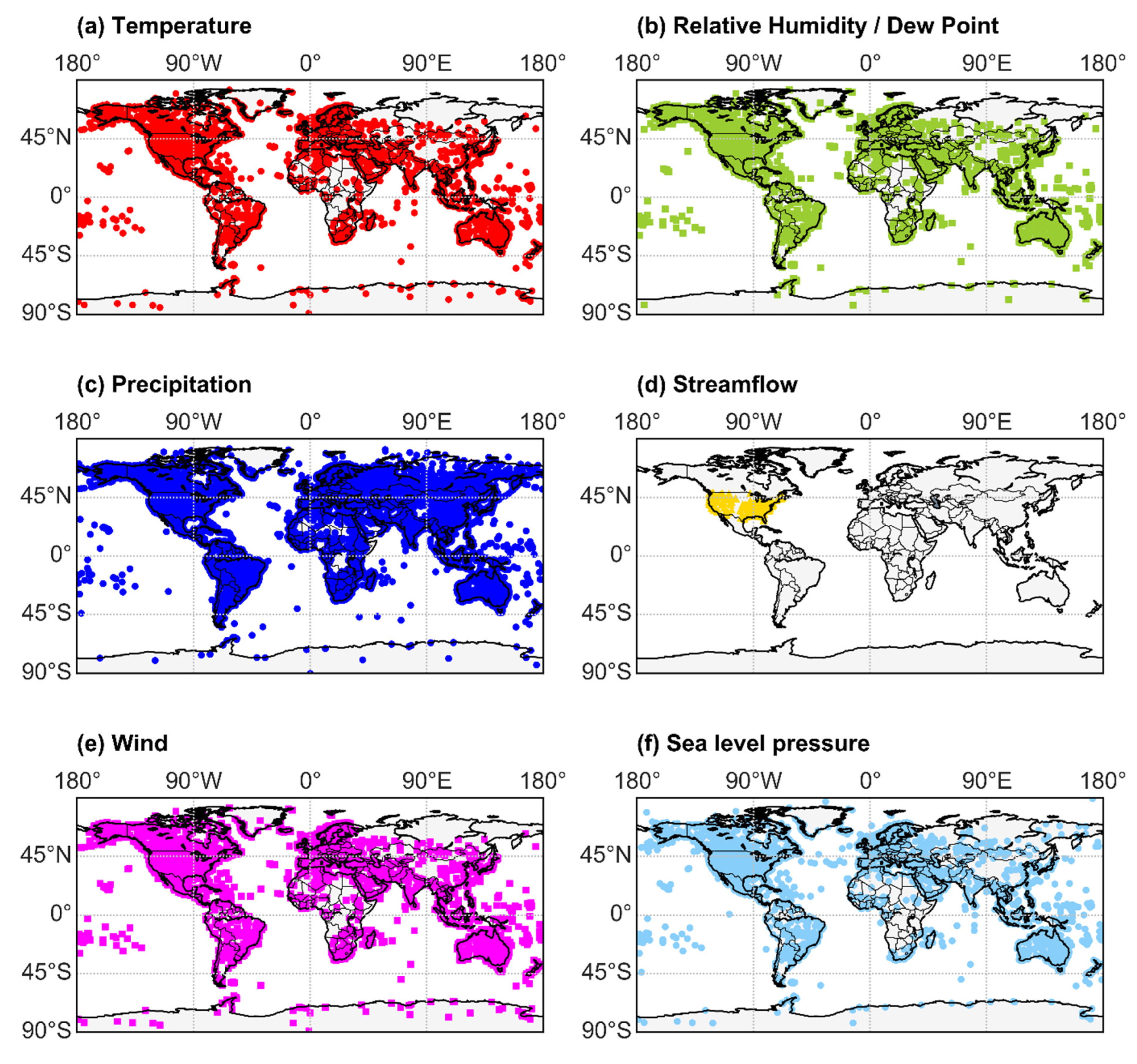
2.3. Global-Scale Data Extraction and Processing

The selected global-scale databases for the analysis after quality control are the ISD database [102,103,104,105,106,107,108,109,110,111] for near-surface hourly temperature, dew point, sea level pressure, and wind speed; the CAMELS database [112,113,114,115] for the daily streamflow; the USGS database [116] for the hourly streamflow; the GHCN database [117,118,119,120,121] for the daily precipitation; and the HPD database (https://www.ncei.noaa.gov/, lastly accessed on 15 December 2020) for the hourly precipitation. From the contained stations in each database, we selected stations with more than 5 years of full records (see Table 1 for more information on the selected stations, and Figure 1 for the visualization of their locations), and we discarded recordings that have quality flags. In addition, for other streamflow-related processes, we analyzed and discussed one of the largest daily discharge time series of the river Po [122] and the largest annual time series of the stage at the river Nile (e.g., [123]).
The relative humidity is estimated from the hourly temperature and dew point values as [124]:
U = ( T T d ) 5.06 e 24.921 T 0 ( T d T T d T )  
where U is the relative humidity (%); T and T d are the near-surface temperature and the dew point expressed in kelvin degrees, respectively; and T 0 = 273.16   K is the triple point of water.
To mitigate the effect that the periodicity of hydrological-cycle processes, prominent both in the diurnal and seasonal cycles (e.g., [125,126,127,128,129,130,131,132]), exerts on their modelling, we apply a double standardization on the processes with hourly resolution and a seasonal standardization on the ones with daily resolution. In particular, we subtract the mean from each periodicity cycle, and we divide with its standard deviation. In this way, although the effect of the double periodicity cannot be entirely removed, we diminish the propagation of its effect on the dependence structure. Moreover, to increase the available records in each cycle and the estimation accuracy, and without much affecting the dependence structure, we standardize each process based on a 6 hourly × 3 monthly resolution of the cycles, i.e., the diurnal periodicity is divided into 24/6 = 4 cycles, and the seasonal periodicity is divided also in 12/3 = 4 cycles.
In addition, the marginal and dependence structures of other key hydrological-cycle processes were included in the analysis, and the results from previous studies of global-scale stations or from the longest available samples worldwide were discussed. Specifically, these processes are the potential evapotranspiration [133,134], the solar radiation clearness index [62], and the ocean wind-wave height and period processes [135].
Finally, for the investigation of the stochastic similarities between the above key hydrological-cycle processes and the isotropic and nearly Gaussian turbulence, which resemble the turbulent shear and buoyancy in the atmospheric boundary layer, we show the results from a massive grid-turbulence database that includes 40 time series, each with 36 × 106 records of longitudinal wind velocity along the flow direction, all measured by X-wire probes placed downstream of the grid and in different positions, and with a sampling temporal resolution of 25 μs [136]. To shift from the spatial to the temporal domain [137], we apply a standardization to all time series by subtracting their mean and dividing by their standard deviation (see more information and results in [76]). In this manner, we may directly estimate the expected marginal and temporal dependence structure by combining the estimations from all the time series, approximately as if the same experiment was performed multiple times at the same position. For the buoyancy behavior, we discuss the results from several studies of Papanicolaou and List [138,139] and Dimitriadis et al. [18,140,141], where more than 10 time series of horizontal and vertical positively buoyant thermal jets of temperature concentration, recorded with the laser-induced-fluorescence technique, and with a 30 ms resolution, various nozzle diameters, discharges, initial and ambient temperature, and of more than 104 sample length each, were analyzed.

3. Results

The investigation of the marginal structure of the key hydrological-cycle processes is based here on the estimation of moments, and especially of high-order, which are indicative of the tail behavior. In this section, we present the results from the global-scale analysis, in terms of the second-order statistics, and particularly, the plots of the mean vs. standard deviation, of the skewness vs. kurtosis estimated from the C-, L-, K-moments, and of the climacogram and the climacospectrum (mean, and the 5% and 95% quantiles). Note that for the estimation of the model parameters adjusting for bias, we use scales up to 10% of the observation period for the climacogram (and thus, 5% for the CBS), in order not to use variance estimates from a sample size less than 10 [4].
In Figure 2, Figure 3, Figure 4, Figure 5, Figure 6, Figure 7 and Figure 8, which show the climacogram and climacospectrum for each process, we observed similarities in the shape of the dependence structure spanning from strong correlations at the small scales to a power-type behavior at large scales, with a convex-shape at the intermediate scales.
Although similarities may also be traced in the skewness–kurtosis plots, the more robust estimation of the L-skewness vs. L-kurtosis (Figure 9 and Figure 10) allows for more powerful comparisons. Still, the more advanced K-skewness and K-kurtosis estimations enable an even clearer view of the detected pattern in Figure 9 and Figure 11. Specifically, the K-skewness increases from the dew point to the humidity, to the temperature, sea level pressure, and grid turbulence, followed by a weaker increase of the K-kurtosis, while for the wind speed, streamflow, and precipitation processes, both the K-skewness and K-kurtosis highly increase. In addition, we observe how all sample K-skewness and K-kurtosis fall into the range of the mixed PBF distribution only by the analysis through K-moments. Finally, in Figure 12 and Figure 13, we observed that the dew point, relative humidity, temperature, and sea level pressure, along with grid turbulence, exhibit a stronger structure at the intermediate and large scales, followed by the wind speed, streamflow, and precipitation.
Therefore, this hierarchy of the key hydrological-cycle processes may be described by a transformation of the nearly Gaussian processes (i.e., dew point, humidity, temperature, and sea level pressure) with a stronger LTP dependence at large scales (H > 0.75) to the Pareto-type processes (i.e., wind speed, streamflow, and precipitation) with a weaker dependence LTP at larger scales (H ≤ 0.75). Interestingly, the same hierarchy is observed in a simplified cycle of the energy exchange among hydrological processes trough turbulent mixing, with the dew point, relative humidity, temperature, and sea level pressure, feeding the wind speed, while triggering precipitation, whose energy is then temporally stored in rivers and soil, and finally returned to the former processes through evaporation.
For the rest of the processes included in the current analysis, it was found that the clearness index of the solar radiation [62] and the ocean waves (height and period; [135]), as analyzed from the global databases mentioned above, exhibit a marginal structure similar to the sea level pressure and wind speed, respectively. In addition, they exhibit an HK dependence structure with H ≈ 0.8 and q ≈ 30 h, and H ≈ 0.9 and q ≈ 10 h, for the wave height and period, respectively, and H = 0.83 and q = 2 h for the clearness index of the solar radiation, while both having a fractal behavior with roughness (M < 0.5). The standardized temperature concentration of the turbulent buoyant jet along the axis [141], is found to exhibit similar behavior as in the grid turbulence with a nearly Gaussian marginal structure, and a rough (M < 0.5, at small scales) and strong LTP (H > 0.6, at the jet-like area and H > 0.9 at the plume-like area) dependence structure. Finally, the evapotranspiration process was also found to exhibit a weak LTP behavior (H ≈ 0.6) and a similar marginal structure to temperature and solar radiation [133,134].
Finally, the summary statistics from the global-scale analysis can be seen in Table 2 and Table 3, where the mean from the C-, L-, and K-moments as well as the scale, fractal, Hurst, and scale parameter of the expected second-order dependence structure, respectively, were estimated and are discussed in more detail at the next section. It is noted that merger of the time series of a different resolution, such as in streamflow and precipitation, was performed after adjusting for bias (see more details from a similar global-scale analysis of fine-resolution and large-scale temperature and wind in [70]).

4. Discussion

The investigation of the uncertainty in the hydrological cycle is an important scientific field, as recognized by the International Association of Hydrological Sciences (IAHS) by launching the Panta Rhei research initiative for the Scientific Decade 2013–2022 [142].
An overall conclusion from this study is that the Hurst parameter is estimated significantly above 0.5 for all processes (Table 3 and Figure 12 and Figure 13), indicating that the observed uncertainty and climatic variability in the hydrological cycle may be caused by the presence of the long-term persistent (LTP) behavior (see also discussion in [143,144]). This is consistent with the universality of LTP behavior as confirmed in various other studies (than the ones mentioned in Section 2.1) and statistical attributes in literature (for a review see [18,145,146,147]), such as in global-scale key hydrometeorological processes [3,18], trend analysis [148] and extremes [149,150], precipitation [151,152,153,154,155], streamflow [155,156,157], turbulent jets [158,159] and grid turbulence [160,161].
The intermediate scale behavior of the dependence structure (Table 3 and Figure 13), which was found to be consistent with the K41 law of Kolmogorov [162,163] for all processes, corresponds to a fractal parameter of M = 1/3 (i.e., roughness behavior of M < 0.5). For even smaller scales, the fractal parameter was estimated even lower or close-to-zero for all the examined processes. However, for the more robust estimation of the fractal parameter, additional data and of higher resolution are required. For example, in [70], where high resolution samples (of 10 Hz) were applied to the temperature and wind speed, the fractal parameter was estimated in both processes as M ≈ 1/3. It is noted that in the multifractal analysis, the change of the dependence structure is viewed as a scale break, and similar positions of the break is identified in the intermediate scales of streamflow and precipitation in the analyses [164,165,166,167,168,169].
In terms of the marginal structure, our results are consistent with other global-scale studies in literature (besides the ones previously mentioned in Section 2.2) on nearly Gaussian temperature [89], wind speed transition of extreme tail from Rayleigh to Weibull and Pareto-type [70,170,171,172], sea level pressure [173], streamflow heavy tail [157,174], precipitation Pareto-type tail [3,74,149,175,176,177,178,179,180,181,182], evaporation [183,184], and nearly Gaussian turbulent processes [185].
The high uncertainty of geophysical dynamics is linked to the power-law type of the marginal distribution as well as of the dependence structure through empirical evidence and physical justification. Although the above and other studies have focused on one or a limited number of processes, in this study we analyze several key hydrological-cycle processes, namely near-surface temperature, dew point, humidity, sea level pressure, atmospheric wind speed, streamflow, precipitation, as well as other processes from previous studies, such as solar radiation clearness index and ocean waves, where we trace stochastic similarities in their marginal and dependence structures. Moreover, we find similar stochastic structures in turbulent shear and buoyancy processes, as studied through laboratory records of grid-turbulent wind speeds and temperature concentrations of buoyant turbulent jets along the axis.
Specifically, a hierarchy emerges (a) for the marginal structure visualized through the skewness–kurtosis plot, both estimated through the K-moments, while similar but weaker empirical conclusions can be derived by the plot of the C-moments and L-moments; and (b) for the dependence structure visualized through the climacogram and climacospectrum. This hierarchy starts with temperature, dew point, relative humidity, solar radiation index, evaporation, and sea level pressure, all of which exhibit a stronger skewness over kurtosis absolute ratio than the turbulent processes, wind speed, and ocean waves. All the latter processes exhibit a stronger LTP behavior in the dependence structure, whereas streamflow and precipitation present a weaker skewness over kurtosis absolute ratio and an LTP behavior.
Interestingly, the same hierarchy is observed in the energy exchange among processes in the hydrological cycle. It starts with the solar radiation, temperature, dew point (or equivalently, relative humidity), and sea level pressure. These feed the wind speed and ocean waves through nearly Gaussian and isotropic turbulent mixing in the boundary layer. Next, they trigger precipitation, which then moves to streams and soil, and is finally returned to the former processes through evaporation.

5. Conclusions

The major innovation of this study is the uniting view of the key hydrological-cycle processes through the analysis of several billions of observations from hundred thousands of stations by robust statistical metrics of (a) the K-moments, for the estimation of the marginal structure of the first four moments, and of (b) the climacogram, for the estimation of the second-order dependence structure. The key examined hydrological-cycle processes are the near-surface temperature, dew point, humidity, sea level pressure, atmospheric wind speed, streamflow, and precipitation, as well as other processes from previous studies, such as shear and buoyant turbulent processes analyzed through small-scale laboratory experiments, and solar radiation, and ocean waves. The main traced stochastic similarities are as follows:
(1)
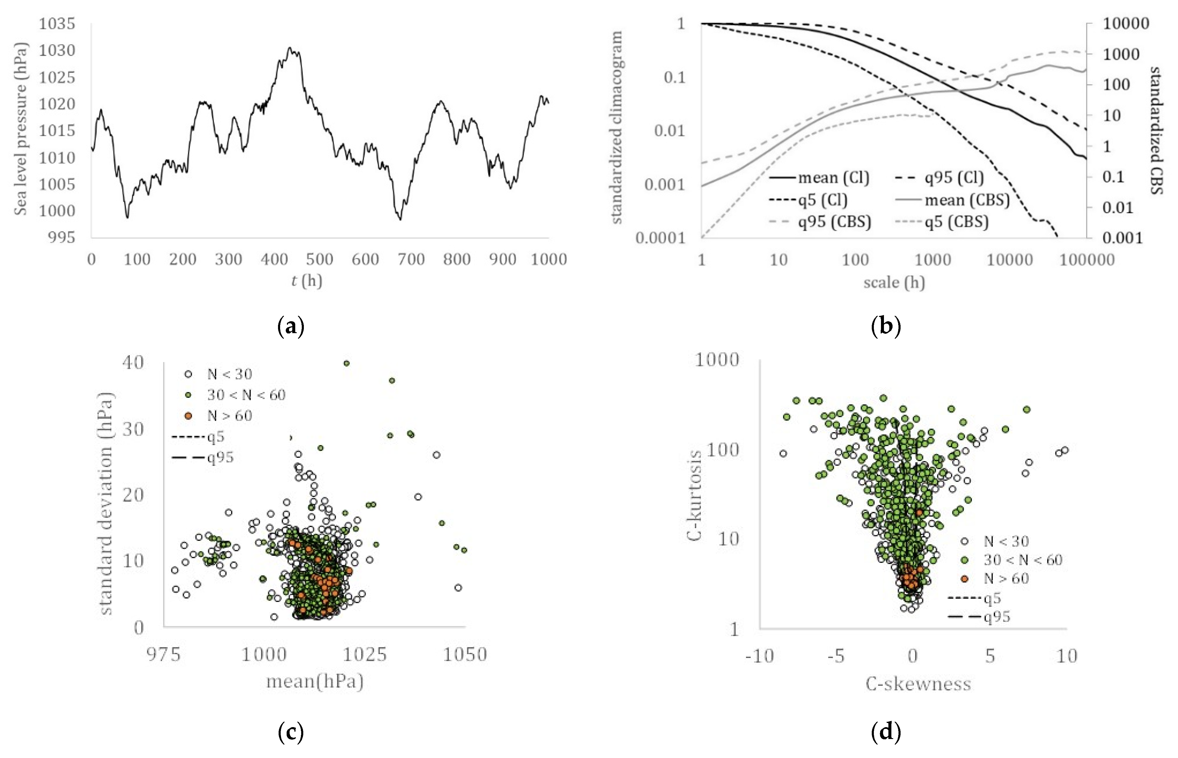
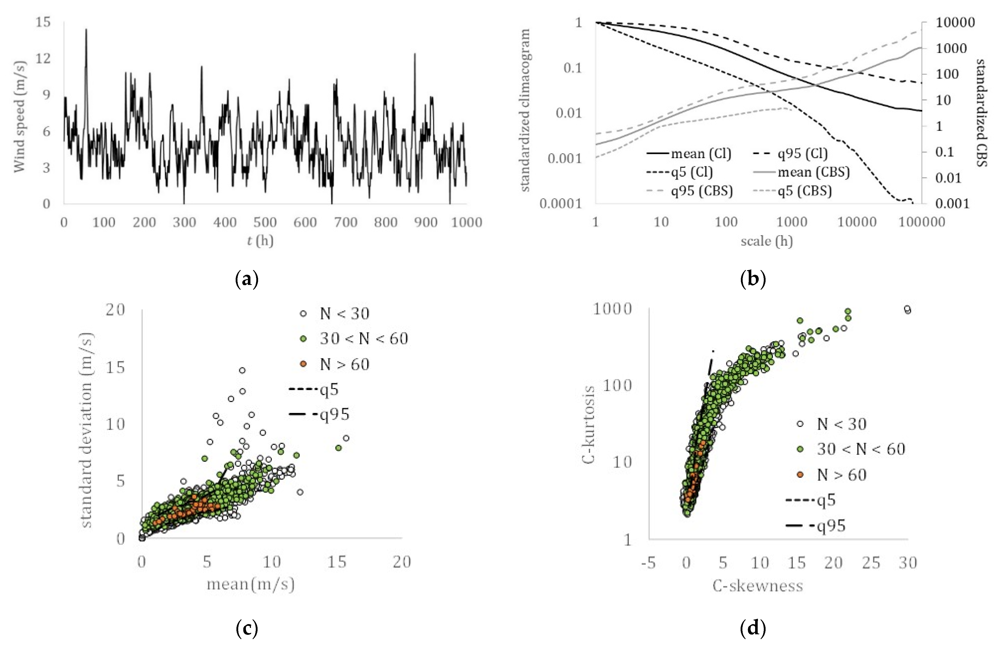
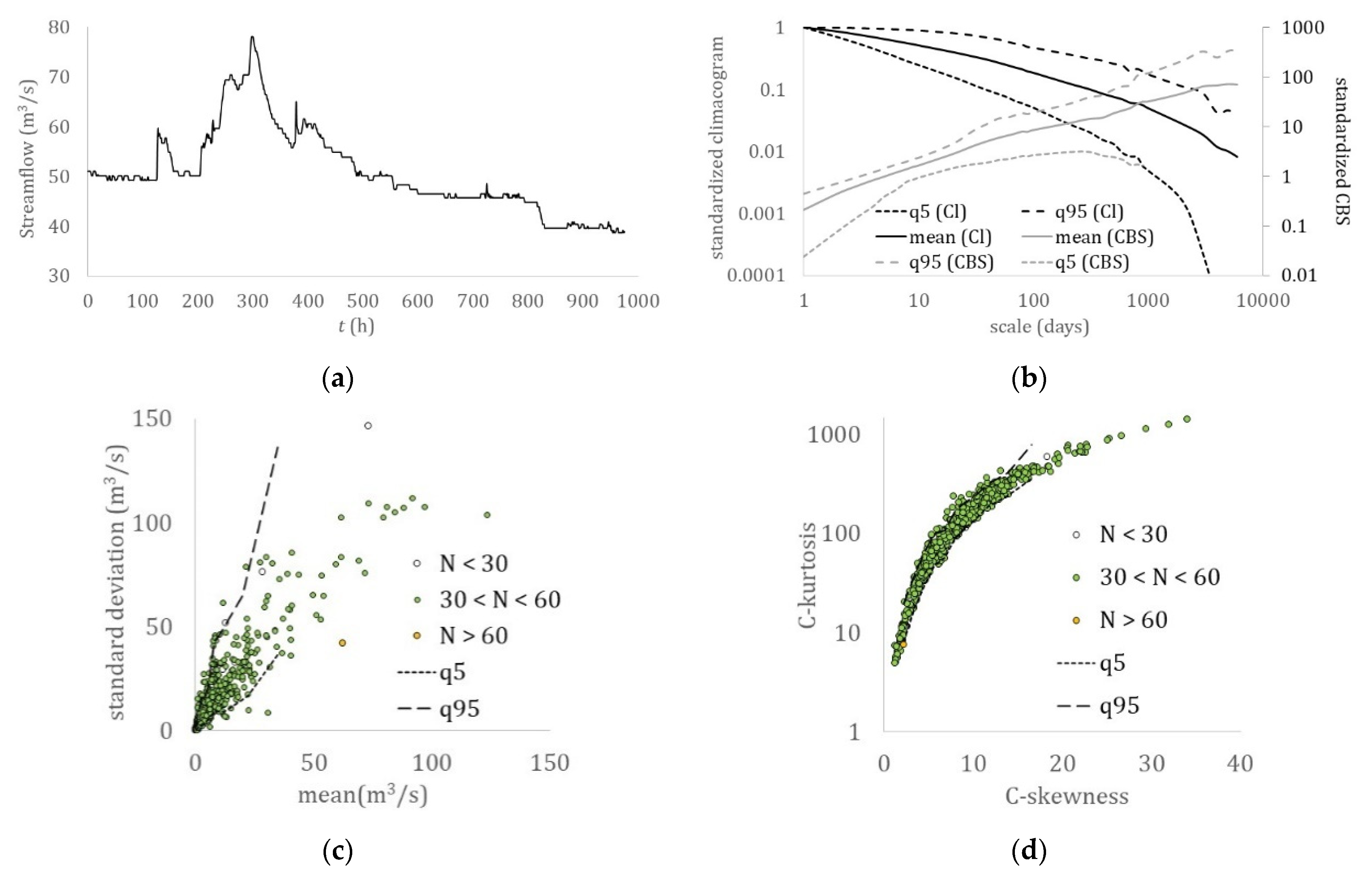
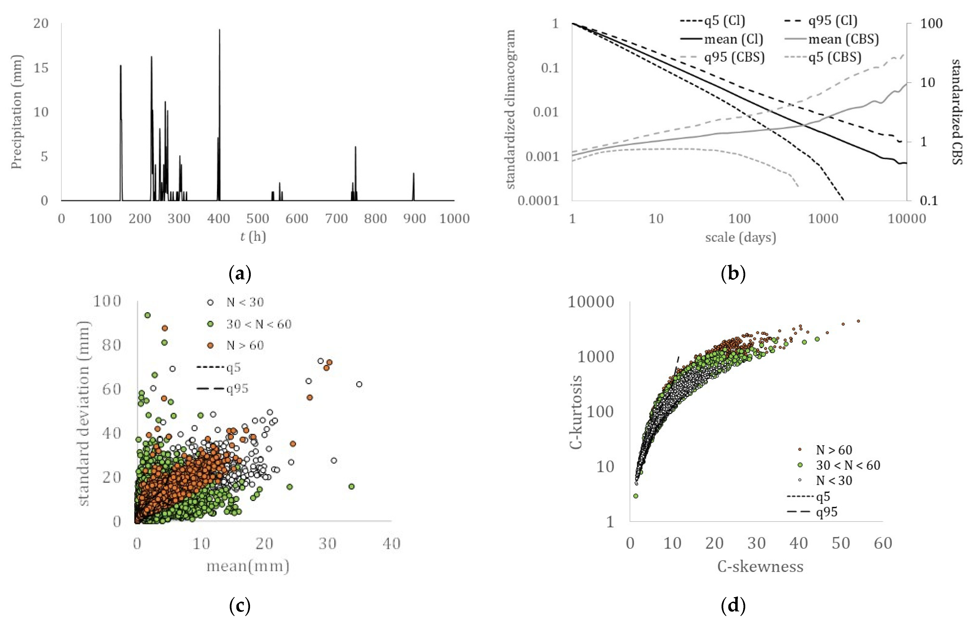
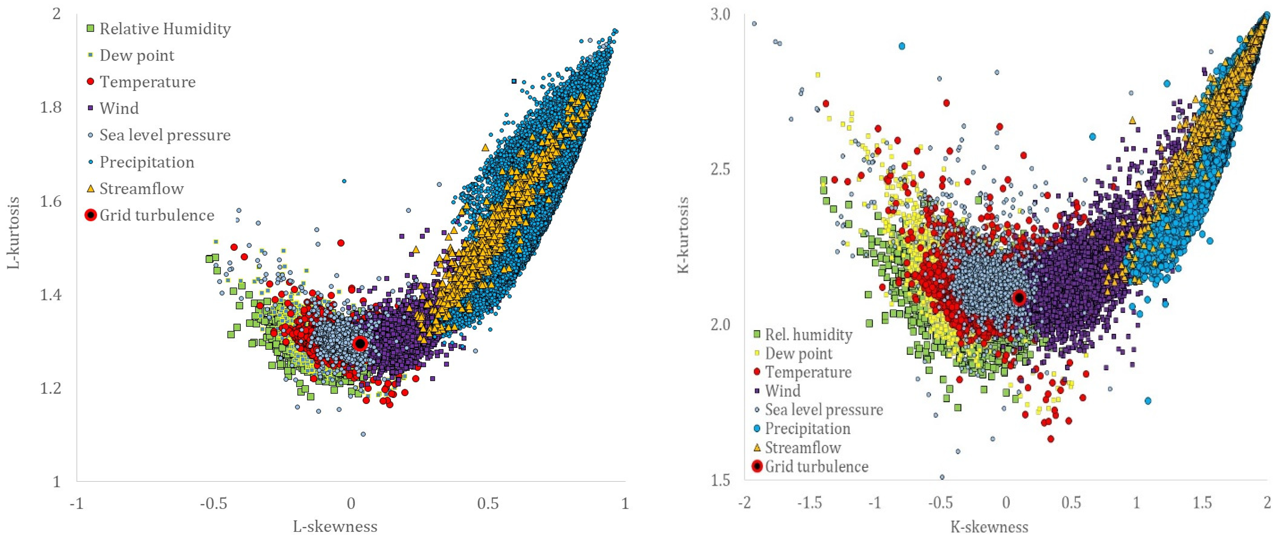
A hierarchy related to the hydrological cycle was identified with the dew point, temperature, relative humidity, solar radiation, and sea level pressure all exhibiting a lower skewness over kurtosis absolute ratio than the turbulent processes, wind speed, and ocean waves, and with a stronger long-term persistence (LTP) behavior in the dependence structure (H > 0.75), followed by streamflow and precipitation, both of which exhibit a smaller skewness–kurtosis absolute ratio and a weaker LTP behavior (H ≤ 0.75).
(2)
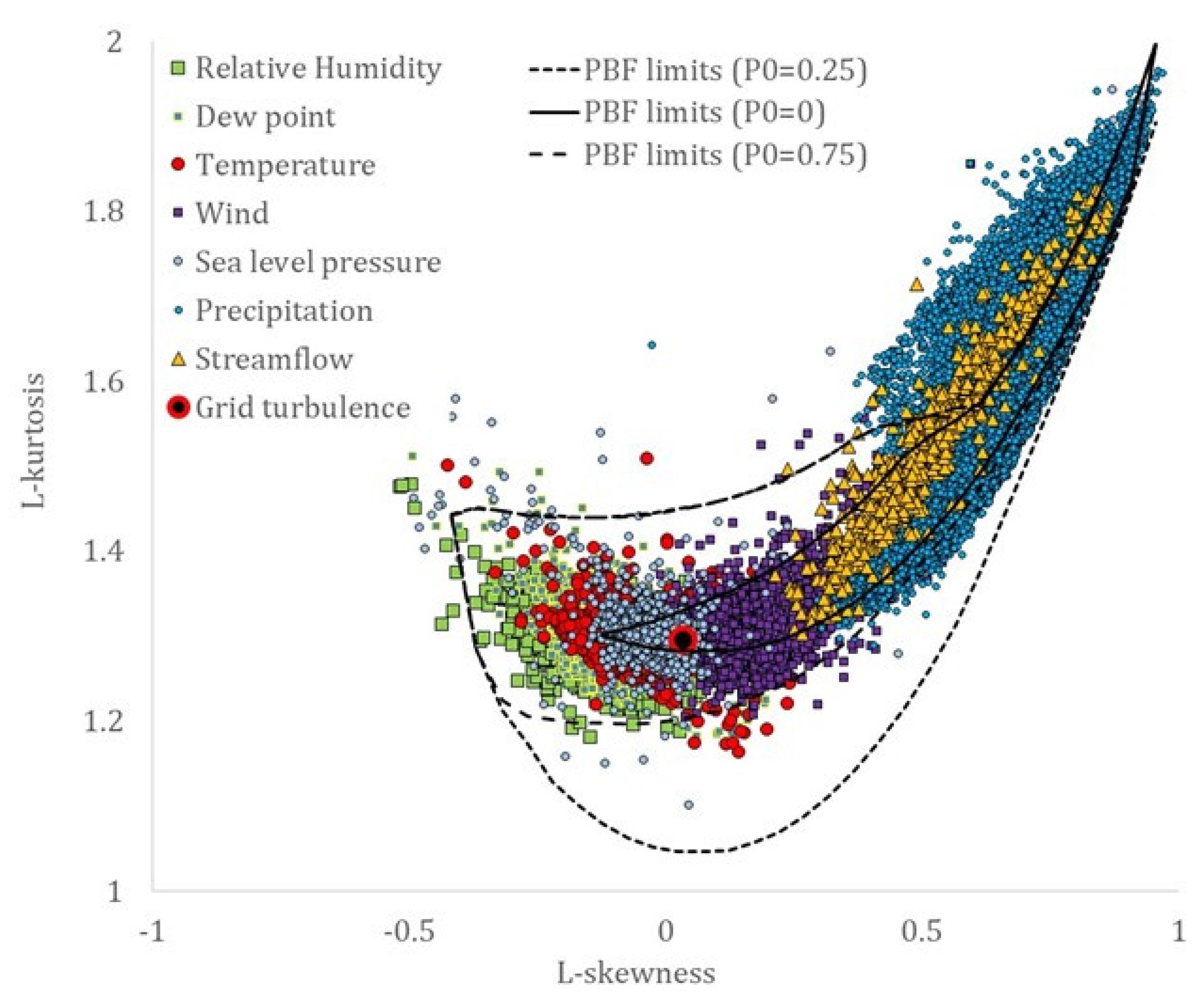
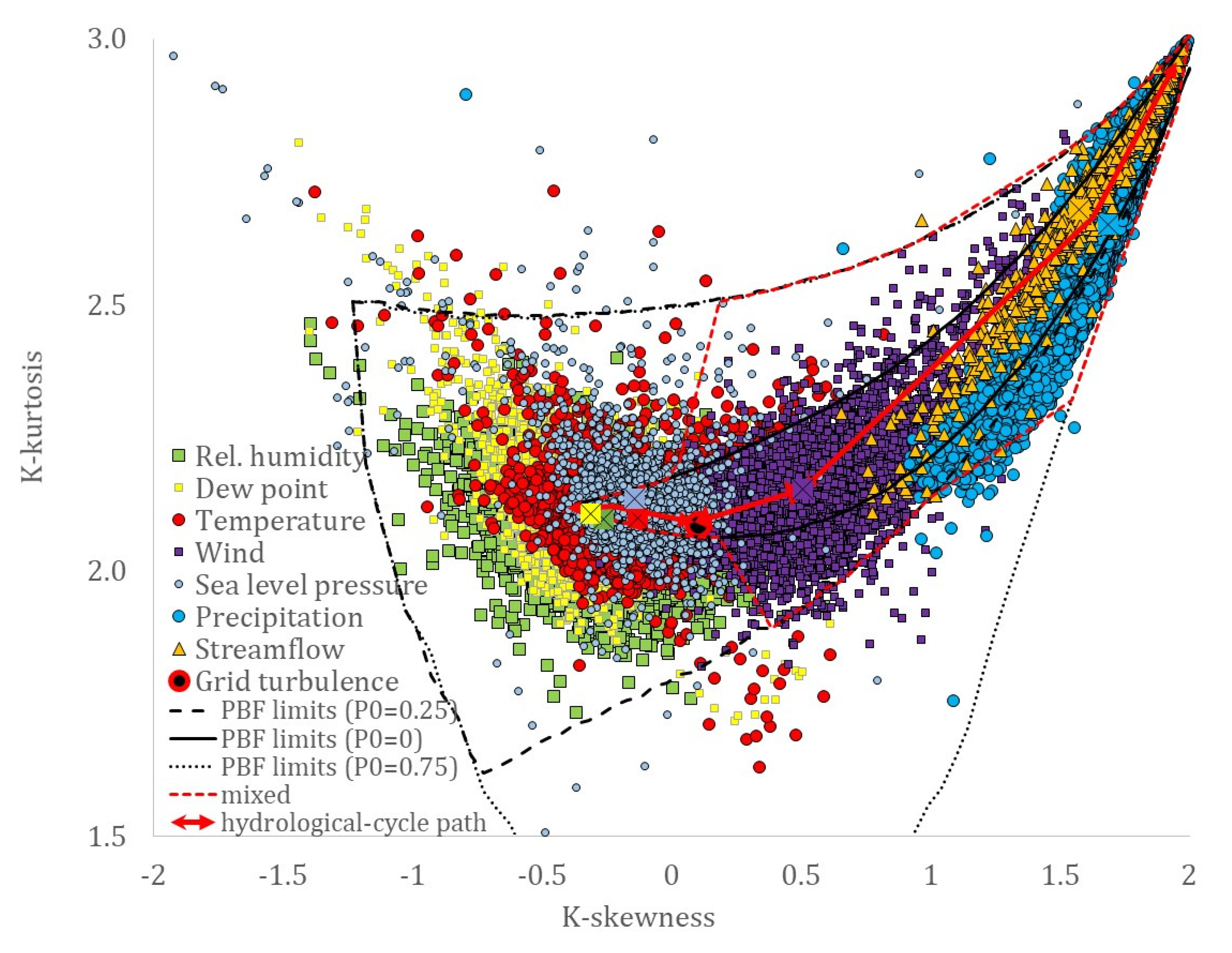
All the examined processes can be adequately simulated by the truncated mixed-PBF distribution, adjusting for probability dry and lower (or upper) truncation, in terms of the first four moments, and ranging from (truncated) nearly Gaussian to Pareto-type tails.
(3)
As the sample size increases, different records of the same process from several locations converge to a smaller area of the nondimensionalized statistics (skewness–kurtosis), indicating a common marginal behavior.
(4)
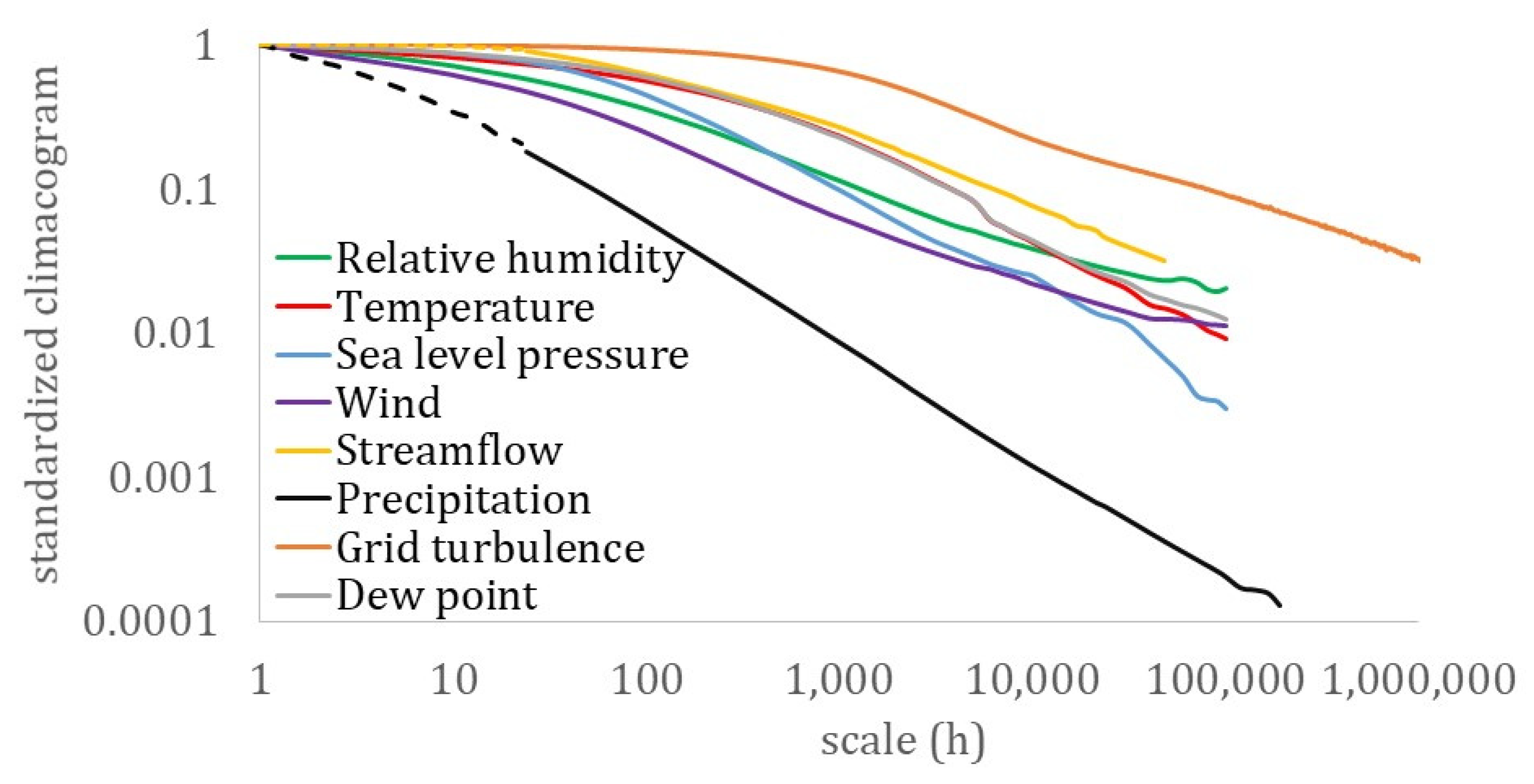
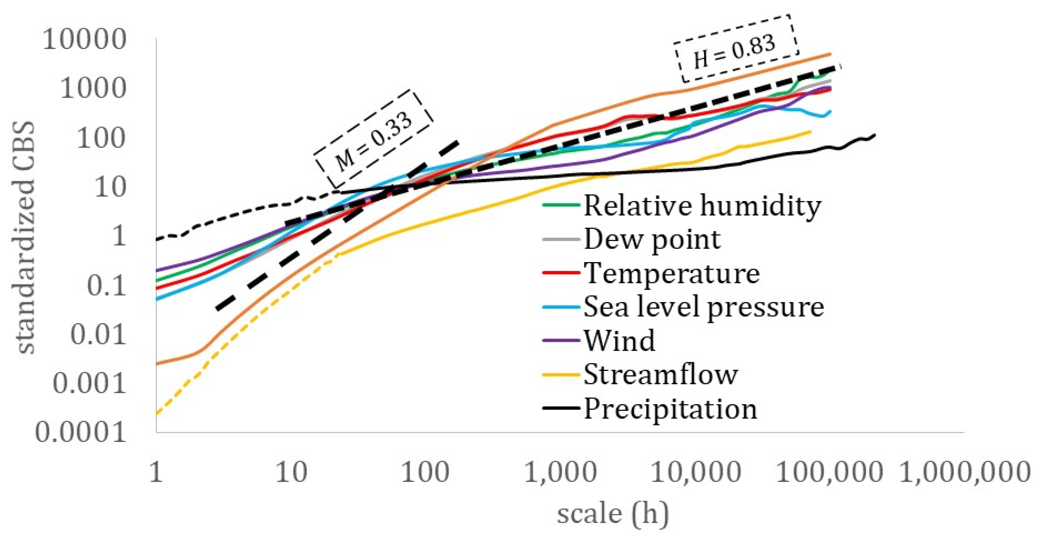
All the examined hydrological-cycle processes exhibit a similar dependence structure that extends from the fractal behavior with roughness (M < 0.5) located at the small-intermittent scales to the LTP behavior at large scales (H > 0.5), while both indicate large uncertainty and high climatic variability.
(5)
Finally, since the above empirical findings are consistent with previous studies and can be justified by the principle of maximum entropy, they allow for a uniting stochastic view of the hydrological-cycle processes under the Hurst–Kolmogorov (HK) dynamics in terms of both the marginal and dependence structures.

Author Contributions

Conceptualization, P.D., D.K., T.I., P.P.; Formal analysis, P.D., D.K., T.I., P.P.; Methodology, P.D., D.K., T.I., P.P.; Resources, P.D. and T.I.; Supervision, D.K. and P.P.; Validation, P.D., D.K., T.I., P.P.; Visualization, P.D., D.K., T.I., P.P.; Writing—original draft, P.D.; Writing—review & editing, D.K., T.I., P.P. All authors have read and agreed to the published version of the manuscript.

Funding

This research is carried out/funded in the context of the project “Development of Stochastic Methods for Extremes (ASMA): identification and simulation of dependence structures of extreme hydrological events” (MIS 5049175) under the call for proposals “Researchers’ support with an emphasis on young researchers—2nd Cycle”. The project is co-financed by Greece and the European Union (European Social Fund; ESF) by the Operational Programme Human Resources Development, Education, and Lifelong Learning 2014–2020.
Hydrology 08 00059 i001

Acknowledgments

We thank the anonymous reviewers, and the academic and assistant editors’ fruitful comments and handling of the manuscript.

Conflicts of Interest

The authors declare no conflict of interest.

References

  1. Poincaré, H. Sur le probleme des trois corps et les équations de la dynamique. Acta Math. 1890, 13, A3–A270. [Google Scholar]
  2. Lorenz, E.N. Deterministic nonperiodic flow. J. Atmospheric Sci. 1963, 20, 130–141. [Google Scholar] [CrossRef] [Green Version]
  3. Koutsoyiannis, D. Stochastics of Hydroclimatic Extremes—A Cool Look at Risk; Edition 0; National Technical University of Athens: Athens, Greece, 2021; 330p. [Google Scholar]
  4. Dimitriadis, P.; Koutsoyiannis, D. Climacogram versus autocovariance and power spectrum in stochastic modelling for Markovian and Hurst–Kolmogorov processes. Stoch. Environ. Res. Risk Assess. 2015, 29, 1649–1669. [Google Scholar] [CrossRef]
  5. Falkovich, G.; Fouxon, A.; Stepanov, M.G. Acceleration of rain initiation by cloud turbulence. Nat. Cell Biol. 2002, 419, 151–154. [Google Scholar] [CrossRef]
  6. Langousis, A.; Veneziano, D. Long-term rainfall risk from tropical cyclones in coastal areas. Water Resour. Res. 2009, 45. [Google Scholar] [CrossRef] [Green Version]
  7. Wilson, J.D.; Sawford, B.L. Review of Lagrangian stochastic models for trajectories in the turbulent atmosphere. Bound. Layer Meteorol. 1996, 78, 191–210. [Google Scholar] [CrossRef]
  8. Ghannam, K.; Katul, G.G.; Bou-Zeid, E.; Gerken, T.; Chamecki, M. Scaling and Similarity of the Anisotropic Coherent Eddies in Near-Surface Atmospheric Turbulence. J. Atmospheric Sci. 2018, 75, 943–964. [Google Scholar] [CrossRef]
  9. Ayet, A.; Katul, G.G.; Bragg, A.D.; Redelsperger, J.L. Scalewise Return to Isotropy in Stratified Boundary Layer Flows. J. Geophys. Res. Atmos. 2020, 125. [Google Scholar] [CrossRef]
  10. Hurst, H.E. Long-Term Storage Capacity of Reservoirs. Trans. Am. Soc. Civ. Eng. 1951, 116, 770–799. [Google Scholar] [CrossRef]
  11. Kolmogorov, A.N. Wiener Spirals and Some Other Interesting Curves in a Hilbert Space; Selected Works of Mathematics and Mechanics; Kolmogorov, A.N., Tikhomirov, V.M., Eds.; Kluwer: Dordrecht, The Netherlands, 1991; pp. 303–307. [Google Scholar]
  12. Mandelbrot, B.B. A Fast Fractional Gaussian Noise Generator. Water Resour. Res. 1971, 7, 543–553. [Google Scholar] [CrossRef]
  13. Koutsoyiannis, D. HESS opinions, A random walk on water. Hydrol. Earth Syst. Sci. 2010, 14, 585–601. [Google Scholar] [CrossRef] [Green Version]
  14. Koutsoyiannis, D. Hurst–Kolmogorov dynamics as a result of extremal entropy production. Phys. A: Stat. Mech. its Appl. 2011, 390, 1424–1432. [Google Scholar] [CrossRef]
  15. Koutsoyiannis, D. Hurst-Kolmogorov dynamics and uncertainty. J. Am. Water Resourc. Assoc. 2011, 47, 481–495. [Google Scholar] [CrossRef]
  16. Koutsoyiannis, D. Entropy: From Thermodynamics to Hydrology. Entropy 2014, 16, 1287–1314. [Google Scholar] [CrossRef] [Green Version]
  17. Koutsoyiannis, D. Entropy Production in Stochastics. Entropy 2017, 19, 581. [Google Scholar] [CrossRef] [Green Version]
  18. Dimitriadis, P. Hurst-Kolmogorov Dynamics in Hydrometeorological Processes and in the Microscale of Turbulence. Ph.D. Thesis, National Technical University of Athens, Athens, Greece, 2017; 167p. [Google Scholar]
  19. Koutsoyiannis, D. The Hurst phenomenon and fractional Gaussian noise made easy. Hydrol. Sci. J. 2002, 47, 573–595. [Google Scholar] [CrossRef]
  20. Koutsoyiannis, D. Generic and parsimonious stochastic modelling for hydrology and beyond. Hydrol. Sci. J. 2016, 61, 225–244. [Google Scholar] [CrossRef]
  21. Koutsoyiannis, D. A generalized mathematical framework for stochastic simulation and forecast of hydrologic time series. Water Resour. Res. 2000, 36, 1519–1533. [Google Scholar] [CrossRef] [Green Version]
  22. Koutsoyiannis, D. Time’s arrow in stochastic characterization and simulation of atmospheric and hydrological processes. Hydrol. Sci. J. 2019, 64, 1013–1037. [Google Scholar] [CrossRef]
  23. Koutsoyiannis, D. Simple stochastic simulation of time irreversible and reversible processes. Hydrol. Sci. J. 2020, 65, 536–551. [Google Scholar] [CrossRef]
  24. Lombardo, F.; Volpi, E.; Koutsoyiannis, D. Rainfall downscaling in time: Theoretical and empirical comparison between multifractal and Hurst-Kolmogorov discrete random cascades. Hydrol. Sci. J. 2012, 57, 1052–1066. [Google Scholar] [CrossRef] [Green Version]
  25. Efstratiadis, A.Y.; Dialynas, S.; Kozanis; Koutsoyiannis, D. A multivariate stochastic model for the generation of synthet-ic time series at multiple time scales reproducing long-term persistence. Environ. Model. Softw. 2014, 62, 139–152. [Google Scholar] [CrossRef]
  26. Dimitriadis, P.; Koutsoyiannis, D. Stochastic synthesis approximating any process dependence and distribution. Stoch. Environ. Res. Risk Assess. 2018, 32, 1493–1515. [Google Scholar] [CrossRef]
  27. Kossieris, P.; Makropoulos, C.; Onof, C.; Koutsoyiannis, D. A rainfall disaggregation scheme for sub-hourly time scales: Coupling a Bartlett-Lewis based model with adjusting procedures. J. Hydrol. 2018, 556, 980–992. [Google Scholar] [CrossRef] [Green Version]
  28. Papalexiou, S.M.; Markonis, Y.; Lombardo, F.; AghaKouchak, A.; Foufoula-Georgiou, E. Precise Temporal Disaggregation Preserving Marginals and Correlations (DiPMaC) for Stationary and Nonstationary Processes. Water Resour. Res. 2018, 54, 7435–7458. [Google Scholar] [CrossRef]
  29. Papalexiou, S.M.; Serinaldi, F. Random Fields Simplified: Preserving Marginal Distributions, Correlations, and Intermittency, With Applications from Rainfall to Humidity. Water Resour. Res. 2020, 56. [Google Scholar] [CrossRef] [Green Version]
  30. Tsoukalas, I.; Makropoulos, C.; Koutsoyiannis, D. Simulation of Stochastic Processes Exhibiting Any-Range Dependence and Arbitrary Marginal Distributions. Water Resour. Res. 2018, 54, 9484–9513. [Google Scholar] [CrossRef]
  31. Tsoukalas, I.; Kossieris, P.; Makropoulos, C. Simulation of Non-Gaussian Correlated Random Variables, Stochastic Processes and Random Fields: Introducing the anySim R-Package for Environmental Applications and beyond. Water 2020, 12, 1645. [Google Scholar] [CrossRef]
  32. Papoulis, A.; Pillai, S.U. Stochastic Processes; McGraw-Hill: New York, NY, USA, 1991. [Google Scholar]
  33. Lombardo, F.C.; Volpi, E.; Koutsoyiannis, D.; Papalexiou, S.M. Just two moments! A cautionary note against use of high-order moments in multifractal models in hydrology. Hydrol. Earth Syst. Sci. 2014, 18, 243–255. [Google Scholar] [CrossRef] [Green Version]
  34. Geweke, J.; Porter-Hudak, S. The estimation and application of long memory time series models. J. Time Ser. Anal. 1983, 4, 221–238. [Google Scholar] [CrossRef]
  35. Beran, J. Statistical Methods for Data with Long-Range Dependence. Stat. Sci. 1992, 7, 404–416. [Google Scholar]
  36. Beran, J. Estimation, Testing and Prediction for Self-Similar and Related Processes. Ph.D. Thesis, ETH, Zurich, Switzerland, 1986. [Google Scholar]
  37. Mandelbrot, B.B.; Wallis, J.R. Noah, Joseph and operational hydrology. Water Resour. Res. 1968, 4, 909–918. [Google Scholar] [CrossRef] [Green Version]
  38. Granger, C.W.J.; Joyeux, R. An Introduction to Long-memory Time Series, Models and Fractional Differencing. J. Time Ser. Anal. 1980, 1, 15–29. [Google Scholar] [CrossRef]
  39. Koutsoyiannis, D. Climate change impacts on hydrological science: A comment on the relationship of the climacogram with Allan variance and variogram. ResearchGate 2018. [Google Scholar] [CrossRef]
  40. Smith, F.H. An empirical law describing heterogeneity in the yields of agricultural crops. Agric. Sci. 1938, 28, 1–23. [Google Scholar] [CrossRef]
  41. Cox, D.R. Long-Range Dependence: A review, Statistics: An Appraisal. In Proceedings of the 50th Anniversary Conference; David, H.A., David, H.T., Eds.; Iowa State University Press: Iowa City, IA, USA, 1984; pp. 55–74. [Google Scholar]
  42. Beran, J. A Test of Location for Data with Slowly Decaying Serial Correlations. Biometrika 1989, 76, 261. [Google Scholar] [CrossRef]
  43. Beran, J. Statistical Aspects of Stationary Processes with Long-Range Dependence; Mimeo Series 1743; Department Statistics University: Chapel Hill, NC, USA, 1988. [Google Scholar]
  44. Montanari, A.; Rosso, R.; Taqqu, M.S. Fractionally differenced ARIMA models applied to hydrologic time series: Identification, estimation, and simulation. Water Resour. Res. 1997, 33, 1035–1044. [Google Scholar] [CrossRef]
  45. Montanari, A.; Taqqu, M.S.; Teverovsky, V. Estimating long-range dependence in the presence of periodicity: An empiri-cal study. Math. Comput. Modeling 1999, 29, 217–228. [Google Scholar] [CrossRef]
  46. Koutsoyiannis, D. Hydrologic Persistence and the Hurst Phenomenon, Water Encyclopedia; Surface and Agricultural Water; Lehr, J.H., Keeley, J., Eds.; Wiley: New York, NY, USA, 2005; Volume 4, pp. 210–221. [Google Scholar] [CrossRef]
  47. Koutsoyiannis, D. Climate change, the Hurst phenomenon, and hydrological statistics. Hydrol. Sci. J. 2003, 48, 3–24. [Google Scholar] [CrossRef]
  48. Tyralis, H.; Koutsoyiannis, D. Simultaneous estimation of the parameters of the Hurst–Kolmogorov stochastic process. Stoch. Environ. Res. Risk Assess. 2010, 25, 21–33. [Google Scholar] [CrossRef]
  49. Koutsoyiannis, D. Encolpion of Stochastics: Fundamentals of Stochastic Processes; Department of Water Resources and Environmental Engineering—National Technical University of Athens: Athens, Greece, 2013. [Google Scholar] [CrossRef]
  50. Koutsoyiannis, D.; Paschalis, A.; Theodoratos, N. Two-dimensional Hurst–Kolmogorov process and its application to rainfall fields. J. Hydrol. 2011, 398, 91–100. [Google Scholar] [CrossRef]
  51. Dimitriadis, P.; Koutsoyiannis, D.; Onof, C. N-Dimensional generalized Hurst-Kolmogorov process and its application to wind fields. In Proceedings of the Facets of Uncertainty: 5th EGU Leonardo Conference—Hydrofractals 2013—STAHY 2013, Kos Island, Greece, 17–19 October 2013; European Geosciences Union, International Association of Hydrological Sciences. International Union of Geodesy and Geophysics: Prague, Czech Republic, 2013. [Google Scholar] [CrossRef]
  52. Koutsoyiannis, D. Hydrology and Change. Hydrol. Sci. J. 2013, 58, 1177–1197. [Google Scholar] [CrossRef]
  53. Markonis, Y.; Koutsoyiannis, D. Climatic Variability over Time Scales Spanning Nine Orders of Magnitude: Connecting Milankovitch Cycles with Hurst–Kolmogorov Dynamics. Surv. Geophys. 2012, 34, 181–207. [Google Scholar] [CrossRef]
  54. Markonis, Y.; Koutsoyiannis, D. Scale-dependence of persistence in precipitation records. Nat. Clim. Chang. 2015, 6, 399–401. [Google Scholar] [CrossRef]
  55. Tyralis, H.; Koutsoyiannis, D. A Bayesian statistical model for deriving the predictive distribution of hydroclimatic varia-bles. Clim. Dyn. 2014, 42, 2867–2883. [Google Scholar] [CrossRef]
  56. Iliopoulou, T.S.M.; Papalexiou, Y.; Markonis; Koutsoyiannis, D. Revisiting long-range dependence in annual precipita-tion. J. Hydrol. 2018, 556, 891–900. [Google Scholar] [CrossRef]
  57. Kossieris, P.; Tsoukalas, I.; Makropoulos, C.; Savic, D. Simulating Marginal and Dependence Behaviour of Water Demand Processes at Any Fine Time Scale. Water 2019, 11, 885. [Google Scholar] [CrossRef] [Green Version]
  58. Serinaldi, F.; Kilsby, C.G. Understanding Persistence to Avoid Underestimation of Collective Flood Risk. Water 2016, 8, 152. [Google Scholar] [CrossRef] [Green Version]
  59. Serinaldi, F. Can we tell more than we can know? The limits of bivariate drought analyses in the United States. Stoch. Environ. Res. Risk Assess. 2015, 30, 1691–1704. [Google Scholar] [CrossRef]
  60. Tsekouras, G.; Koutsoyiannis, D. Stochastic analysis and simulation of hydrometeorological processes associated with wind and solar energy. Renew. Energy 2014, 63, 624–633. [Google Scholar] [CrossRef]
  61. Mamassis, N.; Efstratiadis, A.; Dimitriadis, P.; Iliopoulou, T.; Ioannidis, R.; Koutsoyiannis, D. Water and Energy, Handbook of Water Resources Management: Discourses, Concepts and Examples; Bogardi, J.J., Tingsanchali, T., Nandalal, K.D.W., Gupta, J., Salamé, L., van Nooijen, R.R.P., Kolechkina, A.G., Kumar, N., Bhaduri, A., Eds.; Springer Nature: Cham, Switzerland, 2021; Chapter 20; pp. 617–655. [Google Scholar] [CrossRef]
  62. Koudouris, G.P.; Dimitriadis, T.; Iliopoulou, N.; Mamassis; Koutsoyiannis, D. A stochastic model for the hourly solar ra-diation process for application in renewable resources management. Adv. Geosci. 2018, 45, 139–145. [Google Scholar] [CrossRef] [Green Version]
  63. Moschos, E.; Manou, G.; Dimitriadis, P.; Afendoulis, V.; Koutsoyiannis, D.; Tsoukala, V. Harnessing wind and wave resources for a Hybrid Renewable Energy System in remote islands: a combined stochastic and deterministic approach. Energy Proc. 2017, 125, 415–424. [Google Scholar] [CrossRef]
  64. Aguilar, C.; Montanari, A.; Polo, M.-J. Real-time updating of the flood frequency distribution through data assimilation. Hydrol. Earth Syst. Sci. 2017, 21, 3687–3700. [Google Scholar] [CrossRef] [Green Version]
  65. Giglioni, M.; Lombardo, F.; Mineo, C. Investigating the Hurst-Kolmogorov Behavior of Sicily’s Climatological Time Series. In Proceedings of the International Conference of Numerical Analysis and Applied Mathematics (ICNAAM 2016), Rhodes, Greece, 19–25 September 2016; AIP Publishing: College Park, MD, USA, 2017; Volume 470004. [Google Scholar]
  66. Markonis, Y.Y.; Moustakis, C.; Nasika, P.; Sychova, P.; Dimitriadis, M.; Hanel, P.; Máca; Papalexiou, S.M. Global estima-tion of long-term persistence in annual river runoff. Adv. Water Resour. 2018, 113, 1–12. [Google Scholar] [CrossRef]
  67. Pappas, C.M.D.; Mahecha, D.C.; Frank, F.; Babst; Koutsoyiannis, D. Ecosystem functioning is enveloped by hydromete-orological variability. Nature Ecol. Evol. 2017, 1, 1263–1270. [Google Scholar] [CrossRef] [Green Version]
  68. Dimitriadis, P.; Tzouka, K.; Koutsoyiannis, D.; Tyralis, H.; Kalamioti, A.; Lerias, E.; Voudouris, P. Stochastic investigation of long-term persistence in two-dimensional images of rocks. Spat. Stat. 2019, 29, 177–191. [Google Scholar] [CrossRef]
  69. Jovanovic, D.; Jovanovic, T.; Mejía, A.; Hathaway, J.; Daly, E. Technical note: Long-term persistence loss of urban streams as a metric for catchment classification. Hydrol. Earth Syst. Sci. 2018, 22, 3551–3559. [Google Scholar] [CrossRef] [Green Version]
  70. Koutsoyiannis, D.; Dimitriadis, P.; Lombardo, F.; Stevens, S.; Tsonis, A.A. From Fractals to Stochastics: Seeking Theoretical Consistency in Analysis of Geophysical Data. In Advances in Nonlinear Geosciences; Springer International Publishing: Berlin/Heidelberg, Germany, 2017; pp. 237–278. [Google Scholar]
  71. Tsoukalas, I.; Efstratiadis, A.; Makropoulos, C. Building a puzzle to solve a riddle: A multi-scale disaggregation approach for multivariate stochastic processes with any marginal distribution and correlation structure. J. Hydrol. 2019, 575, 354–380. [Google Scholar] [CrossRef]
  72. Koutsoyiannis, D. Coupling stochastic models of different time scales. Water Resour. Res. 2001, 37, 379–391. [Google Scholar] [CrossRef] [Green Version]
  73. Koutsoyiannis, D.; Langousis, A. Precipitation, Treatise on Water Science; Wilderer, P., Uhlenbrook, S., Eds.; Academic Press: Oxford, UK, 2011; Volume 2, pp. 27–78. [Google Scholar]
  74. Papalexiou, S.-M.; Koutsoyiannis, D.; Montanari, A. Can a simple stochastic model generate rich patterns of rainfall events? J. Hydrol. 2011, 411, 279–289. [Google Scholar] [CrossRef]
  75. Dimitriadis, P.; Koutsoyiannis, D.; Tzouka, K. Predictability in dice motion: How does it differ from hydrometeorological processes? Hydrol. Sci. J. 2016, 61, 1611–1622. [Google Scholar] [CrossRef] [Green Version]
  76. Dimitriadis, P.D.; Koutsoyiannis; Papanicolaou, P. Stochastic similarities between the microscale of turbulence and hydrometeorological processes. Hydrol. Sci. J. 2016, 61, 1623–1640. [Google Scholar] [CrossRef] [Green Version]
  77. Park, J.; Onof, C.; Kim, D. A hybrid stochastic rainfall model that reproduces some important rainfall characteristics at hourly to yearly timescales. Hydrol. Earth Syst. Sci. 2019, 23, 989–1014. [Google Scholar] [CrossRef] [Green Version]
  78. Kim, D.; Onof, C. A stochastic rainfall model that can reproduce important rainfall properties across the timescales from several minutes to a decade. J. Hydrol. 2020, 589, 125150. [Google Scholar] [CrossRef]
  79. Sargentis, G.-F.; Dimitriadis, P.; Ioannidis, R.; Iliopoulou, T.; Koutsoyiannis, D. Stochastic Evaluation of Landscapes Trans-formed by Renewable Energy Installations and Civil Works. Energies 2019, 12, 2817. [Google Scholar] [CrossRef] [Green Version]
  80. Sargentis, G.-F.; Ioannidis, R.; Iliopoulou, T.; Dimitriadis, P.; Koutsoyiannis, D. Landscape Planning of Infrastructure through Focus Points’ Clustering Analysis. Case Study: Plastiras Artificial Lake (Greece). Infrastructures 2021, 6, 12. [Google Scholar] [CrossRef]
  81. Dimitriadis, P.; Koutsoyiannis, D. The mode of the climacogram estimator for a Gaussian Hurst-Kolmogorov process. J. Hydroinformatics 2019, 22, 160–169. [Google Scholar] [CrossRef]
  82. Pizarro, A.P.; Dimitriadis, C.; Samela, D.; Koutsoyiannis, O.; Link; Manfreda, S. Discharge Uncertainty on Bridge Scour Process, European Geosciences Union General Assembly 2018; Geophysical Research Abstracts; EGU2018-8045; European Geosciences Union: Vienna, Austria, 2018; Volume 20. [Google Scholar]
  83. Sargentis, G.F.P.; Dimitriadis, T.; Iliopoulou, R.; Ioannidis; Koutsoyiannis, D. Stochastic investigation of the Hurst-Kolmogorov behaviour in arts, European Geosciences Union General Assembly 2018; Geophysical Research Abstracts; EGU2018-17740-1; European Geosciences Union: Vienna, Austria, 2018; Volume 20. [Google Scholar]
  84. Sargentis, G.-F.; Dimitriadis, P.; Koutsoyiannis, D. Aesthetical Issues of Leonardo Da Vinci’s and Pablo Picasso’s Paintings with Stochastic Evaluation. Heritage 2020, 3, 17. [Google Scholar] [CrossRef]
  85. Sargentis, G.-F.; Dimitriadis, P.; Iliopoulou, T.; Koutsoyiannis, D. A Stochastic View of Varying Styles in Art Paintings. Heritage 2021, 4, 21. [Google Scholar] [CrossRef]
  86. Sargentis, G.-F.T.; Iliopoulou, S.; Sigourou, P.; Dimitriadis; Koutsoyiannis, D. Evolution of clustering quantified by a stochastic method—Case studies on natural and human social structures. Sustainability 2020, 12, 7972. [Google Scholar] [CrossRef]
  87. Koutsoyiannis, D. Knowable moments for high-order stochastic characterization and modelling of hydrological processes. Hydrol. Sci. J. 2019, 64, 19–33. [Google Scholar] [CrossRef] [Green Version]
  88. Markonis, Y.; Pappas, C.; Hanel, M.; Papalexiou, S.M. A cross-scale framework for integrating multi-source data in Earth system sciences. Environ. Model. Softw. 2021, 139, 104997. [Google Scholar] [CrossRef]
  89. Glynis, K.T.; Iliopoulou, P.; Dimitriadis, D. Koutsoyiannis, Stochastic investigation of daily air temperature extremes from a global ground station network. Stoch. Environ. Res. Risk Assess. 2021. [Google Scholar]
  90. Katikas, L.; Dimitriadis, P.; Koutsoyiannis, D.; Kontos, T.; Kyriakidis, P. A stochastic simulation scheme for the long-term persistence, heavy-tailed and double periodic behavior of observational and reanalysis wind time-series. Appl. Energy 2021. [Google Scholar]
  91. Mandelbrot, B.B.; Van Ness, J.W. Fractional Brownian motions, fractional noises and applications. J. Soc. Ind. Appl. Math. 1968, 10, 422–437. [Google Scholar] [CrossRef]
  92. Mandelbrot, B.B. The Fractal Geometry of Nature; WH freeman: New York, NY, USA, 1983; Volume 173, p. 51. [Google Scholar]
  93. Gneiting, T. Power-law correlations, related models for long-range dependence and their simulation. J. Appl. Probab. 2000, 37, 1104–1109. [Google Scholar] [CrossRef]
  94. Gneiting, T.; Schlather, M. Stochastic Models That Separate Fractal Dimension and the Hurst Effect. SIAM Rev. 2004, 46, 269–282. [Google Scholar] [CrossRef] [Green Version]
  95. Gneiting, T.; Ševčíková, H.; Percival, D.B. Estimators of Fractal Dimension: Assessing the Roughness of Time Series and Spatial Data. Stat. Sci. 2012, 27, 247–277. [Google Scholar] [CrossRef]
  96. Hosking, J.R.M. L-Moments: Analysis and Estimation of Distributions Using Linear Combinations of Order Statistics. J. R. Stat. Soc. Ser. B Stat. Methodol. 1990, 52, 105–124. [Google Scholar] [CrossRef]
  97. Singh, S.K.; Maddala, G.S. A Function for Size Distribution of Incomes: Reply. Economic 1978, 46, 461. [Google Scholar] [CrossRef]
  98. Newman, M.E.J. Power laws, Pareto distributions and Zipf’s law. Contemp. Phys. 2005, 46, 323–351. [Google Scholar] [CrossRef] [Green Version]
  99. Burr, I.W. Cumulative Frequency Functions. Ann. Math. Stat. 1942, 13, 215–232. [Google Scholar] [CrossRef]
  100. Feller, W. Law of large numbers for identically distributed variables. Introd. Probab. Theory Appl. 1971, 2, 231–234. [Google Scholar]
  101. Arnold, B.C.; Press, S. Bayesian inference for pareto populations. J. Econ. 1983, 21, 287–306. [Google Scholar] [CrossRef]
  102. Lott, J.N.; Baldwin, R. The FCC Integrated Surface Hourly Database, a New Resource of Global Climate Data. In Proceedings of the 13th Symposium on Global Change and Climate Variations, Orlando, FL, USA, 13–17 January 2002; Paper 27792. American Meteorological Society: Boston, MA, USA, 2002. Available online: https://ams.confex.com/ams/annual2002/webprogram/Paper27792.html (accessed on 15 December 2020).
  103. Lott, J.N. The Quality Control of the Integrated Surface Hourly Database. In Proceedings of the 14th Conference on Applied Climatology, Seattle, WA, USA, 11–15 January 2004; Paper 71929. American Meteorological Society: Boston, MA, USA, 2004. [Google Scholar]
  104. Lott, J.N.; Baldwin, R.; Anders, D.D. Recent Advances in in-Situ Data Access, Summarization, and Visualization at NOAA’s National Climatic Data Center. In Proceedings of the 22nd International Conference on Interactive Information Processing Systems for Meteorology, Oceanography, and Hydrology (IIPS), Atlanta, GA, USA, 18–22 September 2006; Paper 100684. American Meteorological Society: Boston, MA, USA, 2006. [Google Scholar]
  105. Del Greco, S.A.; Lott, J.N.; Hawkins, S.K.; Baldwin, R.; Anders, D.D.; Ray, R.; Dellinger, D.; Jones, P.; Smith, F. Surface data integration at NOAA’s National Climatic Data Center: Data format, processing, QC, and product generation. In Proceedings of the 22nd Interna-tional Conference on Interactive Information Processing Systems for Meteorology, Oceanography, and Hydrology (IIPS), Atlanta, GA, USA, 18–22 September 2006; Paper 100500. American Meteorological Society: Boston, MA, USA, 2006. [Google Scholar]
  106. Del Greco, S.A.; Lott, J.N.; Ray, R.; Dellinger, D.; Smith, F.; Jones, P. Surface data processing and integration at NOAA’s National Climatic Data Center. In Proceedings of the 23rd Conference on Interactive Information Processing Systems for Meteorology, Oceanog-raphy, and Hydrology (IIPS), San Antonio, TX, USA, 15–18 January 2007; Paper 116367. American Meteorological Society: Boston, MA, USA, 2007. [Google Scholar]
  107. Baldwin, R.; Ansari, S.; Lott, N.; Reid, G. Accessing Geographic Information Services and Visualization Products at NOAA’s National Climatic Data Center. In Proceedings of the 22nd International Conference on Interactive Information Processing Systems for Meteorology, Oceanography, and Hydrology (IIPS), San Antonio, TX, USA, 28 January–2 February 2006; Paper 116734. American Meteorological Society: Boston, MA, USA, 2007. [Google Scholar]
  108. Lott, J.N.; Vose, R.S.; del Greco, S.A.; Ross, T.R.; Worley, S.; Comeaux, J.L. The Integrated Surface Database: Partner-Ships and Progress. In Proceedings of the 24th Conference on Interactive Information Processing Systems for Meteorology, Oceanography, and Hydrology (IIPS), New Orleans, LA, USA, 20–24 January 2008; Paper 131387. American Meteorological Society: Boston, MA, USA, 2008. [Google Scholar]
  109. Smith, A.; Lott, N.; Vose, R.S. The Integrated Surface Database: Recent Developments and Partnerships. Bull. Am. Meteorol. Soc. 2011, 92, 704–708. [Google Scholar] [CrossRef]
  110. Dunn, R.J.H.; Willett, K.M.; Thorne, P.W.; Woolley, E.V.; Durre, I.; Dai, A.; Parker, D.E.; Vose, R.E. HadISD: A quality-controlled global synoptic report database for selected variables at long-term stations from 1973–2011. Clim. Past 2012, 8, 1649–1679. [Google Scholar] [CrossRef] [Green Version]
  111. Rennie, J.J.; Lawrimore, J.; Gleason, H.; Thorne, B.E.; Morice, P.W.; Menne, C.P.; Williams, M.J.; de Almeida, N.C.; Christy, W.G.; Flannery, J.M.; et al. The international surface temperature initia-tive global land surface databank: Monthly temperature data release description and methods. Geosci. Data J. 2014, 1, 75–102. [Google Scholar] [CrossRef]
  112. Newman, A.; Sampson, K.; Clark, M.P.; Bock, A.; Viger, R.J.; Blodgett, D. A Large-Sample Watershed-Scale Hydrometeorological Dataset for the Contiguous USA; UCAR/NCAR: Boulder, CO, USA, 2014. [Google Scholar] [CrossRef]
  113. Newman, A.J.; Clark, M.P.; Sampson, K.; Wood, A.; Hay, L.E.; Bock, A.; Viger, R.J.; Blodgett, D.; Brekke, L.; Arnold, J.R.; et al. Development of a large-sample watershed-scale hydrometeorological dataset for the contiguous USA: dataset characteristics and assessment of regional variability in hydrologic model performance. Hydrol. Earth Syst. Sci. 2015, 19, 209–223. [Google Scholar] [CrossRef] [Green Version]
  114. Addor, N.; Newman, A.; Mizukami, M.; Clark, M.P. Catchment Attributes for Large-Sample Studies; UCAR/NCAR: Boulder, CO, USA, 2017. [Google Scholar] [CrossRef]
  115. Addor, N.; Newman, A.J.; Mizukami, N.; Clark, M.P. The CAMELS data set: Catchment attributes and meteorology for large-sample studies. Hydrol. Earth Syst. Sci. 2017, 21, 5293–5313. [Google Scholar] [CrossRef] [Green Version]
  116. Ryberg, K.R.; Kolars, K.A.; Kiang, J.E.; Carr, M.L. Flood-Frequency Estimation for Very Low Annual Exceedance Probabilities Using Historical, Paleoflood, and Regional Information with Consideration of Nonstationarity; Scientific Investigations Report, 2020–5065; U.S. Nuclear Regulatory Commission: Rockville, MD, USA, 2020. [CrossRef]
  117. Vose, R.S.; Schmoyer, R.L.; Steurer, P.M.; Peterson, T.C.; Heim, R.; Karl, T.R.; Eischeid, J.K. The Global Historical Climatology Network: Long-Term Monthly Temperature, Precipitation, Sea Level Pressure, and Station Pressure Data; NOAA: Washington, DC, USA, 1992. [CrossRef] [Green Version]
  118. Lawrimore, J.H.; Menne, M.J.; Gleason, B.E.; Williams, C.N.; Wuertz, D.B.; Vose, R.S.; Rennie, J. An overview of the Global Historical Climatology Network monthly mean temperature dataset, version 3. J. Geophys. Res. 2011, 116, D19121. [Google Scholar] [CrossRef]
  119. Menne, M.J.I.; Durre, B.G.; Gleason, T.G.; Houston; Vose, R.S. An overview of the Global Historical Climatology Net-work-Daily database. J. Atmos. Ocean. Technol. 2012, 29, 897–910. [Google Scholar] [CrossRef]
  120. Durre, I.; Menne, M.J.; Vose, R.S. Strategies for Evaluating Quality Assurance Procedures. J. Appl. Meteorol. Clim. 2008, 47, 1785–1791. [Google Scholar] [CrossRef]
  121. Durre, I.; Menne, M.J.; Gleason, B.E.; Houston, T.G.; Vose, R.S. Comprehensive Automated Quality Assurance of Daily Surface Observations. J. Appl. Meteorol. Clim. 2010, 49, 1615–1633. [Google Scholar] [CrossRef] [Green Version]
  122. Montanari, A. Hydrology of the Po River: Looking for changing patterns in river discharge. Hydrol. Earth Syst. Sci. 2012, 16, 3739–3747. [Google Scholar] [CrossRef] [Green Version]
  123. Koutsoyiannis, D.; Yao, H.; Georgakakos, A. Medium-range flow prediction for the Nile: A comparison of stochastic and deterministic methods / Prévision du débit du Nil à moyen terme: Une comparaison de méthodes stochastiques et déterministes. Hydrol. Sci. J. 2008, 53, 142–164. [Google Scholar] [CrossRef]
  124. Koutsoyiannis, D. Clausius-Clapeyron equation and saturation vapour pressure: Simple theory reconciled with practice. Eur. J. Phys. 2012, 33, 295–305. [Google Scholar] [CrossRef]
  125. Gaffen, D.J.; Ross, R.J. Climatology and Trends of U.S. Surface Humidity and Temperature. J. Clim. 1999, 12, 811–828. [Google Scholar] [CrossRef]
  126. Dettinger, M.D.; Diaz, H.F. Global Characteristics of Stream Flow Seasonality and Variability. J. Hydrometeorol. 2000, 1, 289–310. [Google Scholar] [CrossRef] [Green Version]
  127. Yang, G.Y.; Slingo, J. The diurnal cycle in the tropics. Mon. Weather Rev. 2001, 129, 784–801. [Google Scholar] [CrossRef]
  128. Nesbitt, S.W.; Zipser, E.J. The diurnal cycle of rainfall and convective intensity according to three years of TRMM meas-urements. J. Clim. 2003, 16, 1456–1475. [Google Scholar] [CrossRef] [Green Version]
  129. Dimitriadis, P.; Koutsoyiannis, D. Application of stochastic methods to double cyclostationary processes for hourly wind speed simulation. Energy Procedia 2015, 76, 406–411. [Google Scholar] [CrossRef] [Green Version]
  130. Deligiannis, I.; Dimitriadis, P.; Daskalou, O.; Dimakos, Y.; Koutsoyiannis, D. Global Investigation of Double Periodicity οf Hourly Wind Speed for Stochastic Simulation; Application in Greece. Energy Procedia 2016, 97, 278–285. [Google Scholar] [CrossRef] [Green Version]
  131. Villarini, G. On the seasonality of flooding across the continental United States. Adv. Water Resour. 2016, 87, 80–91. [Google Scholar] [CrossRef] [Green Version]
  132. Iliopoulou, T.; Koutsoyiannis, D.; Montanari, A. Characterizing and Modeling Seasonality in Extreme Rainfall. Water Resour. Res. 2018, 54, 6242–6258. [Google Scholar] [CrossRef]
  133. Tegos, A.H.; Tyralis, D.; Koutsoyiannis; Hamed, K.H. An R function for the estimation of trend signifcance under the scaling hypothesis- application in PET parametric annual time series. Open Water J. 2017, 4, 66–71. [Google Scholar]
  134. Tegos, A.; Malamos, N.; Efstratiadis, A.; Tsoukalas, I.; Karanasios, A.; Koutsoyiannis, D. Parametric Modelling of Potential Evapotranspiration: A Global Survey. Water 2017, 9, 795. [Google Scholar] [CrossRef] [Green Version]
  135. Kardakaris, K.M.; Kalli, T.; Agoris, P.; Dimitriadis, N.; Mamassis; Koutsoyiannis, D. Investigation of the Stochastic Structure of Wind Waves for Energy Production. In Proceedings of the European Geosciences Union General Assembly 2019, Geophysical Research Abstracts, Vienna, Austria, 7–12 April 2019; EGU2019-13188. European Geosciences Union: Munich, Germany, 2019; Volume 21. [Google Scholar]
  136. Kang, H.S.; Chester, S.; Meneveau, C. Decaying turbulence in an active-grid-generated flow and comparisons with large-eddy simulation. J. Fluid Mech. 2003, 480, 129–160. [Google Scholar] [CrossRef] [Green Version]
  137. Castro, J.J.; Carsteanu, A.A.; Fuentes, J.D. On the phenomenology underlying Taylor’s hypothesis in atmospheric tur-bulence. Rev. Mex. Física 2011, 57, 60–64. [Google Scholar]
  138. Papanicolaou, P.N.; List, E. Statistical and spectral properties of tracer concentration in round buoyant jets. Int. J. Heat Mass Transf. 1987, 30, 2059–2071. [Google Scholar] [CrossRef]
  139. Papanicolaou, P.N.; List, E.J. Investigations of round vertical turbulent buoyant jets. J. Fluid Mech. 1988, 195, 341. [Google Scholar] [CrossRef]
  140. Dimitriadis, P.; Papanicolaou, P. Hurst-Kolmogorov dynamics applied to temperature field of horizontal turbulent buoyant jets. In Proceedings of the EGU General Assembly Conference Abstracts, Vienna, Austria, 2–7 May 2010; p. 10644. [Google Scholar]
  141. Dimitriadis, P.; Papanicolaou, P.; Koutsoyiannis, D. Hurst-Kolmogorov Dynamics Applied to Temperature fields for Small Turbulence Scales. In Proceedings of the European Geosciences Union General Assembly; Geophysical Research Abstracts; EGU2011-772; European Geosciences Union: Vienna, Austria, 2011; Volume 13. [Google Scholar] [CrossRef]
  142. Montanari, A.; Young, G.; Savenije, H.H.G.; Hughes, D.; Wagener, T.; Ren, L.L.; Koutsoyiannis, D.; Cudennec, C.; Toth, E.; Grimaldi, S.; et al. Panta Rhei—everything flows”: Change in hydrology and society—The IAHS Scientific Decade 2013–2022. Hydrol. Sci. J. 2013, 58, 1256–1275. [Google Scholar] [CrossRef]
  143. Koutsoyiannis, D. Revisiting the global hydrological cycle: Is it intensifying? Hydrol. Earth Syst. Sci. 2020, 24, 3899–3932. [Google Scholar] [CrossRef]
  144. Koutsoyiannis, D. Rethinking climate, climate change, and their relationship with water. Water 2021, 13, 849. [Google Scholar] [CrossRef]
  145. Beran, J.; Feng, Y.; Ghosh, S.; Kulik, R. Long-Memory Processes. Long-Mem. Process. 2013. [Google Scholar] [CrossRef]
  146. O’Connell, P.; Koutsoyiannis, D.; Lins, H.F.; Markonis, Y.; Montanari, A.; Cohn, T. The scientific legacy of Harold Edwin Hurst (1880–1978). Hydrol. Sci. J. 2016, 61, 1571–1590. [Google Scholar] [CrossRef] [Green Version]
  147. Graves, T.; Gramacy, R.; Watkins, N.; Franzke, C. A Brief History of Long Memory: Hurst, Mandelbrot and the Road to ARFIMA, 1951–1980. Entropy 2017, 19, 437. [Google Scholar] [CrossRef] [Green Version]
  148. Cohn, T.A.; Lins, H.F. Nature’s style—Naturally trendy. Geophys. Res. Lett. 2005, 32. [Google Scholar] [CrossRef] [Green Version]
  149. Iliopoulou, T.; Koutsoyiannis, D. Revealing hidden persistence in maximum rainfall records. Hydrol. Sci. J. 2019, 64, 1673–1689. [Google Scholar] [CrossRef]
  150. Iliopoulou, T.; Koutsoyiannis, D. Projecting the future of rainfall extremes: Better classic than trendy. J. Hydrol. 2020, 588, 125005. [Google Scholar] [CrossRef]
  151. Koutsoyiannis, D.; Montanari, A. Statistical analysis of hydroclimatic time series: Uncertainty and insights. Water Resour. Res. 2007, 43. [Google Scholar] [CrossRef]
  152. Tyralis, H.P.; Dimitriadis, D.; Koutsoyiannis, P.E.; O’Connell, K.; Tzouka; Iliopoulou, T. On the long-range dependence properties of annual precipitation using a global network of instrumental measurements. Adv. Water Resour. 2018, 111, 301–318. [Google Scholar] [CrossRef]
  153. Sahoo, B.B.; Jha, R.; Singh, A.; Kumar, D. Long short-term memory (LSTM) recurrent neural network for low-flow hydrological time series forecasting. Acta Geophys. 2019, 67, 1471–1481. [Google Scholar] [CrossRef]
  154. Xian, M.; Liu, X.; Song, K.; Gao, T. Reconstruction and Nowcasting of Rainfall Field by Oblique Earth-Space Links Network: Preliminary Results from Numerical Simulation. J. Remote Sens. 2020, 12, 3598. [Google Scholar] [CrossRef]
  155. Papacharalampous, G.; Tyralis, H.; Papalexiou, S.M.; Langousis, A.; Khatami, S.; Volpi, E.; Grimaldi, S. Global-scale massive feature extraction from monthly hydroclimatic time series: Statistical characterizations, spatial patterns and hydrological similarity. arXiv 2020, arXiv:2010.12833. [Google Scholar]
  156. Vogel, R.M.; Tsai, Y.; Limbrunner, J.F. The regional persistence and variability of annual streamflow in the United States. Water Resour. Res. 1998, 34, 3445–3459. [Google Scholar] [CrossRef] [Green Version]
  157. Serinaldi, F.; Kilsby, C.G. Irreversibility and complex network behavior of stream flow fluctuations. Phys. A Stat. Mech. Appl. 2016, 450, 585–600. [Google Scholar] [CrossRef] [Green Version]
  158. Charakopoulos, A.Κ.; Karakasidis, T.E.; Papanicolaou, P.N.; Liakopoulos, A. The application of complex network time series analysis in turbulent heated jets. Chaos: Interdiscip. J. Nonlinear Sci. 2014, 24, 024408. [Google Scholar] [CrossRef] [PubMed]
  159. Charakopoulos, A.K.; Karakasidis, T.E.; Papanicolaou, P.N.; Liakopoulos, A. Nonlinear time series analysis and clustering for jet axis identification in vertical turbulent heated jets. Phys. Rev. E 2014, 89, 032913. [Google Scholar] [CrossRef]
  160. Nordin, C.F.; McQuivey, R.S.; Mejia, J.M. Hurst phenomenon in turbulence. Water Resour. Res. 1972, 8, 1480–1486. [Google Scholar] [CrossRef]
  161. Helland, K.N.; Van Atta, C.W. The ‘Hurst phenomenon’in grid turbulence. J. Fluid Mech. 1978, 85, 573–589. [Google Scholar] [CrossRef]
  162. Kolmogorov, A.N. The local Structure of turbulence in incompressible viscous fluid for very large Reynolds numbers. Dokl. Akad. Nauk SSSR 1941, 30, 299–303. (In Russian) [Google Scholar]
  163. Kolmogorov, A.N. Dissipation of energy in the locally isotropic turbulence. Proc. R. Soc. Lond. Ser. A Math. Phys. Sci. 1991, 434, 15–17. [Google Scholar] [CrossRef]
  164. Tessier, Y.; Lovejoy, S.; Hubert, P.; Schertzer, D.; Pecknold, S. Multifractal analysis and modeling of rainfall and river flows and scaling, causal transfer functions. J. Geophys. Res. Space Phys. 1996, 101, 26427–26440. [Google Scholar] [CrossRef]
  165. Schmitt, F.; Schertzer, D.; Lovejoy, S.; Brunet, Y. Empirical study of multifractal phase transitions in atmospheric turbu-lence, Nonlin. Processes Geophys. 1994, 1, 95–104. [Google Scholar] [CrossRef] [Green Version]
  166. Lovejoy, S.; Schertzer, D. Scale, scaling and multifractals in geophysics: twenty years on. In Nonlinear Dynamics in Geosciences; Springer: New York, NY, USA, 2007. [Google Scholar] [CrossRef]
  167. Schertzer, D.; Lovejoy, S. Multifractals, generalized scale invariance and complexity in geophysics. Int. J. Bifurc. Chaos 2011, 21, 3417–3456. [Google Scholar] [CrossRef]
  168. Kantelhardt, J.W.; Rybski, D.; Zschiegner, S.A.; Braun, P.; Koscielny-Bunde, E.; Livina, V.; Havlin, S.; Bunde, A. Multifractality of river runoff and precipitation: Comparison of fluctuation analysis and wavelet methods. Phys. A Stat. Mech. Its Appl. 2003, 330, 240–245. [Google Scholar] [CrossRef] [Green Version]
  169. Kantelhardt, J.W.E.; Koscielny-Bunde, D.; Rybski, P.; Braun, A.; Bunde; Havlin, S. Long-term persistence and multifractality of precipitation and river runoff records. J. Geophys. Res. 2006, 111, D01106. [Google Scholar] [CrossRef]
  170. Monahan, A.H. The probability distribution of sea surface wind speeds, Part I. Theory and sea winds observations. J. Clim. 2006, 19, 497–520. [Google Scholar] [CrossRef]
  171. Kiss, P.; Jánosi, I.M. Comprehensive empirical analysis of ERA-40 surface wind speed distribution over Europe. Energy Convers. Manag. 2008, 49, 2142–2151. [Google Scholar] [CrossRef]
  172. Morgan, E.C.; Lackner, M.; Vogel, R.M.; Baise, L.G. Probability distributions for offshore wind speeds. Energy Convers. Manag. 2011, 52, 15–26. [Google Scholar] [CrossRef]
  173. Mishra, V.J.M.; Wallace; Lettenmaier, D.P. Relationship between hourly extreme precipitation and local air tempera-ture in the United States, Geophys. Res. Lett. 2012, 39, L16403. [Google Scholar] [CrossRef]
  174. McMahon, T.A.; Vogel, R.M.; Peel, M.C.; Pegram, G.G.S. Global streamflows—Part 1: Characteristics of annual stream-flows. J. Hydrol. 2007, 347, 243–259. [Google Scholar] [CrossRef]
  175. Koutsoyiannis, D. Statistics of extremes and estimation of extreme rainfall, 1, Theoretical investigation. Hydrol. Sci. J. 2004, 49, 575–590. [Google Scholar] [CrossRef] [Green Version]
  176. Koutsoyiannis, D. Statistics of extremes and estimation of extreme rainfall, 2, Empirical investigation of long rainfall records. Hydrol. Sci. J. 2004, 49, 591–610. [Google Scholar] [CrossRef]
  177. Koutsoyiannis, D. Uncertainty, entropy, scaling and hydrological stochastics, 1, Marginal distributional properties of hydro-logical processes and state scaling. Hydrol. Sci. J. 2005, 50, 381–404. [Google Scholar] [CrossRef]
  178. Koutsoyiannis, D. Uncertainty, entropy, scaling and hydrological stochastics. 2. Time dependence of hydrological processes and time scaling / Incertitude, entropie, effet d’échelle et propriétés stochastiques hydrologiques. 2. Dépendance temporelle des processus hydrologiques et échelle temporelle. Hydrol. Sci. J. 2005, 50, 405–426. [Google Scholar] [CrossRef]
  179. Papalexiou, S.M.; Koutsoyiannis, D. Entropy based derivation of probability distributions: A case study to daily rainfall. Adv. Water Resour. 2012, 45, 51–57. [Google Scholar] [CrossRef]
  180. Papalexiou, S.M.; Koutsoyiannis, D. Battle of extreme value distributions: A global survey on extreme daily rainfall. Water Resour. Res. 2013, 49, 187–201. [Google Scholar] [CrossRef]
  181. Koutsoyiannis, D.; Papalexiou, S.M. Extreme Rainfall: Global Perspective, Handbook of Applied Hydrology, 2nd ed.; Singh, V.P., Ed.; McGraw-Hill: New York, NY, USA, 2017; pp. 74.1–74.16. [Google Scholar]
  182. Ye, L.; Hanson, L.S.; Ding, P.; Wang, D.; Vogel, R.M. The probability distribution of daily precipitation at the point and catchment scales in the United States. Hydrol. Earth Syst. Sci. 2018, 22, 6519–6531. [Google Scholar] [CrossRef] [Green Version]
  183. Uliana, E.M.; Da Silva, D.D.; Fraga, M.D.S.; Lisboa, L. Estimate of reference evapotranspiration through continuous probability modelling. Eng. Agrícola 2017, 37, 257–267. [Google Scholar] [CrossRef] [Green Version]
  184. Khanmohammadi, N.; Rezaie, H.; Montaseri, M.; Behmanesh, J. Regional probability distribution of the annual reference evapotranspiration and its effective parameters in Iran. Theor. Appl. Climatol. 2018, 134, 411–422. [Google Scholar] [CrossRef]
  185. Castaing, B.; Gagne, Y.; Hopfinger, E. Velocity probability density functions of high Reynolds number turbulence. Phys. D Nonlinear Phenom. 1990, 46, 177–200. [Google Scholar] [CrossRef]
Figure 1. Locations of the selected stations for each hydrological-cycle process: (a) near-surface air-temperature; (b) relative humidity and dew-point; (c) precipitation; (d) streamflow; (e) wind; and (f) sea-level pressure.
Hydrology 08 00059 g001
Figure 2. Near-surface air temperature: (a) hourly sample (Boston, USA); (b) climacogram and climacospectrum (mean, and 5% and 95% quantiles); (c) mean vs. standard deviation; (d) C-skewness vs. C-kurtosis.
Hydrology 08 00059 g002
Figure 3. Near-surface dew point: (a) hourly sample (Boston, USA); (b) climacogram and climacospectrum (mean, and 5% and 95% quantiles); (c) mean vs. standard deviation; (d) C-skewness vs. C-kurtosis.
Hydrology 08 00059 g003
Figure 4. Near-surface relative humidity: (a) hourly sample (Boston, USA); (b) climacogram and climacospectrum (mean, and 5% and 95% quantiles); (c) mean vs. standard deviation; (d) C-skewness vs. C-kurtosis.
Hydrology 08 00059 g004
Figure 5. Sea level pressure: (a) hourly sample (Boston, USA); (b) climacogram and climacospectrum (mean, and 5% and 95% quantiles); (c) mean vs. standard deviation; (d) C-skewness vs. C-kurtosis.
Hydrology 08 00059 g005
Figure 6. Wind speed: (a) hourly sample (Boston, USA); (b) climacogram and climacospectrum (mean, and 5% and 95% quantiles); (c) mean vs. standard deviation; (d) C-skewness vs. C-kurtosis.
Hydrology 08 00059 g006
Figure 7. Streamflow: (a) hourly sample (Potomac River, USA); (b) climacogram and climacospectrum (mean, and 5% and 95% quantiles); (c) mean vs. standard deviation; (d) C-skewness vs. C-kurtosis.
Hydrology 08 00059 g007
Figure 8. Precipitation: (a) hourly sample (Potomac River, USA); (b) climacogram and climacospectrum (mean, and 5% and 95% quantiles); (c) mean vs. standard deviation; (d) C-skewness vs. C-kurtosis.
Hydrology 08 00059 g008
Figure 9. L-skewness vs. L-kurtosis, and K-skewness vs. K-kurtosis estimated through the hyper-central K-moments, for the key hydrological-cycle and the grid-turbulence processes.
Hydrology 08 00059 g009
Figure 10. L-skewness vs. L-kurtosis (modified, i.e., 4/5 × λ4/λ2 + 6/5), estimated through the hyper-central K-moments, for the key hydrological-cycle and the grid-turbulence processes, and the empirically calculated limits of the mixed Pareto-Burr-Feller distribution for different probabilities of zero values.
Hydrology 08 00059 g010
Figure 11. K-skewness vs. K-kurtosis, estimated through the hyper-central K-moments, for the key hydrological-cycle and the grid-turbulence processes, and the empirically calculated limits of the mixed Pareto-Burr-Feller distribution for probabilities of zero values at 25% and 75%. The mean values of the K-skewness and K-kurtosis for each process are depicted by the square markers with the x-symbol inside.
Hydrology 08 00059 g011
Figure 12. The mean climacogram for the key hydrological-cycle processes and the grid-turbulence process accustomed for illustration to a 25 μs-scale rather than to the hourly-scale. Dashed and continuous lines at streamflow and precipitation correspond to the hourly and daily stations.
Hydrology 08 00059 g012
Figure 13. The mean climacospectrum for the key hydrological-cycle processes and the grid-turbulence process accustomed for illustration to a 25 μs-scale rather than to the hourly scale. Dashed and continuous lines in streamflow and precipitation correspond to the hourly and daily stations.
Hydrology 08 00059 g013
Table 1. Mean Time Resolution of Each Source, Total Number of Selected Stations and Total Records for Each Hydrological-Cycle Process, and from the Massive Set of Databases. The Humidity Time Series Are Extracted by the Combining the Temperature and Dew-Point Datasets.
Near-Surface TemperatureDew Point HumiditySea Level PressureWind SpeedPrecipitationStreamflow
Temporal resolutionHourlyhourlyhourlyhourlyhourlyhourly/dailyhourly/daily
Total number of stations/time series6613597840254245650393,9041815
Total number of data values (×106)907.1730.0540.2364.9781.7938.713.5
Time period1938–today1938–today1940–today1939–today1939–today1778–today1900–today
Table 2. Summary Statistics of the Mean Values of the C-, L-, and K-Moments (and Their Standard Deviation in Parentheses) for Time Series Lengths of N ≥ 60 Years (1st Row), 30 < N < 60 (2nd Row) and N ≤ 30 (3rd Row).
Near-Surface TemperatureRelative HumidityDew PointSea Level PressureWind SpeedStreamflow Precipitation
Mean14.6 (9.3)0.68 (0.1)8.3 (8.1)1013.9 (3.3)3.7 (1.2)1498.7 *2.3 (1.5)
12.6 (3.6)0.72 (0.2)9.0 (2.3)1013.9 (187)3.51 (0.9)9.5 (1.5)2.5 (1.9)
15.3 (3.1)0.71 (0.1)6.3 (1.9)1014.1 (158)3.53 (0.8)7.6 (0.2)2.8 (2.0)
Standard deviation8.2 (3.2)0.2 (0.04)8.0 (3.2)7.1 (2.9)2.4 (0.5)1007.0 *7.2 (4.0)
7.3 (2.1)0.2 (0.04)6.6 (1.8)7.4 (1.6)2.5 (0.6)16.3 (2.2)7.4 (4.8)
8.8 (1.9)0.2 (0.04)8.0 (1.6)8.0 (1.3)2.4 (0.5)17.9 (0.5)7.8 (5.0)
C-skewness−0.2 (0.3)−0.3 (0.5)−0.6 (0.4)−0.1 (0.3)0.9 (0.5)2.3 *7.7 (3.8)
−0.2 (0.2)−0.4 (0.2)−0.8 (0.2)−0.4 (0.2)2.1 (0.5)8.5 (0.7)6.6 (3.7)
−0.2 (0.1)−0.4 (0.1)−0.5 (0.1)−0.2 (0.2)1.1 (0.4)9.0 (0.2)5.5 (3.1)
C-kurtosis3.3 (0.6)3.3 (0.7)4.0 (1.5)4.0 (2.7)5.9 (3.3)7.5 *136 (218)
6.7 (3.4)3.9 (0.9)10.2 (3.4)20.8 (8.0)30.2 (10.8)160.7 (17.6)93 (115)
5.2 (3.0)3.6 (0.7)4.6 (1.5)6.5 (6.1)9.6 (7.6)160.8 (3.2)53 (50)
L-skewness−0.04 (0.05)−0.05 (0.09)−0.1 (0.06)−0.02 (0.04)0.1 (0.07)0.4 *0.7 (0.1)
−0.03 (0.01)−0.07 (0.03)−0.09 (0.02)−0.04 (0.01)0.2 (0.04)0.05 (0.04)0.7 (0.3)
−0.04 (0.01)−0.08 (0.02)−0.09 (0.02)−0.03 (0.01)0.1 (0.03)0.6 (0.01)0.7 (0.3)
L-kurtosis (modified)1.3 (0.01)1.3 (0.02)1.3 (0.02)1.3 (0.01)1.3 (0.02)1.4 *1.6 (0.1)
1.3 (0.3)1.3 (0.3)1.3 (0.3)1.3 (0.2)1.3 (0.3)1.5 (0.1)1.6 (0.7)
1.3 (0.3)1.3 (0.2)1.3 (0.2)1.3 (0.2)1.3 (0.3)1.6 (0.02)1.6 (0.8)
K-skewness−0.1 (0.2)−0.1 (0.3)−0.3 (0.2)−0.07 (0.1)0.4 (0.2)1.5 *1.7 (0.1)
−0.1 (0.05)−0.2 (0.1)−0.3 (0.07)−0.1 (0.04)0.6 (0.1)1.6 (0.1)1.7 (0.7)
−0.1 (0.04)−0.2 (0.1)−0.3 (0.06)−0.1 (0.04)0.5 (0.1)1.6 (0.02)1.7 (0.8)
K-kurtosis2.1 (0.05)2.1 (0.07)2.1 (0.07)2.1 (0.02)2.1 (0.05)2.1 *2.7 (0.1)
2.1 (0.5)2.1 (0.5)2.1 (0.5)2.2 (0.4)2.2 (0.5)2.7 (0.2)2.6 (1.1)
2.1 (0.4)2.1 (0.4)2.1 (0.4)2.1 (0.3)2.1 (0.4)2.7 (0.04)2.6 (1.2)
The mean and standard deviation are in the units of the process, while the rest are dimensionless. Note that only the daily statistics from the large daily sample of streamflow and precipitation timeseries are presented, since the hourly samples included timeseries of much shorter length, while all statistic estimates correspond to a sample from at least 36 stations (for the N ≥ 60 case of sea level pressure) to at most 55,285 stations (for the N ≤ 30 case of precipitation). * These values correspond to the daily discharge at the Po river dating back to 1900.
Table 3. Summary Statistics of the Scale, Fractal and Hurst Parameters of the Second-Order Dependence Structure Adjusted for Bias Based on the Climacogram Estimation, with the 5% and 95% Quantiles in Parentheses, and for Each Key Hydrological-Cycle Process of Hourly Resolution.
q (h)Fractal Parameter (M)LTP Parameter (H)
Near-surface temperature135.1 (9.2–323.1)0.16 (0.01–0.22)0.81 (0.61–0.82)
Relative humidity17.4 (5.6–57.3)0.23 (0.2–0.27)0.83 (0.62–0.85)
Dew point120.3 (16.4–213.2)0.23 (0.15–0.46)0.77 (0.58–0.79)
Sea level pressure36.5 (10.0–67.2)0.36 (0.25–0.55)0.7 (0.53–0.77)
Wind speed9.1 (0.1–25.9)0.15 (0.07–0.3)0.85 (0.69–0.86)
Streamflow96.5 (16.8–533.1)0.43 (0.2–0.46)0.78 (0.67–0.86)
Precipitation2.1 (0.1–3.0)0.25 (0.18–0.67)0.61 (0.52–0.69)
Publisher’s Note: MDPI stays neutral with regard to jurisdictional claims in published maps and institutional affiliations.

