Article

Influence of Floodplain Forest Structure on Overbank Sediment and Phosphorus Deposition in an Agriculturally Dominated Watershed in Iowa, USA

1
Department of Natural Resource Ecology and Management, Iowa State University, Ames, IA 50011, USA
2
The Nature Conservancy, Madison, WI 53703, USA
*
Author to whom correspondence should be addressed.
Hydrology 2024, 11(4), 57; https://doi.org/10.3390/hydrology11040057
Submission received: 16 March 2024 / Revised: 9 April 2024 / Accepted: 16 April 2024 / Published: 19 April 2024
(This article belongs to the Special Issue Advances in River and Floodplain Interactions)

Abstract

:
This study sought to estimate the potential impact of floodplain forest vegetation on sediment and phosphorus loading along the Iowa River in Iowa, USA. Thirty monitoring plots were established in forested conservation easements and similar public land along the Iowa River within the spatial extent of the two-, five-, and ten-year-flood return intervals. Within these plots, we examined the structure and cover of ground and overstory vegetation, as well as related metrics. Historic sediment and phosphorus fluxes were determined using a combination of sediment core extraction and tree ring analysis. The results show that deposition rates weakly correlate with tall grass and tall, medium, and short forb categories in the springtime but correlate with only short and medium grass and forb categories in late summer. Soil phosphorus concentration correlated weakly with overstory forest characteristics and springtime grass cover. Distance from the channel was negatively correlated with deposition. Overall, 4 to 50% (median = 15.5%) of the annual sediment load is represented by the deposition in adjacent floodplain forests. This study demonstrates the potential importance of floodplain easement forest vegetation in contributing to sediment and phosphorus attenuation during flood events.

1. Introduction

The United States (US) corn belt is dominated by agricultural land use, primarily row-crop corn and soybeans [1]. Despite its agricultural productivity and economic importance, this extensive agricultural land use and its highly altered hydrology is associated with nonpoint source pollution, including sediment and attached phosphorus [2]. In local surface waters, excess sediment and attached phosphorus can facilitate negative ecological outcomes, including increased turbidity and eutrophication [3]. Regionally, excess sediment and attached phosphorus contribute to the Gulf of Mexico Hypoxic Zone [4]. These local and regional ecological impacts have been associated with negatively affecting people’s abilities to access natural resources, livelihoods, and health [5,6]. In the state of Iowa in particular, accelerated P loads in the state’s waterways have been estimated to contribute 15 percent of the total phosphorus load to the Gulf of Mexico [7].
Many potential solutions to the issue of accelerated sediment and nutrient loads have been explored, including the use of in-field practices like no-till agriculture and edge-of-field practices like riparian buffers [8]. Downstream mitigation in the form of floodplain deposition also holds potential, as during flood events, floodplain features such as vegetation and coarse downed wood slow water velocities and allow for the deposition of sediment and attached nutrients [9]. Naturally vegetated floodplains in particular, especially forests, hold potential because they are not as prone to erosion compared to cropped floodplains [10]. Several studies have shown that floodplains can serve as a sink for phosphorus [11,12,13,14], while others have found that floodplains can actually release phosphorus back into the channel [15,16,17]. Moustakidis et al. (2019) concluded that active floodplains in Iowa should be considered as only short-term storage for phosphorus due to erosion during flood events, while higher-elevation floodplain areas can be considered as long-term storage [18]. These studies have largely examined phosphorus attenuation in the context of general land cover (e.g., forest) and/or distance from a channel.
However, the degree to which floodplain forests can trap sediment and particulate phosphorus is dependent on factors that may be missed with broad-scale assessments of general land cover. For example, surface roughness characteristics (e.g., plant height and structure) are important determinants of the level of drag in the water column during floods, thus influencing the water velocity and deposition of particulate matter [19,20]. Although the effects of differing plant heights and structures on deposition have been documented in the literature, much of what is known is based on flume studies rather than field studies [21,22,23,24]. The field studies that do look at the relationship between plant height and sedimentation focus primarily on marsh communities [25,26,27]. Additionally, the role of seasonality has not been specifically tied into the dynamic between floodplain vegetation structure and the deposition of phosphorus, with the existing literature on seasonality mainly focusing on overall depositional rates [28] or releases of nutrients during floods [15]. Overall, the combined influence of plant structure and seasonality on the deposition of sediment and phosphorus is quite understudied.
The overall goal of this study was to determine the influence of seasonal floodplain forest vegetation structure on sediment and phosphorus deposition at the hydrologic unit code (HUC)-12 scale. Our research objectives were to (1) examine the relationship between seasonal floodplain forest structure and spatial characteristics on overbank flow sediment and sediment-bound P deposition; (2) scale the results to estimate floodplain total phosphorus storage within two HUC-12 watersheds, and (3) evaluate floodplain overbank sediment storage in the context of annual watershed loads and flood regimes. We hypothesized that deposition rates would significantly correlate with vegetation metrics and spatial characteristics and that total phosphorus storage would differ between flood return intervals (FRIs).

2. Materials and Methods

2.1. Study Region Description

2.1.1. River and Basin Description

The Iowa River is a 520 km river that begins in north-central Iowa on the Des Moines Lobe and joins the Mississippi River on the Southern Iowa Drift Plain [29]. From its headwaters to the study area, it is a sixth-order (Strahler) channel [30]. Its basin to the point of the study area encompasses 6604 square kilometers, with the upper 48% of it being located on the Des Moines Lobe and the rest of it on the Southern Iowa Drift Plain (Figure 1) [31]. Over 83 percent of the watershed is covered by agricultural land, which primarily is used to grow corn and soybeans [31]. Agriculturally dominated watersheds in the region have been associated with increased phosphorus loads due in part to the widespread use of chemical fertilizers [32]. High levels of agricultural activity also contribute to higher stream discharge, thus leading to rivers across the state, including the Iowa River, to become incised [33]. This increased incision has led to flashy hydrology and reduced channel–floodplain connectivity [34].

2.1.2. Hydrology and Water Quality Description

According to data from prior literature, the annual sediment load in the Iowa River from 1991 to 2008 ranged from 146,000 to 1,679,000 Mg, with a median annual load of approximately 474,500 Mg [36]. The Iowa River has had a total of 53 flood events in the past 17 years, averaging around three floods per year (Figure 2) [37]. We define a “flood event” as a period in which the river stage exceeded the “minor flood” classification of the United States Geological Survey (USGS), which is approximately 4.3 m. There were no floods during the study period (summer 2022 and 2023).

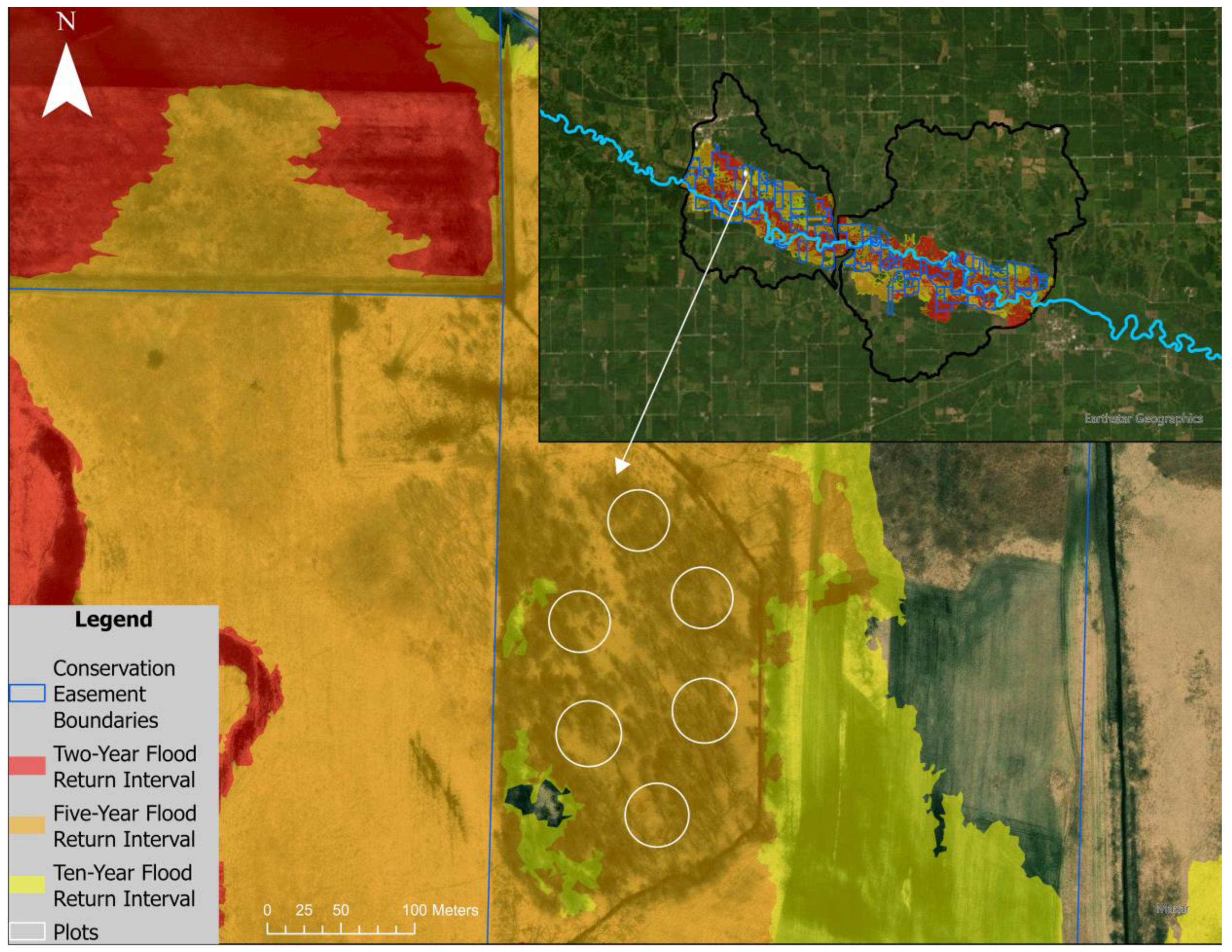
2.2. Site Selection and Survey Plot Distribution

Two HUC-12s (HUCs 070802080903 and 070802080904) were selected for study within the Iowa River Basin (Figure 1). These specific HUC-12s were selected due to the prevalence of public land and floodplain easements, which afforded access and historical management records. The study area is located on a stretch of public land within these HUC-12s, some of which is formerly cropped conservation easements that have been managed for wildlife habitat for the last 30 years. Within each HUC, the two-, five-, and ten-year FRIs were identified using flood frequency GIS data from the Iowa Department of Natural Resources [35]. These data were generated using a combination of Light Detection and Ranging (LiDAR) data and drainage-area-based regressions, which were then incorporated into one-dimensional hydraulic models using HEC-RAS [38]. Forested areas within the two-, five-, and ten-year FRIs were then identified, with preference given to areas within an easement and/or public land. Candidate areas were delineated by stand type. Forested areas that were blocked by roads, levees, or other obstructions were excluded. We then distributed 30 plots among the two-, five-, and ten-year FRIs (as seen in Figure 3) in forested areas. In total, there were 5 “sites”. Each site was a combination of a forest type and a flood return interval and contained six 20 m radius plots, a number that allowed us to collect an adequate amount of data within personnel constraints. These plots were distributed by stand type.

2.3. Forest Survey

2.3.1. Forest Survey Plot Layout

Forest survey plots were 20 m in radius, with four forest regeneration subplots 10 m from each plot center (Figure 4). Each subplot was 1.6 m in radius. Understory regeneration surveys occurred in the center of these subplots.

2.3.2. Forest Herbaceous Layer Survey

Vegetation surveys were conducted in August and September of 2022 and May and June of 2023. Within each of the 30 plots, herbaceous vegetation was assessed using one- by one-meter quadrats 10 m from the center in each of the cardinal directions (Figure 3). The vegetation was assessed using a modified version of the structural guilds listed in Diehl et al. (2019) [20]. The chosen guilds represent forbs and grass, which are the most abundant categories of vegetation on the floodplain, as well as three categories of height which are the most commonly seen in the study area (Table 1).
During late summer, vegetation stiffness was assessed using the board drop method of Kouwen (1988) [39]. In each plot, a 0.6 m by 1.8 m by 0.95 cm plywood board was dropped onto the ground. The height from the ground that it was held up by the vegetation was then measured as a proxy for vegetation stiffness.

2.3.3. Forest Overstory and Woody Regeneration Survey

Forest inventory was conducted in all plots. Each tree that was at least 5 inches (12.7 cm) in diameter at breast height (DBH) was measured for diameter and height [40]. In each of the four 1.6 m radius subplots, seedlings (defined as <2.54 cm DBH) were counted, and saplings (≥2.54 cm DBH) were measured for diameter and height. These results were summed for each plot and then expanded to a per-hectare scale.

2.3.4. Coarse Downed Wood

Coarse downed wood inventory was also taken along three transects in each plot running north, southeast, and southwest (Figure 3). Each log that was at least 7.6 cm wide and 0.9 m long was measured for center width and length [41,42]. The volume of each log was calculated by using the volume formula for cylindrical shapes:
v = πr2l
where v = volume, r = radius, and l = length. These volumes were then summed for each plot and extrapolated to determine the volume of wood per hectare.

2.4. Sediment Deposition

Historic sediment deposition was quantified using a modified version of the tree-coring analysis method of Sigafoos (1964) [43]. In our version of this method, three trees from each plot were randomly selected for coring. Based on the available length of the tree corer, the trees selected for coring were all less than 60 cm in diameter, thus limiting the mean age of cored trees to 23 years old. After coring the trees to determine their ages, we then measured the depth of sediment deposited over the root flare 50 cm from where the root went into the ground. This prevented differences in above-ground root morphology in various species from affecting the data. The amount of sediment deposited was then divided by the age to determine the rate of sediment deposition per year.

2.5. Sediment Characterization and Analyses

To determine total phosphorus content, two 10 cm deep soil samples were collected from each plot 10 m from the center in the east and west directions. Total phosphorus content (milligrams per kilogram) was extracted using nitric acid digestion. A bulk density analysis was also performed in order to calculate total phosphorus per meter squared at a depth of 10 cm. This was achieved by extracting intact 10 cm deep cores of soil using metal cylinders of a known volume, which were then dried at 105 degrees Celsius in an oven at 24 h intervals until their weights stabilized, indicating all soil moisture had been removed. Soil mass was then divided by cylinder volume to determine the bulk density. Sediment deposition rates (in centimeters per year) were multiplied by the bulk density to determine the mass of sediment deposition per year in each plot. Total phosphorus measurements were averaged per plot and then were multiplied by the deposition (in kilograms) and divided by the plot area to obtain the number of grams of deposited phosphorus per square meter.

2.6. Spatial Analyses

Forest area in the study HUC-12s was calculated by determining the area of forest in satellite imagery on ArcGIS Pro. Because almost all the forest area was within half a kilometer of the channel, we used averaged deposition rate, bulk density, and total phosphorus data from plots within half a kilometer to extrapolate data to the rest of the forest in the HUC-12s. This was achieved by multiplying the averaged yearly deposition depth by the forested area to determine the overall deposition volume, multiplying the volume by the mean bulk density to determine the deposited soil mass, and then finally multiplying the mean total P concentration by the deposited mass to determine the amount of total P deposited in the forest per year. Deposition calculations by FRIs were achieved in the same manner, with means from plots within the FRI combined with the total FRI area used to extrapolate deposition and total phosphorus data.

2.7. Statistical Analysis

Pearson correlation tests at the 0.05 level were performed in RStudio to determine relationships between deposition and vegetation parameters [44]. These tests were performed for all plots together, as well as subsets of plots grouped by closest distance from the channel, which was calculated using ArcGIS Pro. Due to the lack of normality in sampling distributions, Kruskal–Wallis ranked ANOVA testing at the 0.05 level was used to determine whether there were significant differences in deposition between the two-, five-, and ten-year FRIs. Means were taken in order to calculate overall deposition and total phosphorus in each of the flood return intervals.

3. Results

3.1. Vegetation Survey

3.1.1. Forest Overstory and Coarse Downed Wood

The forest inventory results (Figure 5) indicate a wide range of variability in the basal areas (in square meters), with the highest mean basal area per hectare overall being found in the two-year (26 square meters) as compared to the five- and ten-year FRIs, which had mean basal areas per hectare of 21 and 11 square meters, respectively. The 10-year FRI site had the most trees per hectare and the lowest variability, while the two-year and five-year FRIs had higher levels of variability with lower means (207 versus 162 and 176 trees per hectare, respectively). Regeneration was highest in the 10-year FRI, which had a mean seedling and sapling count of 1134 per hectare, and lowest in the two-year, which had a mean seedling count of just 172 per hectare. Coarse downed wood was greatest in the two-year FRI and lowest in the 10-year FRI, where there were no downed logs due to the young age of the stand. The even age distribution of the 10-year FRI meant that there was little variability compared to the two- and five-year FRIs. The distribution of the two- and five-year basal areas was similar, with no significant difference being found between the two (p = 0.26).
Species composition varied greatly between the FRIs (Figure 6). The two-year FRI comprised over 80 percent silver maple (Acer saccharinum), with the rest of the stems comprising just five other species: American elm (Ulmus americana), slippery elm (Ulmus rubra), hackberry (Celtis occidentalis), cottonwood (Populus deltoides), and green ash (Fraxinus pennsylvanica). The five-year FRI was the most diverse, with nine species present, including the aforementioned plus honeylocust (Gleditisia triacanthos), bur oak (Quercus macrocarpa), and pin oak (Quercus palustris). The 10-year FRI site comprised almost 90 percent pin oak and bur oak, with trace numbers of cottonwood, green ash, and honeylocust stems interspersed.

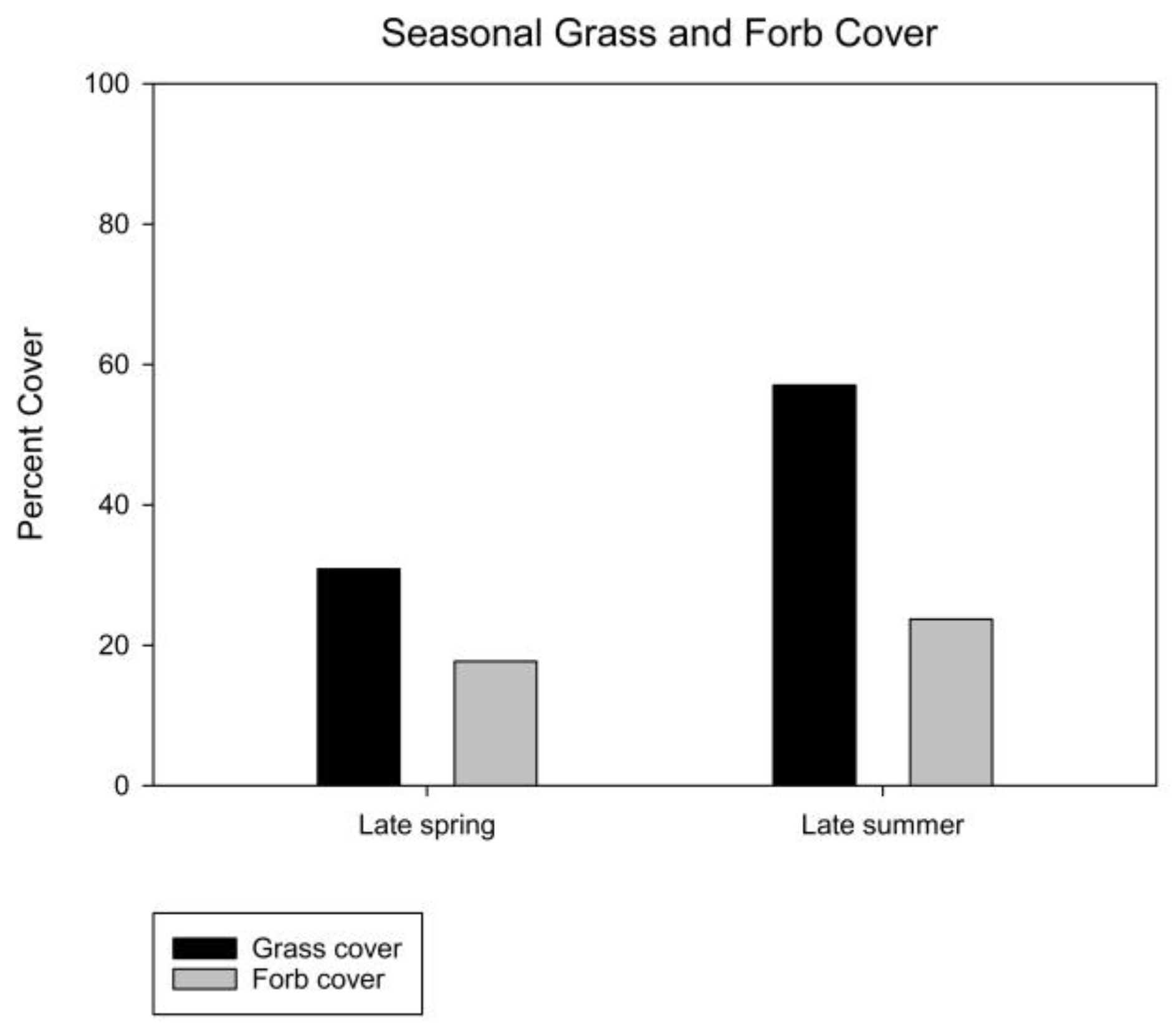
3.1.2. Forest Herbaceous Layer

Seasonal vegetation cover across all sites increased from late spring to late summer, with forb cover increasing by 34 percent and grass cover increasing by 87 percent (Figure 7). In both seasons, grass percentages exceeded forb percentages; in late spring, there was, on average, 31 percent grass cover compared to 18 percent forb cover, and in late summer, those numbers increased to 57 and 24 percent, respectively.

3.2. Correlations between Vegetation Metrics and Annual Deposition

No significant relationships were found between deposition and trees per hectare, basal area per hectare, and large woody debris. Positive correlations were found between deposition and total spring ground vegetation cover, spring tall grass cover, and all categories of spring forb cover (Table 2). The strongest correlation of these was the medium forb cover, with a correlation coefficient of 0.59 and a p-value of less than 0.001. These correlations differed from that of the late summer ground vegetation categories. For late summer, significant correlations were limited to short and medium vegetation categories, with the strongest correlation being the short forb cover parameter, which had a correlation coefficient of 0.44 and a p-value of less than 0.001. The medium forb parameter, while significant, had a much smaller correlation coefficient than late spring (r = 0.27 vs. 0.59) and a larger p-value (p = 0.008 vs. <0.001). In addition to this, vegetation stiffness was found to weakly yet significantly correlate with deposition, with a p-value of 0.036 and a correlation coefficient of 0.22.
The relationships between deposition per year and summed grass and forb categories (Figure 8) were weak overall, with correlation coefficients not exceeding 0.58. In late spring, both categories of vegetation significantly correlated with annual deposition, with the most significant and strongest Pearson correlation between the two being the forb category (p < 0.001, r = 0.58) and the weakest correlation being the grass category (p = 0.03, r = 0.22). This is despite the fact that mean forb cover is around 42 percent lower than that of grass in late spring and 58 percent lower than that of grass in late summer (Figure 7). In late summer, only the forb category was significant, but its correlation coefficient was lower than in late spring (0.33 vs. 0.58), and its p-value was higher (0.001 vs. 9.92 × 10⁻¹⁰). This contrasts with the expanded results in Table 2, which show that short grass positively correlates with deposition in late summer.

3.3. Correlations between Vegetation Characteristics and Total Phosphorus

Significant Pearson correlations between vegetation characteristics and soil phosphorus content (Table 3) were far less numerous than the soil deposition correlations. Traits that were found to correlate with soil P concentration did not always correlate with soil P mass, such as seedling and sapling count and summed grass cover. As with the deposition correlations, coefficients were weak overall, with the strongest being the late spring summed grass cover correlation (r = 0.38, p = 0.003). Both P mass and concentration significantly correlated with trees per hectare and had similar coefficients. Total spring vegetation cover also yielded similar correlations with P concentration and mass, with coefficients of 0.29 and 0.33 and p-values of 0.03 and 0.01, respectively. No parameters from the late summer category were significant, which contrasts with the results from the sediment deposition correlations.

3.4. Influence of Spatial Characteristics on Deposition

While all three FRIs had a similar distribution of deposition rates (Figure 9), the two-year FRI had a higher sample variance compared to the five- and ten-year FRIs (0.179 vs. 0.104 and 0.058, respectively). A Kruskal–Wallis ranked Analysis of Variance (ANOVA) test concluded there was no statistically significant difference (p = 0.65) between the deposition rates in the three FRIs. Pearson correlation testing between the closest distance to the channel from a given plot and the respective deposition per year revealed a weak yet significant negative correlation, with a correlation coefficient of −0.29 and a p-value of <0.001 (Figure 6). Additionally, distance from the channel negatively correlated with total phosphorus concentration (p < 0.001, r = −0.69) and total phosphorus mass (p < 0.001, r = −0.63). This is supported by the fact that clay particle percentage, which correlated significantly with total phosphorus soil content (p < 0.001, r = 0.47), was found to also negatively correlate with distance from the channel (p < 0.001, r = −0.46). The one-way ANOVAs returned no significant difference between flood return intervals either in concentration or mass.

3.5. Floodplain Sediment and Total Phosphorus Storage

Though there were no significant differences in sediment and phosphorus deposition between the three FRIs, there was a clear stratification of means in terms of phosphorus concentration, with the highest mean concentration being in the two-year FRI and the lowest in the ten-year FRI (Table 4). This is not reflected in the phosphorus mass results, which indicate that the highest phosphorus content is in the two-year FRI and the lowest is in the five. In comparison to the five-year FRI, there is 21.9 percent more deposition in the ten-year FRI. This could potentially be attributed to differences in mean density between the soils of the FRIs. The bulk density analysis revealed that the soil bulk density of the ten-year FRI was 19 percent higher than that of the two-year FRI and 26 percent higher than the five-year FRI.
Total sediment accumulation showed similar patterns to that of the phosphorus accumulation, with the highest annual deposition occurring in the two-year FRI and the lowest in the five-year FRI.
Across the entire forested floodplain within the two-, five-, and ten-year FRIs, a mean of 3.24 kg per square meter of sediment is deposited each year (Table 5). Around 37 percent of this deposited soil is comprised of clay-sized particles, which carry with them attached phosphorus. Total phosphorus deposition per square meter is 2.79 g on average.
In total, 73,691 Mg of sediment and 70.05 Mg of phosphorus are deposited in the forested areas of the two study HUC-12s every year. This represents 4 to 50 percent (median = 15.5%) of the annual sediment load that passes through the Iowa River near the study area, based on previous literature [36].

4. Discussion

4.1. Vegetation Influences on Sediment and TP

Our forest inventory correlation results contrast with those of Nanson and Beach (1977), who found that younger, denser forest stands accreted more sediment [45]. However, this difference in results could possibly be attributed to the fact the forests in our study were much less dense; therefore, it is possible that a certain level of forest density must be reached before effects on sedimentation occur. Conversely, our forest correlation results are in line with that of Rybicki et al. (2015), who found that sediment trapping increased where there were higher levels of herbaceous plants and lower amounts of trees [46]. The lack of trend with stems per hectare in our results could possibly be due to forest density patterns being irregular across many of the sites. Hence, more plots in each site could provide more clarity on this matter. Understory correlations, however, were in line with our expectations, with both cover and rigidity positively correlating with deposition. The fact that the cover of forbs, which are typically more structurally diverse than grass, repeatedly correlated strongly with deposition reflects the results of Kretz et al. (2021), who found that structural diversity positively correlated with sediment accretion [24].
The results from the soil phosphorus concentrations/mass correlations were in line with findings from a 2020 literature review, which found that grassy vegetation is the most effective at trapping particulate phosphorus [47]. The contrast in correlations between sediment deposition and phosphorus mass/concentration may be indicative of certain vegetation types being more adept at trapping particle sizes that phosphorus adsorbs to rather than sediment as a whole. Phosphorus concentrations could also be affected by local processes such as vegetative uptake and decomposition. Most of the vegetation correlations were relatively weak, however, with none of them exceeding an r value of 0.61. This indicates that other factors, such as flow paths, may influence sediment and attached phosphorus deposition, and underscores the significance of floodplains as heterogeneous landscapes with multiple interacting features and mechanisms that drive fluvial processes.
The seasonal differences in correlations could possibly be attributed to potential differences in seasonal flooding depths; in order to confirm this, further investigation is required. Further investigation could also provide more clarity regarding vegetation correlations at different distances from the channel. Although there were clear differences in vegetation correlations at different distances in this study, the plots were distributed by FRIs instead of distance. Thus, in terms of distance from the channel, there were clumps of data with large spatial gaps in between. Distributing plots evenly along a transect from the channel would provide a better understanding of the relationship between distance and vegetation correlations.

4.2. Spatial Influences on Sediment and TP

The flood return interval results contrasted with our hypothesis. The reality that the flood return interval had no bearing on sediment deposition in this study goes against all expectations at first glance, as one would expect that an area that floods more frequently should have more deposition. However, results from Moustakidis et al. (2019) show that areas that flood more frequently may also scour during floods, leading to erosion instead of deposition [18]. This could possibly explain why there is not a significant increase in sediment and total phosphorus deposition in the two-year-flood return interval.
Distance from the channel correlations were in line with other results from the literature [9,18,48,49]. The negative correlation between sedimentation and distance from the channel may reflect the deposition of coarser material, which is typically the first to deposit during a flood [50]. The significant correlations between distance from the channel and deposition, combined with the lack of differences between FRIs, indicate that distance over the floodplain is a more effective predictor of deposition rates than the spatial distribution of FRIs.

4.3. Floodplain Sediment and Total Phosphorus Storage

The sediment accretion results contrasted with our expectations, with similar deposition per square meter results being found in both the two-year and the ten-year FRIs. This could potentially be explained by past land use on the ten-year site, which was previously farmed and thus had highly compacted soil. This compaction could have had an impact on bulk density measurements, which in turn could have impacted the sediment and total phosphorus accumulation calculations. In terms of the percent of the river sediment load that was captured by the site, the results align with some of the literature but contrast with others. For example, the results align with Omengo et al. (2016), who found that 15 to 30 percent of river loads were captured by an adjacent floodplain [9], but contrast with Noe and Hupp (2009), who found that naturally vegetated floodplains store 119% of river sediment loads [14]. However, the study sites and contributing watersheds in these studies were different in terms of size and composition. Our total phosphorus accumulation results were just slightly higher than those found across the literature in a review by Gordon et al. (2020) (27.9 kg-P ha−1 year−1 vs. 21 9 kg-P ha−1 year−1) [47]. The amount of total phosphorus, however, was relatively low compared to the annual load of phosphorus in the Iowa River. This largely reflects that the total phosphorus content from the Iowa River included dissolved reactive phosphorus content, which cannot be deposited onto floodplains. Also, due to the fact that during the time of study, the state of Iowa was in a drought, the Iowa River had not flooded in over three years. Therefore, any accumulated phosphorus from previous floods could have been reduced by plant uptake and assimilation.

4.4. Study Limitations

There were a few key limitations that put constraints on this study. Firstly, the one-dimensional modeling that was used to determine the spatial extent of the FRIs was not enforced for obstructions. Thus, it is possible that the true extent of the FRIs, especially ones far from the channel, are inaccurate. Secondly, the sediment accumulation calculations in the study assume an even laminar flow pattern, which is unlikely to reflect reality. In order to determine the actual flow patterns that occur during flood events, one would need to model the flows using 2-D hydraulic modeling. Due to time constraints, modeling was not possible during this study, but it could prove useful in future investigations of the matter. Additionally, the tree-coring method for assessing sediment deposition assumes that the rate of deposition is uniform for each year, which is unlikely to be true, given the differences in flood magnitudes over time.
The correlation results connecting historic deposition to vegetation metrics reflect only the current vegetation composition; therefore, past vegetation composition and its influences could not be taken into account. In future investigations, past vegetation composition could be estimated in part by available LiDAR data. Additionally, deposition from flooding onto feldspar pads, artificial turf, or other collection mediums in future studies could provide important insights into sedimentation rates during individual flood events. This, coupled with sediment load data, could shed light on how much sediment in proportion to the sediment load is deposited during an individual flood.
Finally, some of the sites were located on conservation easements that were previously farmed. Because modern farming practices compact the soil, this could have impacted our bulk density measurements and thus impacted our calculations of total sediment and phosphorus deposition.

4.5. Floodplain Forest Influences on Water Quality

Overall, floodplain forests have the potential to trap a small proportion of the sediment that passes through the Iowa River; however, the amount the forest traps depends on the understory composition, the distance from the channel, and other interacting geomorphological and hydrological factors. Though floodplain forests are effective at trapping overbank flow sediment and phosphorus, the fact that the majority of the floodplain forest in this study was in the two- and five-year FRIs means that erosional impacts during flood events may be counteracting trapping impacts, leading to reduced storage. Additionally, floodplain heterogeneity may mask some trends in floodplain vegetation performance in terms of deposition impacts. For example, the presence of microtopography like slumps, hummocks, and meander scars may encourage concentrated flow paths. These flow paths, as well as different combinations of vegetation and spatial dynamics, may render correlations between deposition and individual plant features such as height weaker than they would be in a controlled environment. Indeed, it is possible that other factors besides vegetation exert a bigger influence on sedimentation. Flooding dynamics may also play a role in the vegetation–deposition relationship; for example, in lower flow events, forbs and grasses may have more of an impact, while in higher flow events, trees and large woody debris may be more effective at slowing overbank flow velocities and promoting deposition. Therefore, it may be that diversity in forest structure, both in terms of the overstory and understory, would be beneficial for deposition. Future studies could potentially assess the influences of forest structure diversity, as well as perhaps other influences on structure, such as the introduction of invasive plant species. These investigations could provide further insights on how to restore and manage floodplains for maximum potential deposition.

Author Contributions

Conceptualization, W.B., E.Z. and R.S.; methodology, W.B. and S.G.; formal analysis, S.G.; investigation, S.G.; data curation, S.G.; writing—original draft preparation, S.G.; writing—review and editing, W.B., E.Z. and R.S.; supervision, W.B.; project administration, W.B. and S.G.; funding acquisition, W.B. and E.Z. All authors have read and agreed to the published version of the manuscript.

Funding

This research was funded in part by the Iowa Water Center, grant number GR-024688-00007 and the Iowa Nutrient Research Center, grant number SP2022-01.

Data Availability Statement

The raw data supporting the conclusions of this article will be made available by the authors on request.

Acknowledgments

The authors would like to acknowledge support from members of the Iowa State University Streams and Buffers Lab. We especially would like to acknowledge support provided by Angel Brown, Levi Kleinmeyer, Andrew Rupiper, Kelsey Karnish, and Allyson Smithson.

Conflicts of Interest

The authors declare no conflicts of interest. The funders had no role in the design of the study; in the collection, analyses, or interpretation of data; in the writing of the manuscript; or in the decision to publish the results.

References

  1. USDA National Agricultural Statistics Service. United States Summary and State Data. 2017 Census Agric. 2017, 1, 820. [Google Scholar]
  2. Thaler, E.A.; Kwang, J.S.; Quirk, B.J.; Quarrier, C.L.; Larsen, I.J. Rates of Historical Anthropogenic Soil Erosion in the Midwestern United States. Earth’s Future 2022, 10, e2021EF002396. [Google Scholar] [CrossRef]
  3. Correll, D.L. The Role of Phosphorus in the Eutrophication of Receiving Waters: A Review. J. Environ. Qual. 1998, 27, 261–266. [Google Scholar] [CrossRef]
  4. Turner, R.E.; Rabalais, N.N.; Justic, D. Gulf of Mexico Hypoxia: Alternate States and a Legacy. Environ. Sci. Technol. 2008, 42, 2323–2327. [Google Scholar] [CrossRef] [PubMed]
  5. Mishra, R.K. The Effect of Eutrophication on Drinking Water. Br. J. Multidiscip. Adv. Stud. 2023, 4, 7–20. [Google Scholar] [CrossRef]
  6. Dodds, W.K.; Bouska, W.W.; Eitzmann, J.L.; Pilger, T.J.; Pitts, K.L.; Riley, A.J.; Schloesser, J.T.; Thornbrugh, D.J. Eutrophication of U. S. Freshwaters: Analysis of Potential Economic Damages. Environ. Sci. Technol. 2009, 43, 12–19. [Google Scholar] [CrossRef] [PubMed]
  7. Schilling, K.E.; Streeter, M.T.; Seeman, A.; Jones, C.S.; Wolter, C.F. Total Phosphorus Export from Iowa Agricultural Watersheds: Quantifying the Scope and Scale of a Regional Condition. J. Hydrol. 2020, 581, 124397. [Google Scholar] [CrossRef]
  8. Mendes, L.R.D. Edge-of-Field Technologies for Phosphorus Retention from Agricultural Drainage Discharge. Appl. Sci. 2020, 10, 634. [Google Scholar] [CrossRef]
  9. Omengo, F.O.; Alleman, T.; Geeraert, N.; Bouillon, S.; Govers, G. Sediment Deposition Patterns in a Tropical Floodplain, Tana River, Kenya. Catena 2016, 143, 57–69. [Google Scholar] [CrossRef]
  10. Wilkin, D.C.; Hebel, S.J. Erosion, Redeposition, and Delivery of Sediment to Midwestern Streams. Water Resour. Res. 1982, 18, 1278–1282. [Google Scholar] [CrossRef]
  11. Cooper, J.R.; Gilliam, J.W. Phosphorus Redistribution from Cultivated Fields into Riparian Areas. Soil Sci. Soc. Am. J. 1987, 51, 1600–1604. [Google Scholar] [CrossRef]
  12. Noe, G.B.; Hupp, C.R. Carbon, Nitrogen, and Phosphorus Accumulation in Floodplains of Atlantic Coastal Plain Rivers, USA. Ecol. Appl. 2005, 15, 1178–1190. [Google Scholar] [CrossRef]
  13. Kronvang, B.; Andersen, I.K.; Hoffmann, C.C.; Pedersen, M.L.; Ovesen, N.B.; Andersen, H.E. Water Exchange and Deposition of Sediment and Phosphorus during Inundation of Natural and Restored Lowland Floodplains. Water. Air. Soil Pollut. 2007, 181, 115–121. [Google Scholar] [CrossRef]
  14. Noe, G.B.; Hupp, C.R. Retention of Riverine Sediment and Nutrient Loads by Coastal Plain Floodplains. Ecosystems 2009, 12, 728–746. [Google Scholar] [CrossRef]
  15. Noe, G.B.; Hupp, C.R. Seasonal Variation in Nutrient Retention During Inundation of a Short-Hydroperiod Floodplain. River Res. Appl. 2007, 23, 1088–1101. [Google Scholar] [CrossRef]
  16. Kronvang, B.; Hoffmann, C.C.; Dörge, R. Sediment Deposition and Net Phosphorus Retention in a Hydraulically Restored Lowland River Floodplain in Denmark: Combining Field and Laboratory Experiments. Mar. Freshw. Res. 2009, 60, 638–646. [Google Scholar] [CrossRef]
  17. Hubbard, L.; Kolpin, D.W.; Kalkhoff, S.J.; Robertson, D.M. Nutrient and Sediment Concentrations and Corresponding Loads during the Historic June 2008 Flooding in Eastern Iowa. J. Environ. Qual. 2011, 40, 166–175. [Google Scholar] [CrossRef] [PubMed]
  18. Moustakidis, I.V.; Schilling, K.E.; Weber, L.J. Soil Total Phosphorus Deposition and Variability Patterns across the Floodplains of an Iowa River. Catena 2019, 174, 84–94. [Google Scholar] [CrossRef]
  19. Nepf, H.M.; Vivoni, E.R. Flow Structure in Depth-Limited, Vegetated Flow. J. Geophys. Res. Ocean. 2000, 105, 28547–28557. [Google Scholar] [CrossRef]
  20. Diehl, R.M.; Merritt, D.M.; Wilcox, A.C.; Scott, M.L. Applying Functional Traits to Ecogeomorphic Processes in Riparian Ecosystems. Bioscience 2017, 67, 729–743. [Google Scholar] [CrossRef]
  21. James, C.S.; Jordanova, A.A.; Nicolson, C.R. Flume Experiments and Modelling of Flow-Sediment-Vegetation Interactions. IAHS-AISH Publ. 2002, 276, 3–10. [Google Scholar]
  22. Lambrechts, T.; François, S.; Lutts, S.; Muñoz-Carpena, R.; Bielders, C.L. Impact of Plant Growth and Morphology and of Sediment Concentration on Sediment Retention Efficiency of Vegetative Filter Strips: Flume Experiments and VFSMOD Modeling. J. Hydrol. 2014, 511, 800–810. [Google Scholar] [CrossRef]
  23. Kretz, L.; Seele, C.; van der Plas, F.; Weigelt, A.; Wirth, C. Leaf Area and Pubescence Drive Sedimentation on Leaf Surfaces during Flooding. Oecologia 2020, 193, 535–545. [Google Scholar] [CrossRef] [PubMed]
  24. Kretz, L.; Koll, K.; Seele-Dilbat, C.; van der Plas, F.; Weigelt, A.; Wirth, C. Plant Structural Diversity Alters Sediment Retention on and underneath Herbaceous Vegetation in a Flume Experiment. PLoS ONE 2021, 16, e0248320. [Google Scholar] [CrossRef] [PubMed]
  25. Chen, Y.; Li, Y.; Thompson, C.; Wang, X.; Cai, T.; Chang, Y. Differential Sediment Trapping Abilities of Mangrove and Saltmarsh Vegetation in a Subtropical Estuary. Geomorphology 2018, 318, 270–282. [Google Scholar] [CrossRef]
  26. Reef, R.; Christie, E.K.; Moller, I.; Spencer, T. The Effect of Vegetation Height and Biomass on the Sediment Budget of a European Saltmarsh. Coast. Shelf Sci. 2018, 202, 125–133. [Google Scholar] [CrossRef]
  27. Boorman, L.A.; Garbutt, A.; Barratt, D. The Role of Vegetation in Determining Patterns of the Accretion of Salt Marsh Sediment. Geol. Soc. Spec. Publ. 1998, 139, 389–399. [Google Scholar] [CrossRef]
  28. Bourgoin, L.M.; Bonnet, M.P.; Martinez, J.M.; Kosuth, P.; Cochonneau, G.; Moreira-Turcq, P.; Guyot, J.L.; Vauchel, P.; Filizola, N.; Seyler, P. Temporal Dynamics of Water and Sediment Exchanges between the Curuaí Floodplain and the Amazon River, Brazil. J. Hydrol. 2007, 335, 140–156. [Google Scholar] [CrossRef]
  29. Griffith, G.E.; Omernik, J.M.; Wilton, T.F.; Pierson, S.M. Ecoregions and Subregions of Lowa: A Framework for Water Quality Assessment and Management. J. Iowa Acad. Sci. 1994, 101, 5–13. [Google Scholar]
  30. Strahler, A.N. Quantitative Analysis of Watershed Geomorphology. Eos Trans. Am. Geophys. Union 1957, 38, 913–920. [Google Scholar] [CrossRef]
  31. USGS StreamStats Program. Available online: https://www.usgs.gov/streamstats (accessed on 1 January 2024).
  32. Robertson, D.M.; Saad, D.A. SPARROW Models Used to Understand Nutrient Sources in the Mississippi/Atchafalaya River Basin. J. Environ. Qual. 2013, 42, 1422–1440. [Google Scholar] [CrossRef] [PubMed]
  33. Schilling, K.E.; Libra, R.D. Increased Baseflow in Iowa over the Second Half of the 20th Century. J. Am. Water Resour. Assoc. 2003, 39, 851–860. [Google Scholar] [CrossRef]
  34. Beck, W.J.; Moore, P.L.; Schilling, K.E.; Wolter, C.F.; Isenhart, T.M.; Cole, K.J.; Tomer, M.D. Changes in Lateral Floodplain Connectivity Accompanying Stream Channel Evolution: Implications for Sediment and Nutrient Budgets. Sci. Total Environ. 2019, 660, 1015–1028. [Google Scholar] [CrossRef] [PubMed]
  35. Iowa Department of Natural Resources Flood Gradient of the Modeled 2, 5, 10, 25, 50, 100, and 500 Year Floodplain Boundaries Download. Available online: https://geodata.iowa.gov/documents/224dab85156e420d9c3beb3188650069/about (accessed on 5 May 2023).
  36. Wu, Y.; Liu, S. Modeling of Land Use and Reservoir Effects on Nonpoint Source Pollution in a Highly Agricultural Basin. J. Environ. Monit. 2012, 14, 2350–2361. [Google Scholar] [CrossRef]
  37. USGS National Water Information System Data. Available online: https://dashboard.waterdata.usgs.gov/app/nwd/en/?aoi=default (accessed on 2 February 2024).
  38. Gilles, D.; Young, N.; Schroeder, H.; Piotrowski, J.; Chang, Y.J. Inundation Mapping Initiatives of the Iowa Flood Center: Statewide Coverage and Detailed Urban Flooding Analysis. Water 2012, 4, 85–106. [Google Scholar] [CrossRef]
  39. Kouwen, N. Field Estimation of the Biomechanical Properties of Grass. J. Hydraul. Res. 1988, 26, 559–568. [Google Scholar] [CrossRef]
  40. USDA. Forest Inventory And Analysis National Core Field Guide Volume I: Field Data Collection Procedures For Phase 2 Plots; USDA: Hutchinson, KS, USA, 2021; Volume I. [Google Scholar]
  41. Woodall, C.W.; Monleon, V.J. United States Department of Agriculture Sampling Protocol, Estimation, and Analysis Procedures for the Down Woody Materials Indicator of the FIA Program; USDA Forest Service, North Central Research Station: Asheville, NC, USA, 2005. [Google Scholar]
  42. Cordova, J.M.; Rosi-Marshall, E.L.; Yamamuro, A.M.; Lamberti, G.A. Quantity, Controls and Functions of Large Woody Debris in Midwestern USA Streams. River Res. Appl. 2007, 23, 21–33. [Google Scholar] [CrossRef]
  43. Sigafoos, R.S. Botanical Evidence of Floods and Flood-Plain Deposition; US Government Printing Office: Washington, DC, USA, 1964; Volume 485-A, p. 35. [Google Scholar]
  44. RStudio Team. RStudio: Integrated Development for R. RStudio, PBC, 2024. Available online: http://www.rstudio.com/ (accessed on 1 January 2024).
  45. Nanson, G.C.; Beach, H.F. Forest Succession and Sedimentation on a Meandering-River Floodplain, Northeast British Columbia, Canada. J. Biogeogr. 1977, 4, 229. [Google Scholar] [CrossRef]
  46. Rybicki, N.B.; Noe, G.B.; Hupp, C.; Robinson, M.E. Vegetation Composition, Nutrient, and Sediment Dynamics along a Floodplain Landscape. River Syst. 2015, 21, 109–123. [Google Scholar] [CrossRef]
  47. Gordon, B.A.; Dorothy, O.; Lenhart, C.F. Nutrient Retention in Ecologically Functional Floodplains: A Review. Water 2020, 12, 2762. [Google Scholar] [CrossRef]
  48. Asselman, N.E.M.; Middelkoop, H. Floodplain Sedimentation: Quantities, Patterns and Processes. Earth Surf. Process. Landforms 1995, 20, 481–499. [Google Scholar] [CrossRef]
  49. Walling, D.E.; Owens, P.N.; Leeks, G.J.L. The Role of Channel and Floodplain Storage in the Suspended Sediment Budget of the River Ouse, Yorkshire, UK. Geomorphology 1998, 22, 225–242. [Google Scholar] [CrossRef]
  50. Walling, D.E.; He, Q. The Spatial Variability of Overbank Sedimentation on River Floodplains. Geomorphology 1998, 24, 209–223. [Google Scholar] [CrossRef]
Figure 1. Iowa River Basin and study area. Study area consisted of the two-, five- and ten-year FRIs in the two study HUC-12s. River elevation in the study HUC-12s starts at 234 m and ends at 225 m above sea level. Floodplain elevation in the FRIs ranges from 225 to 237 m above sea level. Data from the Iowa Department of Natural Resources [35].
Hydrology 11 00057 g001
Figure 2. Number of Iowa River flood events over time near the study area. Data from the USGS National Water Dashboard [37].
Hydrology 11 00057 g002
Figure 3. Example of a site. Six 20-m radius plots were established in a forested area in the five-year FRI.
Hydrology 11 00057 g003
Figure 4. Plot diagram. Small squares represent vegetation quadrats. The circles around them represent regeneration subplots. The three lines represent the coarse downed wood transects.
Hydrology 11 00057 g004
Figure 5. Forest inventory results from the two-, five-, and 10-year FRIs. Black dots indicate outliers.
Hydrology 11 00057 g005
Figure 6. Species composition of the 2-, 5-, and 10-year FRI sites.
Hydrology 11 00057 g006
Figure 7. Mean summed cover for grass and forb categories for late spring and late summer.
Hydrology 11 00057 g007
Figure 8. Scatterplots depicting relationships between deposition and seasonal summed grass and forb cover. (ad) The relationship between deposition rate per year in centimeters and the summed height sub categories (short, medium, and tall) for either forbs or grass in their respective seasons.
Hydrology 11 00057 g008
Figure 9. Annual deposition rate in the two-, five-, and ten-year FRIs.
Hydrology 11 00057 g009
Table 1. Vegetation structural guilds.
CategoryHeight Requirement
Short grass<25 cm
Short forb
Medium grass25–50 cm
Medium forb
Tall grass>50 cm
Tall forb
Table 2. Significant Pearson correlations relating deposition and vegetation characteristics.
CategoryParameterPearson Correlation p-ValuePearson Correlation Coefficient
Late spring ground vegetation coverTotal ground vegetation cover<0.0010.42
Tall grass cover0.0110.26
Tall forb cover0.0010.32
Medium forb cover<0.0010.59
Short forb cover<0.0010.34
Late summer ground vegetation coverShort grass cover0.0380.21
Medium forb cover0.0080.27
Short forb cover<0.0010.44
Vegetation stiffnessBoard drop0.0360.22
Table 3. Significant Pearson correlations relating total phosphorus soil mass/concentration and vegetation characteristics for all sites. Correlations were considered significant at p < 0.05.
CategoryParameterCorrelation Coefficient for P Concentration *Correlation Coefficient for P Mass *
Forest inventoryBasal area per hectare-0.12
Trees per hectare0.290.31
Total seedlings and saplings−0.34-
Late spring coverTotal cover spring0.290.33
Tall grass cover-0.32
Summed grass cover0.38-
* P concentration measured in mg/kg. P mass measured in g/m3.
Table 4. Sediment and phosphorus accumulated per year in the study sites.
Two-Year FRIFive-Year FRITen-Year FRI
Mean bulk density (kg/m3) 880.3832.21049.5
Mean percent clay38.228.835.1
Annual sediment deposition per square meter (kg/m2)3.762.773.43
Mean P concentration (mg/kg)915.2841.0785.8
Annual phosphorus deposition per square meter (g/m2)3.442.332.70
Table 5. Summary of sediment and phosphorus accumulated per year in the forested areas in the study HUC-12s.
ParameterTotal
Total area (Ha)1879
Mean bulk density (kg/m3)897.19
Mean percent clay36.9
Total annual sediment deposition (Mg)73,691
Annual sediment deposition per square meter (kg/m2)3.92
Mean P concentration (mg/kg)950.64
Total annual phosphorus deposition (Mg)70.05
Annual phosphorus deposition per square meter (g/m2)3.73
Disclaimer/Publisher’s Note: The statements, opinions and data contained in all publications are solely those of the individual author(s) and contributor(s) and not of MDPI and/or the editor(s). MDPI and/or the editor(s) disclaim responsibility for any injury to people or property resulting from any ideas, methods, instructions or products referred to in the content.

