Article

Agricultural Water Footprints and Productivity in the Colorado River Basin

Department of Agricultural & Resource Economics, University of Arizona, Tucson, AZ 85721, USA
*
Author to whom correspondence should be addressed.
Hydrology 2024, 11(1), 5; https://doi.org/10.3390/hydrology11010005
Submission received: 20 November 2023 / Revised: 23 December 2023 / Accepted: 26 December 2023 / Published: 30 December 2023
(This article belongs to the Special Issue Water Resources Management under Uncertainty and Climate Change)

Abstract

:
The Colorado River provides water to 40 million people in the U.S. Southwest, with river basin spanning 250,000 square miles (647,497 km2). Quantitative water rights assigned to U.S. states, Mexico, and tribes in the Colorado Basin exceed annual streamflows. Climate change is expected to limit streamflows further. To balance water demands with supplies, unprecedented water-use cutbacks have been proposed, primarily for agriculture, which consumes more than 60% of the Basin’s water. This study develops county-level, Basin-wide measures of agricultural economic water productivity, water footprints, and irrigation cash rent premiums, to inform conservation programs and compensation schemes. These measures identify areas where conservation costs in terms of foregone crop production or farm income are high or low. Crop sales averaged USD 814 per acre foot (AF) (USD 0.66/m3) of water consumed in the Lower Basin and 131 USD/AF (USD 0.11/m3) in the Upper Basin. Crop sales minus crop-specific input costs averaged 485 USD/AF (USD 0.39/m3) in the Lower Basin and 93 USD/AF (USD 0.08 per m3) in the Upper Basin. The blue water footprint (BWF) was 1.2 AF/USD 1K (1480 m3/USD1K) of water per thousand dollars of crop sales in the Lower Basin and 7.6 AF/USD 1K (9374 m3/USD1K) in the Upper Basin. Counties with higher water consumption per acre have a lower BWF.

1. Introduction

The Colorado River Basin spans seven states in the United States, two states in Mexico, and the lands of 30 federally recognized tribes. The Colorado River provides water for the environment, agriculture, industry, and an estimated 40 million people in the Southwestern United States [1]. In the 250,000-square-mile (647,497 km2) Colorado River Basin, U.S. states, Mexico, and tribes have been assigned the right to use a volume of water that exceeds the volume of water that exists in the system. The Colorado River Compact of 1922 and the 1944 Water Treaty with Mexico allocated 7.5 million acre feet (maf) (9.25 km3) to Upper Basin States (Colorado, New Mexico, Utah, and Wyoming), 7.5 maf (9.25 km3) to Lower Basin States (Arizona, California, and Nevada), and 1.5 maf (1.85 km3) to Mexico, giving a total of 16.5 maf (20.35 km3) [2,3]. The 1922 Colorado River Compact [2] was negotiated during a time when river flows were high compared with reconstructed records [4,5]. Since 2000, river flows have averaged 12.3 maf/year (15.2 km3/year) [6,7]. Storage at the region’s two largest reservoirs, Lakes Powell and Mead (as well as other regional reservoirs) have dropped significantly [1,8]. Climate change is expected to further limit streamflows due to changes in basin-wide precipitation, snowpack, and temperatures [9,10,11,12]. Additionally, with increases in temperature, water demand for agricultural production, as well as electricity production, is expected to increase [9], placing further stress on the river’s supply.
To balance water demands with supplies, unprecedented water-use cutbacks have been proposed and implemented. In 2007, Basin States adopted the Interim Guidelines [8] to avoid water cutbacks, through the creation of “Intentionally Created Surplus” water. Through this agreement, water is made available as surplus to be stored in Lake Mead, in order to maintain reservoir levels above elevations that trigger water cutbacks. In 2014, the US Bureau of Reclamation (USBR) and Basin States agreed to initiate pilot programs to compensate water users for reducing consumptive water use, with saved water to be stored in Lakes Powell and Mead [13]. Contracting parties were overwhelmingly agricultural entities, with conservation achieved primarily through fallowing and deficit irrigation, and, to a lesser extent, improved irrigation efficiency. From 2015 to 2018, the Upper Basin Pilot Program implemented projects to conserve 47,280 acre-feet (58,318,934 m3) of water, while from 2015 to 2019, the Lower Basin Pilot Program initiated projects estimated to conserve 175,347 acre-feet (216,287,018 m3) of Colorado River water in Lake Mead by 2035 [13].
As drought has persisted, however, and demand continues to draw down reservoir levels, the 2019 Drought Contingency Plans (DCP) [14] were signed by the seven Basin States and the Bureau of Reclamation, setting out guidelines for spreading predicted shortfalls across users in the Basin and curtailing use to reduce the likelihood of further cutbacks. Since the DCP took effect, Tier Zero-, One-, and Two-level cutbacks have been declared, resulting in water supply cuts to Arizona and Nevada. The likelihood of further shortage has prompted consideration of additional measures to significantly reduce water use across the Basin prior to the 2026 expiration of the Interim Guidelines [15].
In 2022, Congress enacted the Inflation Reduction Act (IRA) (P.L. 117-169), which authorized funding for drought mitigation in western states, giving priority to areas served by the Colorado River [15]. Funds were authorized from 2023 to 2026 for, among other measures, compensation payments for entities voluntarily reducing water diversions or consumptive use. Agreements could be for a single year or multiple years. Saved water would be stored in Lakes Mead or Powell. Payment rates were 330 USD/AF (USD 0.27/m3) for one-year agreements, 365 USD/AF (USD 0.30/m3) for two-year agreements and 400 USD/AF (USD 0.32/m3) for three-year agreements. In 2023, the Bureau of Reclamation, administering the program, announced it would also consider higher “contractor proposed” payment rates, given supporting conservation and cost justifications. In addition, the Upper Basin revived its pilot program, setting a base payment rate of 150 USD/AF (USD 0.12/m3) of water conserved [16].
In May 2023, the Lower Basin States (Arizona, California, and Nevada) submitted a plan to the US Bureau of Reclamation (USBR) to conserve a total of 1.5 maf (1.85 km3) of Colorado River water by the end of 2024, with a cumulative total of 3 maf (3.70 km3) by the end of 2026 [17]. While 2.3 maf (2.84km3) of conservation was to be voluntary, with compensation coming from IRA funds, the remaining 0.7 maf (0.86 km3) would either be uncompensated or compensated by state or local entities. USBR has tentatively accepted this plan as their preferred management alternative for the Basin [1].
To balance Basin supply and demand, policy analyses suggest agriculture will significantly reduce its consumptive water use [8,18,19,20,21,22]. Agricultural water conservation and reallocation has become a policy focus for a number of reasons. First, agriculture accounts for more than 60% of consumptive water use in the Upper and Lower Basins [18,23] and 80% of total water withdrawals across the entirety of the Basin States [24]. So, compared to other sectors, smaller percentage reductions in agricultural use could allow much larger percentage increases in other uses [25,26], and could account for a larger absolute amount of regional conservation. Second, marginal values of water use in agriculture tend to be smaller than values in other sectors [27,28,29]. Third, while estimated costs of agricultural conservation range from 150 to 750 USD/AF/year (USD 0.12–USD 0.61/m3/year) [18], costs for other options are considerably larger. These include importation from other regions (700–3499 USD/AF/year) (0.57–2.84 USD/m3/year), desalination (750–2100 USD/AF/year) (0.61–1.70 USD/m3/year), and municipal-, industrial-, and gray-water reuse (1500–4200 USD/AF/year) (1.22–3.41 USD/m3/year) [18]. Fourth, while agricultural conservation could be feasibly implemented in the near term, other infrastructure options may not be feasible for 15 to 30 years [18].
This study develops agricultural water productivity measures for counties in Upper and Lower Colorado River Basin States, to inform policy decisions. These productivity measures include economic water productivity (on both a gross-value and net-value basis), blue water footprints of crop production, and rental rate premiums for irrigated cropland. The reported measures rely on county-level agricultural water consumptive use data from a national survey, matched to corresponding county-level economic data. We assess the variation in water productivity metrics across the Colorado River Basin, how well they are correlated with each other, and how well they are correlated with water use intensity (water consumed per unit of irrigated land area).
Results provide estimates of the opportunity cost of reallocating water away from agriculture in terms of reductions in the value of regional crop production and farm income. The current policy emphasis for water conservation in the Colorado Basin emphasizes compensated, voluntary reductions in agricultural consumptive water use. Results identify areas where current compensation payment rates are more or less likely to be attractive to crop producers. They also serve to develop estimates of total payments needed to conserve different quantities of water.

2. Materials and Methods

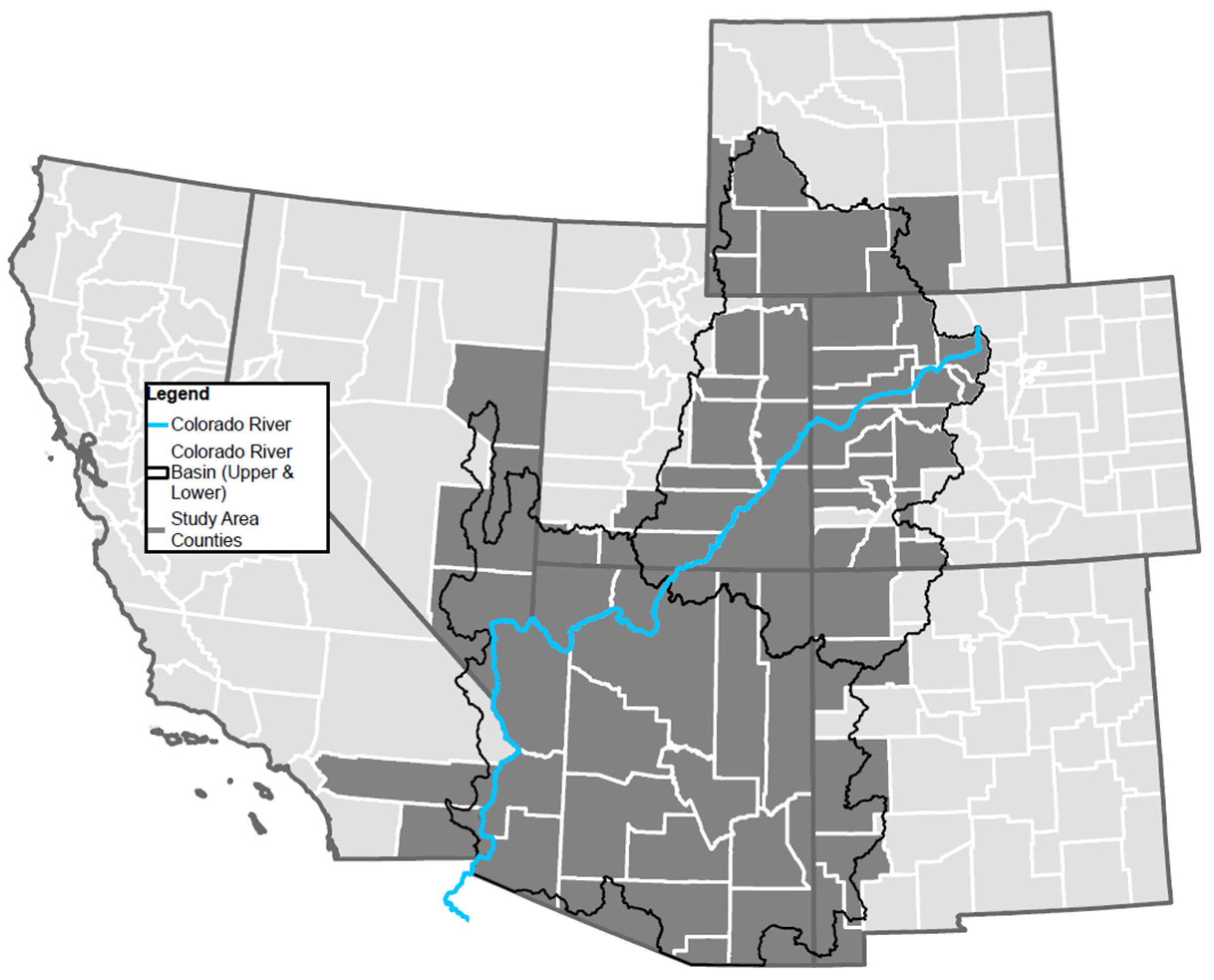
2.1. The Colorado Basin Study Area

The study area includes counties in seven Colorado Basin States (Figure 1). Water productivity measures for this study are reported as county-level averages. Five counties from Wyoming were included in this analysis. Sublette and Sweetwater counties lie predominantly within the Colorado River Basin, while Lincoln and Uintah counties have irrigated land within the Bear River Basin, as well as the Colorado River Basin [30]. While Carbon County lies predominantly outside of the Colorado River Basin, it does contain irrigated acres within it. Past economic assessments of water cutbacks in the Wyoming portion of the Colorado River Basin have included Carbon County [31].
We included 18 Colorado counties: Archuleta, Delta, Eagle, Garfield, Grand, Gunnison, Hinsdale, La Plata, Mesa, Moffat, Montezuma, Montrose, Ouray, Pitkin, Rio Blanco, Routt, San Miguel, and Summit. Saguache County was not included, as more than 90% of its irrigated acreage has been estimated to be in the Rio Grande Basin [30]. Dolores County was excluded because acreage there is dominated by dryland farming, which historically has accounted for more than 75% of cropland acres [32]. Data were not available to distinguish between irrigated and non-irrigated output. San Juan County was also excluded, because neither the US Department of Agriculture (USDA) nor the US Geological Survey (USGS) report data on irrigated acreage or water use for that county.
For New Mexico, San Juan County, which lies in the Upper Basin, was included, as were Catron, Grant, Hidalgo, and McKinley counties, lying solely or predominantly in the Lower Basin. Cibola County was excluded, as its acres lie predominantly outside the Basin. Following [30], all counties in Arizona were included in the Basin-wide analysis, as were Clark, Lincoln, and White Pine counties in Nevada, Imperial and Riverside counties in California and Carbon, Daggett, Duchesne, Emery, Garfield, Grand, Kane, San Juan, Uintah, Washington, and Wayne counties in Utah.

2.2. Water Productivity and Footprint Measures

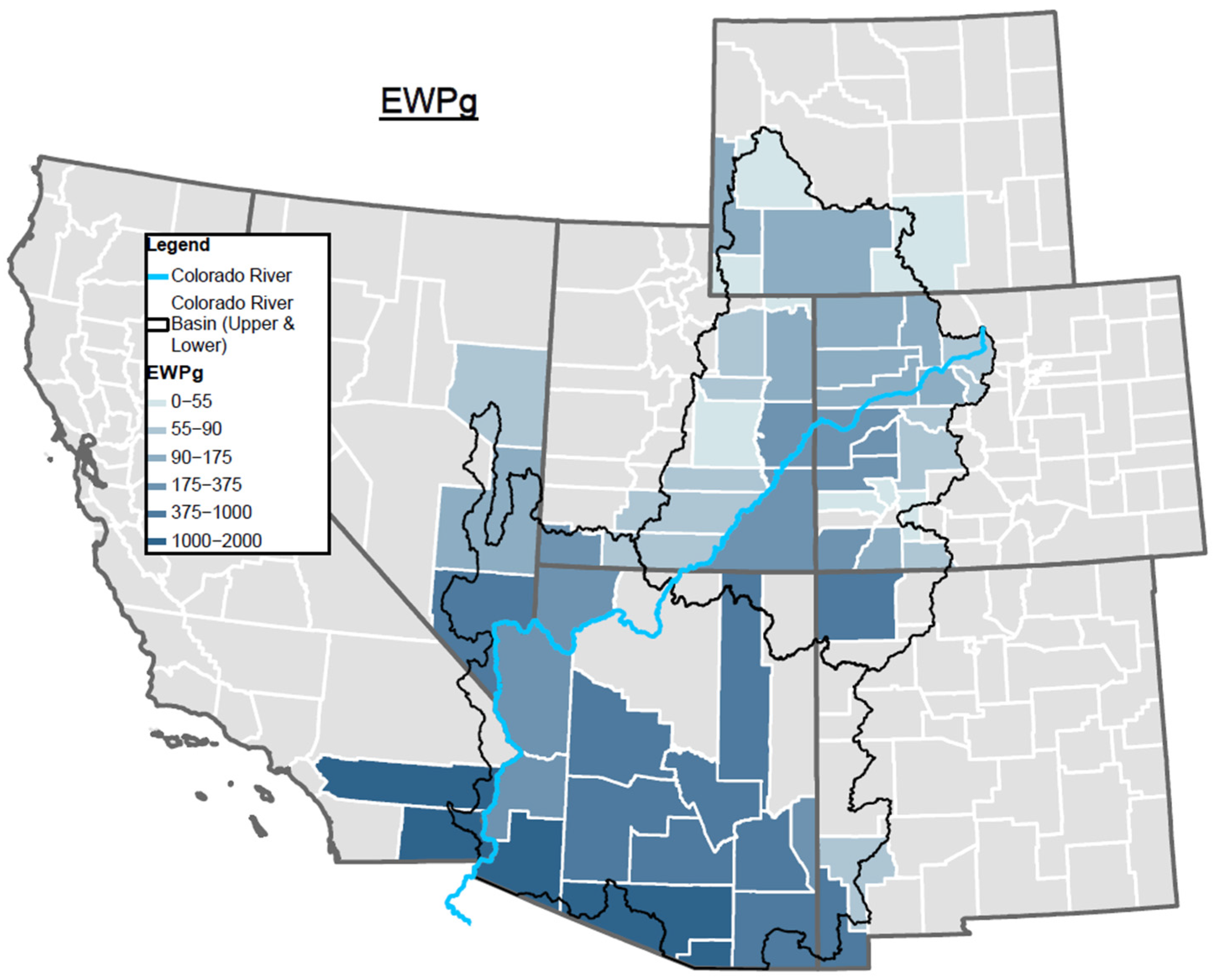
2.2.1. Economic Water Productivity: Gross Return Basis (EWPg)

Water productivity measures outputs generated per unit of water used. Productivity can be measured in terms of physical output (e.g., kg of crop produced) per unit of water consumed. Economic water productivity, in contrast, measures outputs in terms of a common monetary unit. This is often revenue generated (output times price). Economic water productivity allows one to compare crop outputs using a common value (as opposed to comparing MT or kg for multiple different crops). It also approximates gross economic benefits per unit of water consumed.
Economic water productivity (EWPg) of Colorado River Basin counties is computed using the dollar value of crop marketings (gross returns, denoted by the ‘g’ subscript) in 2015 in each county, divided by the consumptive use of water for irrigation in each county
EWPg = CM/W
where CM = county crop marketings in USD and W = county consumptive use of water for irrigation in acre-feet.
County-level data for crop revenues for 2015 were obtained from the US Department of Commerce, Bureau of Economic Analysis Regional Economic Accounts, which reports these data annually [33]. The year 2015 is used because the USGS reports data for consumptive use of water for irrigation from its 2015 national survey [24]. The USGS reports on county-level water withdrawals every five years. Reports of consumptive use were discontinued after the 1995 survey, but were resumed for the 2015 survey. The most recent USGS survey data available are from 2015 [34].
The USGS [24] defines the consumptive use of irrigation water as “the fraction of water that was originally withdrawn from a source for irrigation and is subsequently removed from availability owing to evaporation, transpiration, or incorporation into crops (p. 30)”. For most states, USGS relies on various sources to base consumptive-use estimates on coefficients, irrigation-system efficiencies, or theoretical crop requirements. Additionally, the USGS National Water Use Science Project (NWUSP) developed evapotranspiration estimates based on 1 km-scale MODIS satellite data which, in turn, are analyzed through the Operational Simplified Surface Energy Balance (SSEBop) model [35], to interpret consumptive-water-use estimates on irrigated lands. Consumptive-use estimates in California, Colorado, and Wyoming were based primarily on SSEBop model data.
For a few counties with very small irrigated acreage, computed EWPg measures were implausibly large. Inspection of data for these anomalous counties suggests this is because the USGS data undercount water use (the denominator in the EWPg equation). For these counties, estimates of irrigated acreage were an order of magnitude lower than reported irrigated acreage from other sources such as the USDA National Agricultural Statistical Service (NASS), NASS field offices in Basin States, or state offices of the engineer. In one other case, Catron County, New Mexico, estimated water consumption per acre was double that of all surrounding counties with similar crop mixes. These anomalous counties were excluded from our reported EWPg calculations. Their exclusion has few implications for Basin-wide water use or productivity as combined they accounted for less than 0.16% of Basin irrigation consumptive use and less than 0.3% of crop sales.
The BEA data used for the EWPg numerator are crop cash receipts. Cash receipts, however, exclude the cash value of feed crops used directly on farm and which are not marketed. In locations where such non-marketed production is significant, failure to account for this could also understate EWPg significantly. State-level data from USDA for the total value of hay produced (including hay consumed directly, and not sold) suggest non-marketed values are significant in Basin States. If one compares state-level USDA data with state-level BEA data for cash receipts, the total value of hay production exceeds the value of hay cash receipts by 24% in California, 66% in Nevada, roughly 80% in Utah and Wyoming, and roughly 90% in Arizona, Colorado, and New Mexico.
One can adjust EWPg upward to account for this additional value of non-marketed hay, which we denote as EWPh. EWPh is calculated by applying a percentage upward adjustment to EWPg equal to the percent-value by which total hay production exceeds hay sales, multiplied by hay sales as a percentage of total crop sales. The upward adjustment in EWPg will be larger in counties where non-marketed hay sales are a larger share of hay production and where hay production is a larger share of total crop sales. Unfortunately, county-level data on non-marketed hay sales are not available. To calculate EWPh at the county level, we assumed county-level shares of non-marketed production equaled the statewide average. County-level estimates of hay sales as a share of total crop sales (the other part of the adjustment factor) were obtained from county-level data from the 2012 and 2017 Censuses of Agriculture. Average values across the two years were applied to develop county-level measures of EWPh.

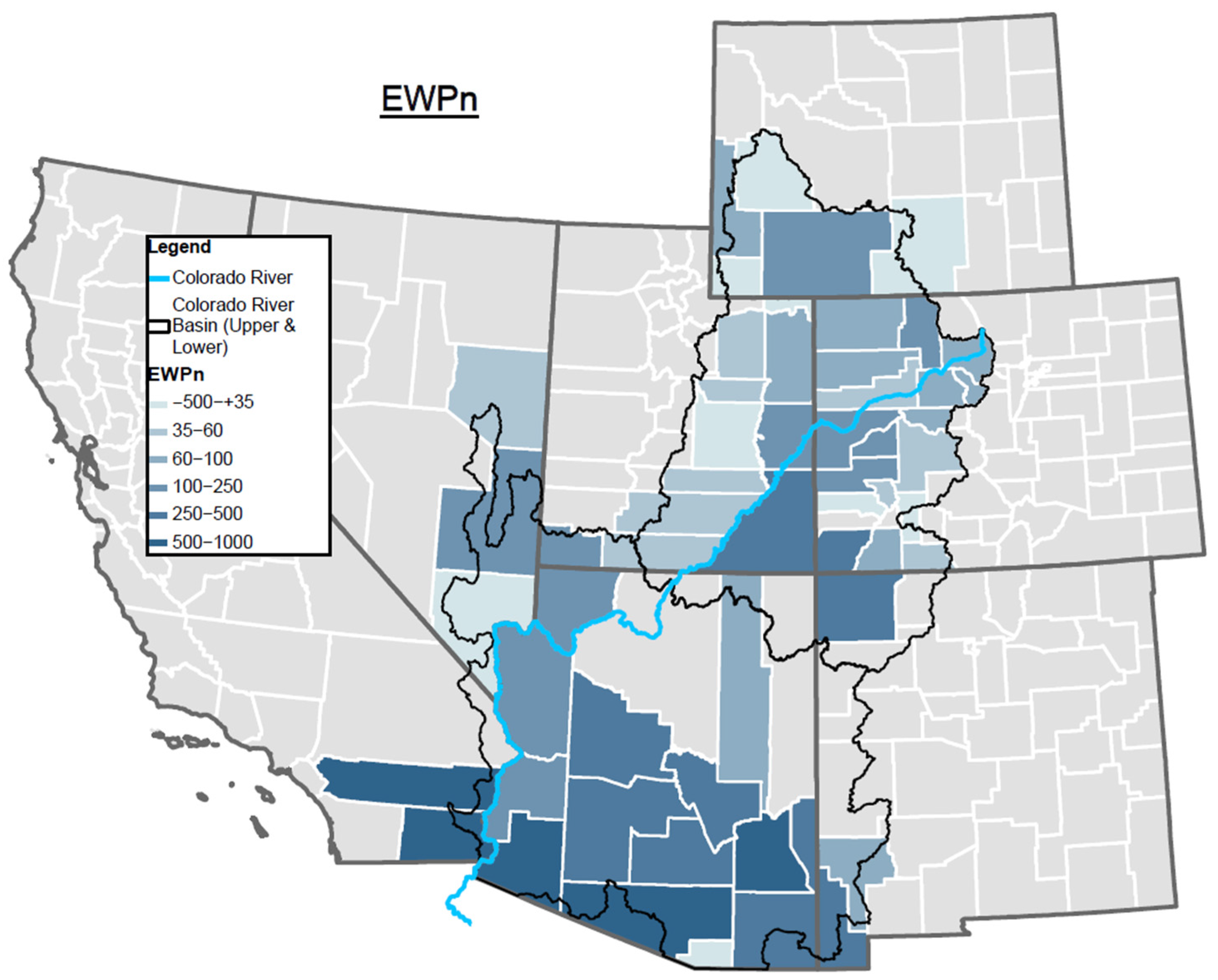
2.2.2. Economic Water Productivity: Net Return Basis (EWPn)

Some have argued that EWP based on net economic returns is a preferable metric to EWP based on gross returns [36]. Measuring effects on net returns is also more in keeping with principles of cost–benefit analysis required of U.S. federal water projects. Costs of production data needed for such calculations, however, are often unavailable, so that applied analyses rely on an EWP based on gross returns [36]. While data are not available to net out all production costs from our county-level data, it is possible to deduct some costs.
The BEA farm income-and-expense data series report costs for three types of inputs: those that are specific to crop production (seed, fertilizers, and agricultural chemicals), those specific to livestock production (animal feed, and replacement animals), and those that may be applied to either crops or livestock (labor, energy, and other services).
This study constructed an economic water productivity measure, EWPn, measuring net returns per acre of water consumed as
EWPn = (CM − S − F − AgC − L)/W
where CM = county crop marketings in U.S. dollars (USD), S = cost of seed in USD, F = cost of fertilizers in USD, AgC = cost of agricultural chemicals in USD, L = cost of crop-specific labor USD, and W = county consumptive use of water used for irrigation in acre-feet.
Data for costs of seed, fertilizers and agricultural chemicals all come from [33]. BEA data do not report crop-specific labor costs. However, the US Department of Labor’s Quarterly Census of Employment and Wages (QCEW) report county-level wage payments for workers engaged in crop production and in support activities for crop production [37]. This latter category includes workers employed by farm-labor contractors, as well as workers providing crop-specific custom services.
The QCEW reports wages for industries that are covered by state unemployment insurance (UI). However, those working on farms or for farm-labor contractors are not covered by state UI programs in many states. While farm employees have mandatory UI coverage or almost complete voluntary coverage in Arizona and California, this is not the case in the other Basin States [38]. Agricultural labor costs (L) are likely undercounted and EWPn overcounted in many counties in the other Basin States.
The numerator of EWPn nets out costs of inputs that are solely crop-specific. Yet it does not net out fuel, machinery, and capital costs that are associated with crop production. As such, EWPn overstates somewhat the net returns per unit of water consumed.

2.2.3. Blue Water Footprint (BWF)

A blue water footprint (BWF) is “the volume of surface and ground water consumed (evaporated) as a result of the production of a good” (p.1578) [39]. The BWF refers to water consumed via purposeful irrigation. This is distinct from the green water footprint, which refers to rainwater consumed by crops. For individual crops, BWF can be measured on a per-year, per-metric ton or per-kilocalorie (energy) basis [40,41]. At a more aggregate, sectoral level of analysis, the output measure is often expressed in terms of monetary units, such as the gross value of output [41,42], or value added [43].
The sectoral blue water footprint (BWF) of crop production in each county can be expressed as the simple reciprocal of the economic water productivity measure EWPg.
BWF = 1/EWPg = W/CM
where CM = county crop marketings in USD and W = county consumptive use of water used in irrigation in acre-feet. As with the EWPg, counties with implausible, anomalous values contradicted by other secondary data, were excluded.

2.2.4. Cash Rent Premiums for Irrigated Land

Another method used to estimate the value of water for irrigation is to compare cash rents for irrigated versus non-irrigated land in the same area [44,45]. Cash rents are a better metric than farm sales prices, because the latter may be affected by speculative purchase of agricultural land for conversion to commercial or residential real estate. Cash rents, in contrast, reflect current returns to farming. Some analysts further adjust the irrigated–non-irrigated differential by differences in property taxes or certain additional costs associated with irrigated agriculture [46,47]. However, in efficient land rental markets, cash rents may already reflect these additional cost differences [48].
Data on agricultural cash rental rates come from the U.S. Department of Agriculture (USDA) Cash Rents Survey. The 2008 and 2014 Farm Bills mandated that USDA collect data on mean rental rates for all U.S. counties with 20,000 acres or more of cropland and pasture. USDA did not conduct a survey for 2015. This study reports irrigation cash rent premiums for 2016 as most closely matching USGS 2015 data on irrigation consumptive use of water. Cash rents can reflect market conditions with a lag, with slow year-over-year variation [49,50,51], so irrigation conditions and practices in the previous year may be captured in cash rental rates in the following year. Whenever possible, county-level cash rental rates were used. In some cases, there were not enough responses in a county to meet USDA nondisclosure requirements. In these cases, data for the non-disclosed counties were reported at a more aggregate agricultural-district or combined-counties level. For each county, the most disaggregated data available were used.
The cash rent irrigation premium (per acre) Pa was calculated as
Pa = RCi − max [RCn, RPn]
where RCi = the cash rental rate for irrigated cropland, RCn = the cash rental rate for non- irrigated cropland, and RPn = the cash rental rate for non-irrigated pastureland.
All values are in dollars per acre. For several counties in the Colorado River Basin, non-irrigated farming is not economically viable, and non-irrigated-cropland rental markets are not active. In these areas, non-irrigated pastureland may be the only viable non-irrigated agricultural land use.

2.2.5. Cash Rent Premiums per Unit of Water

Some analysts have estimated the value of water for irrigation in terms of cash rent premiums per unit of water used for a single crop [48] or multiple, dominant crops grown in an area [52]. This measure accounts for the fact that different crops and regions have different water requirements. The present study makes use of the USGS 2015 county-level estimates of consumptive water use for irrigation. These data were used to derive county-level measures of water consumed (W) for irrigation per irrigated acre (Ai). As with the EWP measures, results were not reported for anomalous counties with data inconsistent with corroborating statistics. The cash rental premium per acre-foot of water, Pw, is given by
Pw = Pa/[W/Ai]

2.2.6. Green Water Footprint

The green water footprint (GWF) refers to the consumptive use (primarily by crops) of rain water [39,43]. The sophisticated data and modeling requirements needed to estimate GWF for the Colorado Basin are beyond the scope of this article. Other studies have developed county-level estimates of growing-season precipitation, GWF, and related measures [53,54,55]. These, however, often assume water use based on cropping systems that dominate the U.S. Midwest, which are not actually prevalent in the Colorado River Basin. In much of the world, green water is a significant source of water consumption for crop production. Not so for the Colorado Basin. Estimates for the GWF of crop production for the region range from 0 to 10 mm (0 to 0.4 inches) per year [39]. This suggests that green water could contribute only minimally to regional-crop water requirements.

3. Results

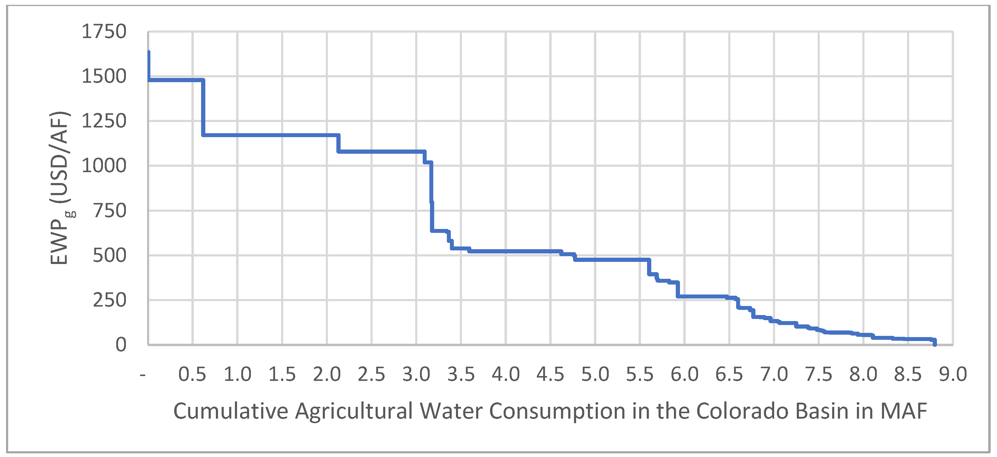
3.1. Economic Water Productivity (Gross Returns Basis)

Economic Water Productivity (EWPg) averaged across the entire Basin was 618 USD/AF (USD 0.50/m3) (Table 1). There were marked differences between the Upper and Lower Basins. EWPg averaged 814 USD/AF (USD 0.66/m3) in the Lower Basin, while it averaged 131 USD/AF (USD 0.11/m3) in the Upper Basin. The Upper Basin accounted for 29% of water consumed, but generated just 6% of crop receipts. The Lower Basin accounted for the bulk of water consumed, 71%, but generated an even larger share of production value, 94% of crop receipts. Sorting counties from highest to lowest EWPg, counties that accounted for 24% of water consumption generated 49% of all crop receipts; counties that accounted for 41% of water consumption generated 74% of sales; counties consuming two-thirds of the water accounted for 93% of sales. Conversely, counties with the lowest EWPg accounted for 25% of water consumption, but generated only 3% of Basin crop sales. Lower-EWPg counties, which accounted for a third of Basin irrigation water consumption, generated only 7% of crop sales. Mapping the distribution of EWPg, values tend to be higher in the southwest part of the Basin along the Lower Colorado River mainstem and along the U.S.—Mexico border (Figure 2). Generally, EWPg, values tend to decline moving upriver and to the northeast.
Figure 3 shows the average and marginal EWPg across the entirety of the Colorado Basin. EWPg varied widely across the Basin. Agricultural water consumption totaled 8.8 maf (10.85 km3) across the Basin. When ranked by value of EWPg, counties with the highest economic water productivity (ranging between 1000 and 1750 USD/AF (USD 0.81–USD 1.42/m3) in EWPg) consumed roughly 3 million acre-feet (maf) (3.7 km3) of irrigation water. Meanwhile, another 3 maf (3.7 km3) was consumed by counties with the lowest EWPg values, which ranged between 0 and 500 USD/AF (USD 0–USD 0.41/m3). Counties with an EWPg below 250 USD/AF (USD 0.20/m3) consumed slightly more than 2 maf (2.47 km3).
Gross returns represent an estimate of revenues generated from the sale of agricultural production. Gross returns are not representative of losses to producers from foregoing water, because they include the value of spending on inputs for production, which are avoided if cropland is fallowed. Net returns are a better measure of losses for producers. Gross returns, however, may be useful in estimating the distributional impacts of crop fallowing on the broader agricultural economy. The total compensation needed to mitigate impacts across the broader agricultural economy, including farm labor and input suppliers, is better represented by gross, rather than net returns [56].
Accounting for the value on non-marketed, directly consumed hay had little effect on the relative rankings of counties by EWPg. The Spearman rank correlation coefficient between EWPg and EWPh (which accounts for un-marketed hay values) was 0.99 (p = 0.0000005). The median (average) upward adjustment of EWPh above EWPg across counties was 48 USD/AF (USD 60/AF) (0.04/m3 to 0.05/m3). For six counties, the adjustment exceeded 100 USD/AF (USD 0.08/m3), suggesting that non-marketed feed production can be an important source of irrigation water demand.

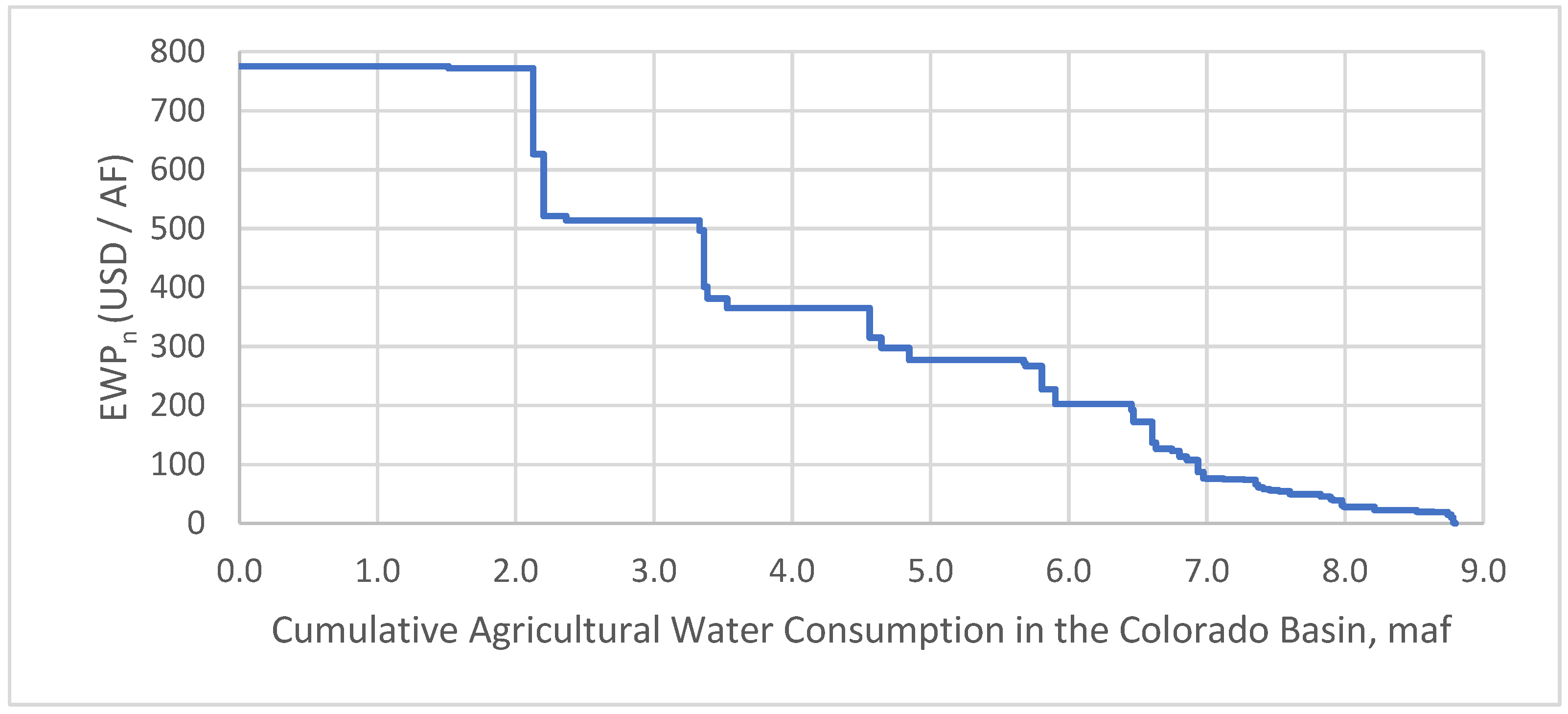
3.2. Economic Water Productivity (Net Returns Basis)

For the overall pattern of water productivity based on net returns (crop receipts minus allocable, crop-specific input costs) EWPn is similar to the EWPg. Again, EWPn values are higher for counties along the Colorado River mainstem and the US–Mexico border (Figure 4). Four counties, Imperial and Riverside in California and Yuma and Maricopa in Arizona, accounted for 75% of regional net crop revenues, while consuming 47% of the region’s irrigation water. If one includes, in addition to those four counties, Pinal, La Paz, Graham, and Cochise counties in Arizona, these eight counties accounted for 90% of crop net returns and two-thirds of irrigation water consumed. Conversely, the remaining Basin counties consumed one-third of the region’s irrigation water, but generated just 10% of Basin net crop revenues. Figure 4 illustrates areas in the Basin where compensation payments for foregone net income from crop production under water conservation programs would need to be relatively larger, and, conversely, where they could be lower.
Average net crop returns for the entire Basin were 373 USD/AF (USD 0.30/m3), but there is wide variation across counties. Figure 5 shows marginal (and average) net returns per AF of water across the Basin (EWPn). Net returns exceeded 750 USD/AF (USD 0.61/m3) across counties with the highest EWPn, which consumed 2 maf (2.47 km3) of water. At the other extreme, net returns were less than 100 USD/AF (USD 0.08/m3) across counties with the lowest EWPn, which consumed 1.8 maf (2.22 km3). EWPn may be interpreted as a lower bound estimate of what farmers would need to be compensated to voluntarily forego water consumptive use. EWPn measures the net returns to irrigated crop production deducting most, but not all, costs. Figure 5 illustrates that the costs of such compensation for voluntary forbearance agreements would vary widely across the Basin.

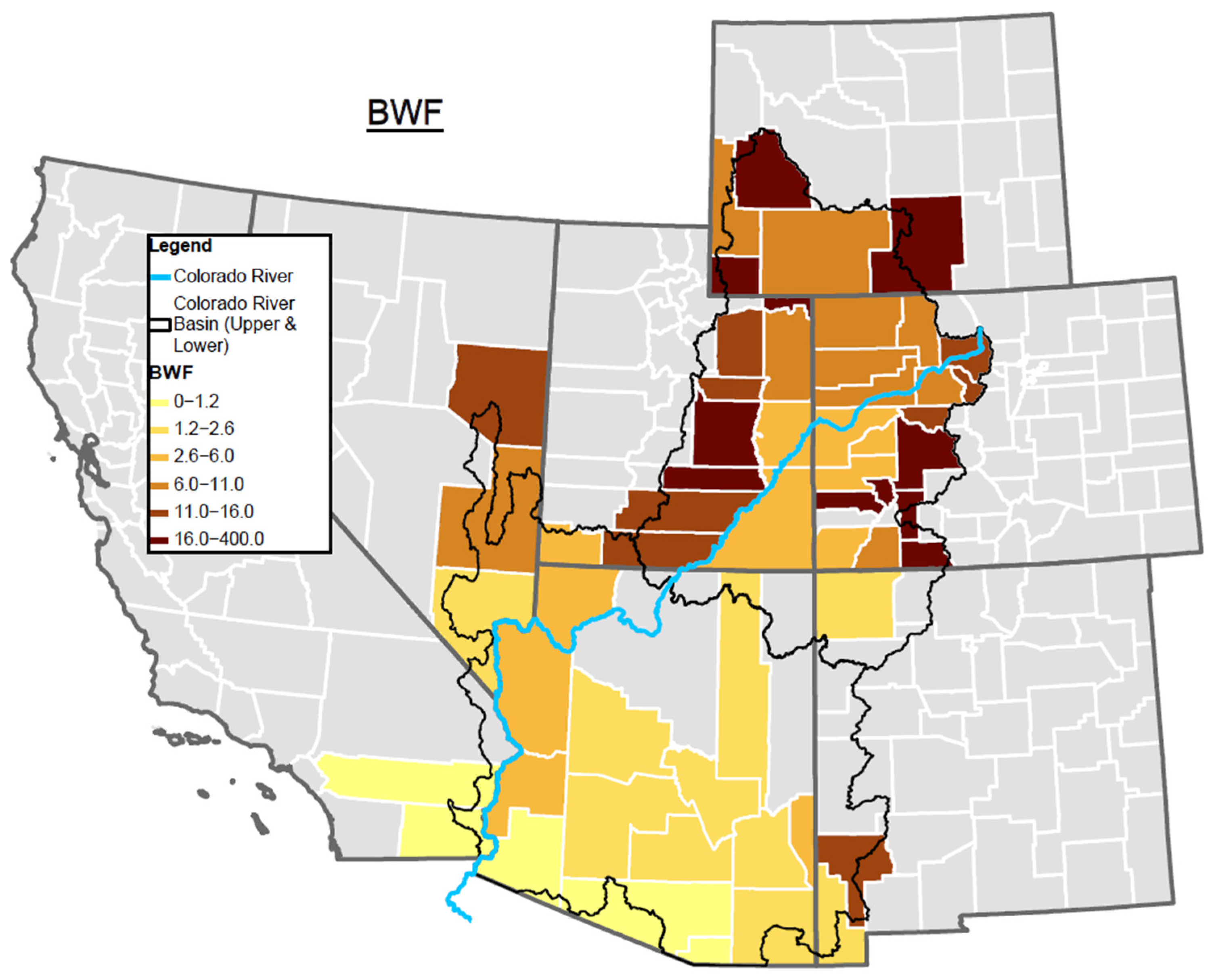
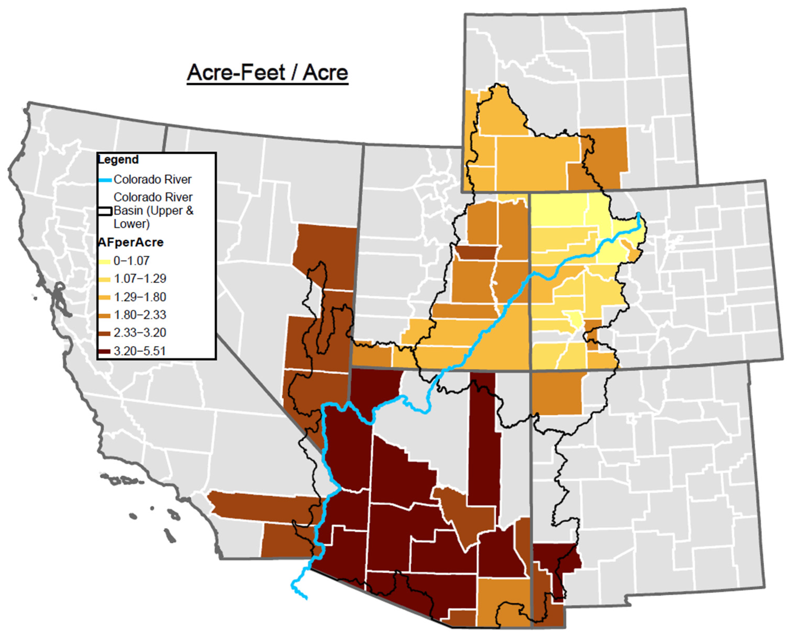
3.3. Blue Water Footprint (BWF)

The blue water footprint (BWF) is expressed here as the amount of irrigation water consumed per thousand dollars of crop revenue produced. The Basin average was 1.62 AF/USD1K (1998 m3/USD1K). The BWF averaged 1.23 AF/USD1K (1517 m3/USD1K) across Lower Basin counties and 7.63 AF/USD1K (9411 m3/USD1K) across Upper Basin counties. Water applications or consumptive use per unit of irrigated cropland are often used as metrics of water use intensity. Comparison of Figure 6 (BWF) and Figure 7 (water consumed per irrigated acre (W/Ai)), however, illustrates that water use per acre does not track especially closely with county BWFs. In fact, the two metrics are negatively correlated. The Spearman rank correlation coefficient between BWF and W/Ai is −0.52 (p = 0.00005).

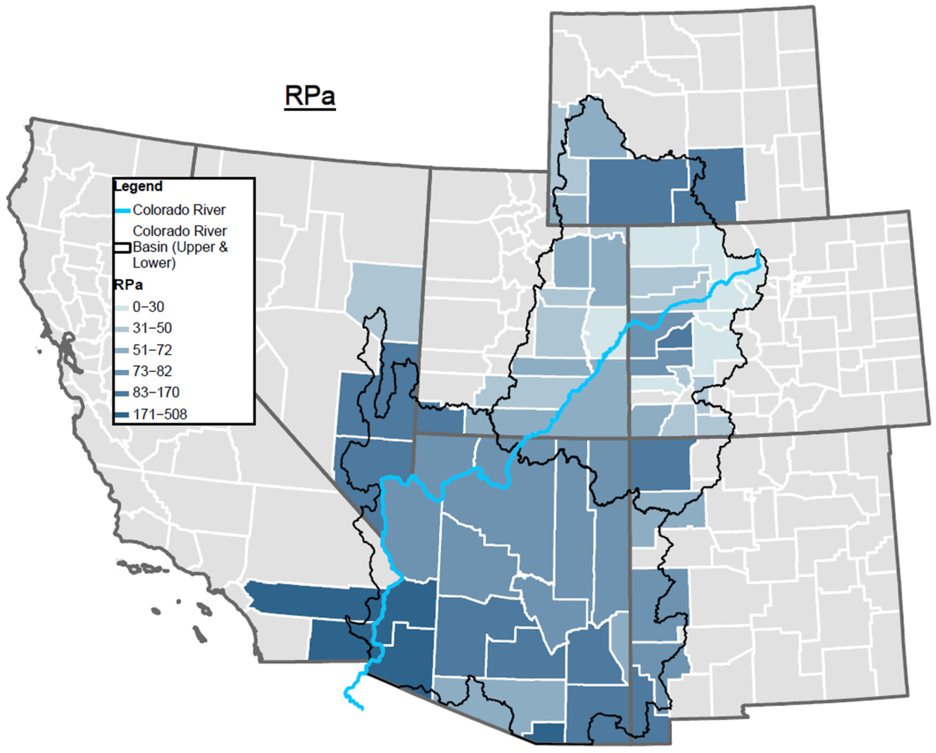
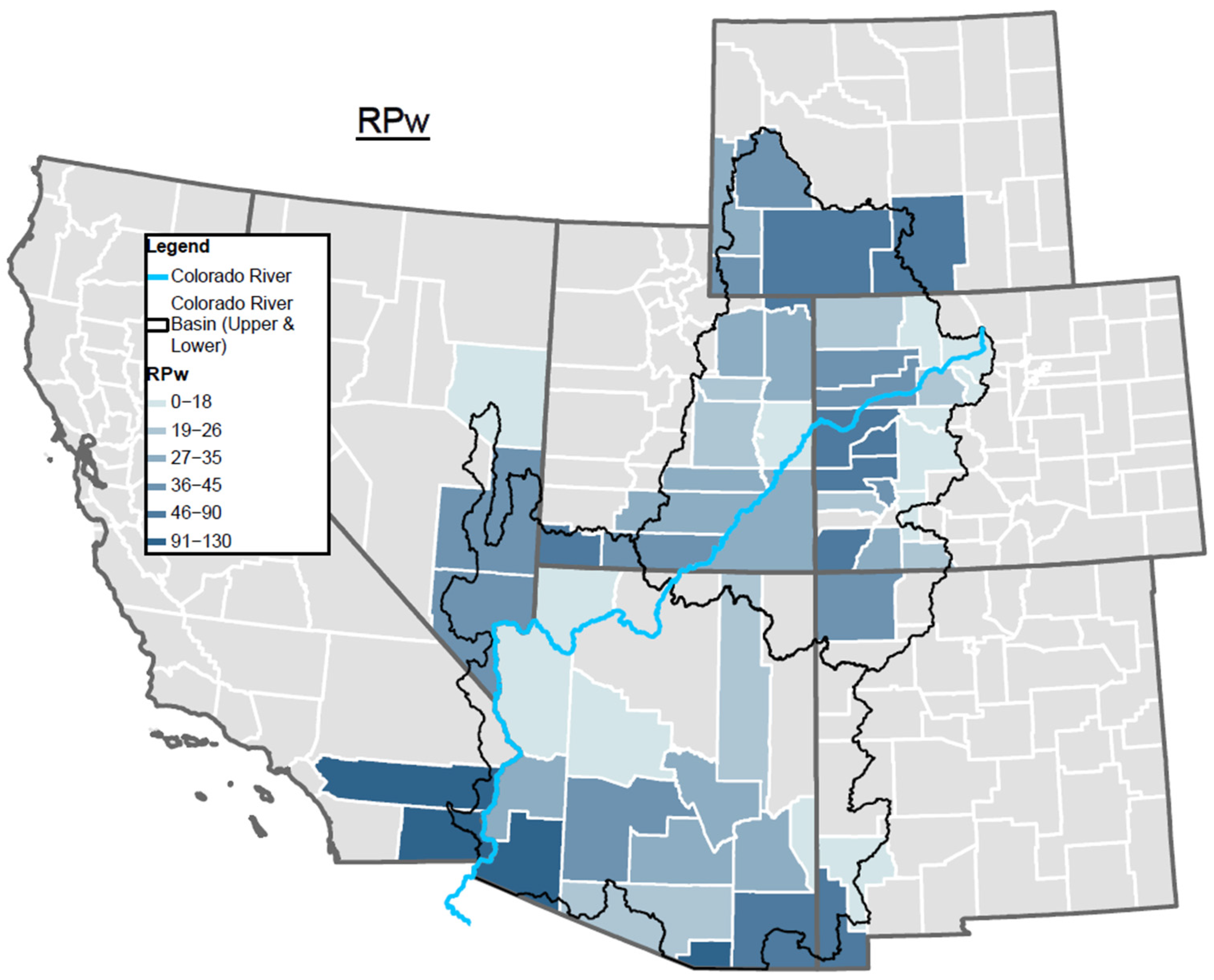
3.4. Irrigation Rent Premiums

County-level rent premiums on a per-acre basis (Figure 8) and a per-acre-foot basis (Figure 9) again reflect the general pattern (with some differences) as the other water productivity metrics. Premiums for irrigation tend to be higher in the southernmost counties of the Lower Basin, followed by premiums in the rest of the Lower Basin, then premiums in the Upper Basin. Results are more mixed for rental premiums per acre-foot (RPw). This is because some counties with high rental premiums per acre (RPa) also have crop mixes with larger water requirements. Conversely, some Upper Basin counties have lower premiums per acre, but lower water requirements. One may think of RPw as the average increase in value of rented cropland per AF of water applied. Counties with greater water requirements have lower average rent increases per quantity of water consumed, but larger water requirements (more water consumed).

3.5. Association between Water Productivity Measures

Table 2 reports the Spearman rank correlation coefficients, ρ, for the reported water productivity measures. BWF is the reciprocal of EWPg so perfectly negatively correlated with it (ρ = −1). As noted above, water-use intensity, the water consumed per irrigated acre (W/Ai), is negatively correlated with BWF. Water-use intensity is significantly (based on p values) and positively correlated with the water productivity measures EWPg and EWPn, and the per-acre rent premium for irrigated cropland, RPa.
It is somewhat perplexing that the correlation between RPw and the other metrics is relatively weak. Intuitively, one might think that RPw and EWPn would conceptually be closely related, based on net farm income per acre-foot of water. Yet, the correlation (although statistically significant) is only 0.23. Based on inspection of the data, there do not appear to be a few outliers that significantly change the correlations. We also split the sample into Lower and Upper Basins, to explore if heterogeneity of cropping systems might be a factor. However, the correlation was weak in each basin separately. One possibility is the fact that EWPn does not net out all crop input costs and underestimates labor costs in the Upper Basin. Another factor is that RPa, is positively correlated with W/Ai. RPa is converted to RPw, by dividing it by W/Ai. This imposes a “penalty” on values of RPw in regions where W/Ai is especially large. In regions where W/Ai is large, irrigation increases the productivity of the land more, but more water is also needed to achieve that effect. More formal theoretical analysis on this issue is beyond the scope of this study, but is worth pursuing.

4. Discussion

In this study we have developed county-level measures of agricultural water productivity and identified general patterns in the spatial distribution of these measures across the Colorado River Basin. Economic water productivity, both in gross- and net-revenue terms, exhibits some of its highest values in the Basin along the Colorado River mainstem towards the southwest portion of the study area, as well as along the U.S.–Mexico border. This area, especially around the Colorado mainstem, is a center of high-value U.S. winter vegetable production [57,58]. Ref. [59] documented how Yuma County agriculture significantly increased its average EWPg by shifting from long-season crops such as cotton and alfalfa to wheat–vegetable rotations that avoided planted acres in summer months.
Cumulative distributions of water consumption in the Basin ranked by EWPn show a wide range of water productivity values, but generally a significant share of Basin-wide consumption is generating relatively low net returns per AF of water consumed. For example, roughly 2 maf (2.5 km3) is consumed, generating less than 125 USD/AF (USD 0.10/m3) (net basis) at the county level, on average.
Some advocates for water conservation in the Colorado Basin have recommended shifting to cropping systems with lower water intensity (less water consumption per area of irrigated land) [30,60,61]. Yet, other researchers have emphasized shifting to cropping systems with lower blue water footprints to address water scarcity [62,63,64,65,66]. This presents a conundrum for Colorado River Basin water conservation. In general, counties with higher water intensities have lower blue water footprints. Counties with lower water intensities have higher blue water footprints (Figure 6 and Figure 7 and Table 2). This occurs because the low-desert production environment in the southwestern portion of the Lower Basin is characterized by higher temperatures and lower rainfall, which boost crop water requirements. This low-desert environment, however, is also ideal for growing high-value vegetable crops [56]. Vegetables tend to have higher economic water productivity and a low water footprint [56,67].
Recent voluntary conservation agreements in the Colorado River Basin have achieved water savings by compensating irrigators for fallowing cropland and freeing-up water to be kept in storage in Lake Mead or Lake Powell. Between 2015 and 2018, the System Conservation Pilot Program achieved water savings of 47,280 AF (58.3 million m3) in the Upper Basin at an average cost of 180 USD/AF (USD 0.15/m3). Lower Basin conservation projects freed up 175,347 AF (216 million m3) of water at an average price of 170 USD/AF (USD 0.14/m3) [13]. The Lower Colorado River Basin System Conservation and Efficiency Program provides payments up to 400 USD/AF (USD 0.32/m3) for three-year agreements [15], while the renewed Upper Basin pilot program has base payments of 150 USD/AF (USD 0.12/m3) [16]. These differences in offered rates mirror differences this study found in EWPn measures between the Upper and Lower Basin counties. Our results suggest that nearly 2 maf (2.47 km3) of water (more than 20% of Basin agricultural consumptive use) earned an EWPn less than 100 USD/AF (USD 0.08/m3). Converting to today’s dollars would increase EWPn values by roughly 25%. Even so, this suggests that current payment rates offered for water conservation are competitive with the opportunity cost of foregone crop production in much of the Basin. The results suggest that significant water conservation may be supplied by Basin agriculture without large, Basin-scale reductions in crop cash receipts.
Voluntary agricultural conservation programs may include compensation not only for the irrigators, but for others, such as input suppliers and farm laborers in the local economy. These may suffer if lands are fallowed to conserve water. Earlier agriculture-to-urban water-transfer programs between Southern California cities and the Imperial Irrigation District and Palo Verde Irrigation District included such payments to third parties [68,69,70]. To inform similar programs in the future, EWPg based on gross crop returns may be a preferred metric. As agriculture is a competitive industry with relatively small profit margins, gross returns capture payments to input suppliers and to farm labor. EWPg may thus capture direct opportunity costs of foregoing agriculture production for irrigators, input suppliers, and farm labor [56,71].

5. Conclusions

This study has quantified the large differences in agricultural water productivity measures across different counties of the Colorado River Basin. While the challenges facing the Colorado River Basin are substantial, it is not unique in confronting water scarcity. Given the availability of appropriate data, the methods applied in this study offer a useful frame of analysis for other regions addressing pressure on limited water supplies, and may serve as a starting point in developing programs to compensate irrigators for conservation.
We note some limitations of this study, and some future research directions. First, our analysis develops water productivity at the county level. As such, the estimates are abstracted from differences in water productivity across cropping systems within counties. Intercounty differences, nevertheless, were shown to be quite large. Second, USGS county-level estimates of agricultural consumptive water use are released with long lags. Data for 2015 were not released until 2020. More up-to-date water productivity measures would be useful to inform Basin water policy. Results, though, show that irrigated-cropland cash rent premiums per acre were strongly correlated (positively) with economic water productivity (EWPg) and (negatively) with the crop blue water footprint (BWF). Data to compute cash rent premiums are annually reported with relatively short lags (less than a year). Cash rent premiums may then serve as a convenient proxy measure for other water productivity measures.
Our measure EWPn, of net farm returns per unit of water, has incomplete coverage of labor costs in the Upper Basin, while excluding fuel, machinery, and capital costs across the entire Basin. In these respects EWPn overstates net returns and, potentially, levels of compensation needed for water conservation payments. At the same time, however, the value of non-marketed hay (for feed) is a non-trivial share of output in the Basin. Failure to account for this can understate the productive value of irrigation water, and potentially underestimate levels of compensation needed for water conservation payments. It would be useful for future analysis if U.S. federal agencies charged with data collection (USDA, BEA, and the Department of Labor) could provide more complete crop-specific cost estimates.
One area of future research would be formal theoretical economic modeling to quantify relationships between water productivity, water footprints, cash rent premiums, and water-use intensity. The low correlation of rent premiums per acre-foot of water with other water productivity measures is somewhat of a puzzle, which merits further investigation.
Another future research direction would be to understand how different factors—such as climate, access to federal surface-water projects, or availability of farm labor—contribute to such wide differences. Another research area would be to explore how well cash rental rates and the irrigation premium explain differences in water leasing rates in the Colorado River Basin.

Author Contributions

Conceptualization, G.B.F.; methodology, G.B.F.; software, D.D.; validation, G.B.F. and D.D.; formal analysis, G.B.F. and D.D.; investigation, G.B.F. and D.D.; resources, G.B.F. and D.D.; data curation, G.B.F. and D.D.; writing—original draft preparation, G.B.F. and D.D.; writing—review and editing, G.B.F. and D.D.; visualization, D.D. All authors have read and agreed to the published version of the manuscript.

Funding

This research received no external funding.

Data Availability Statement

Data on crop receipts and purchased input expenses come from the U.S. Bureau of Economic Analysis (2022). CAINC45: Farm income and expenses. Retrieved from https://www.bea.gov/data/income-saving/personal-income-county-metro-and-other-areas (accessed on 27 December 2023). Data on county- and agricultural-district-level cash rents come from the U.S. Department of Agriculture (USDA), National Agricultural Statistics Service (NASS), NASS Quick Stats. Retrieved from https://quickstats.nass.usda.gov/ (accessed on 27 December 2023. Data on county-level consumptive water use for irrigation came from the US Geological Survey (USGS). Water-use data available from USGS. Retrieved from https://water.usgs.gov/watuse/data/ (accessed on 27 December 2023).

Conflicts of Interest

The authors declare no conflicts of interest.

References

  1. U.S. Bureau of Reclamation. Near-Term Colorado River Operations Revised Draft Supplemental Environmental Impact Statement. October 2023. Available online: https://www.usbr.gov/ColoradoRiverBasin/documents/NearTermColoradoRiverOperations/20231019-Near-termColoradoRiverOperations-RevisedDraftEIS-508.pdf (accessed on 25 December 2023).
  2. U.S. Bureau of Reclamation. Colorado River Compact. 1922. Available online: https://www.usbr.gov/lc/region/pao/pdfiles/crcompct.pdf (accessed on 25 December 2023).
  3. Frisvold, G.B.; Fernandez, L.M.; Lehner, F.; McAfee, S.A.; Megdal, S.; Payton, E.; Schmidt, J.; Vano, J.; Woodhouse, C. Featured Collection Introduction: Severe Sustained Drought Revisited: Managing the Colorado River System in Times of Water Shortage 25 Years Later—Part I. J. Am. Water Res. Assoc. 2022, 58, 597–603. [Google Scholar] [CrossRef]
  4. Stockton, C.W.; Jacoby, G.C. Long-Term Surface Water Supply and Streamflow Levels in the Upper Colorado River Basin; Lake Powell Research Project, Bulletin No. 18; Institute of Geophysics and Planetary Physics, University of California: Los Angeles, CA, USA, 1976; 70p. [Google Scholar]
  5. Woodhouse, C.; Gray, S.; Meko, D. Updated streamflow reconstructions for the Upper Colorado River Basin. Water Resour. Res. 2006, 42, W05415. [Google Scholar] [CrossRef]
  6. USBR (U.S Bureau of Reclamation). Colorado River Basin Natural Flow and Salt Data. 2021. Available online: https://www.usbr.gov/lc/region/g4000/NaturalFlow/provisional.html (accessed on 25 December 2023).
  7. Wheeler, K.; Udall, B.; Wang, J.; Kuhn, E.; Salehabadi, H.; Schmidt, J. What will it take to stabilize the Colorado River? Science 2022, 344, 373–375. [Google Scholar] [CrossRef] [PubMed]
  8. U.S. Department of the Interior. Record of Decision: Colorado River Interim Guidelines for Lower Basin Shortages and the Coordinated Operations for Lake Powell and Lake Mead. 2007. Available online: https://www.usbr.gov/lc/region/programs/strategies/RecordofDecision.pdf (accessed on 25 December 2023).
  9. Udall, B.; Overpeck, J. The twenty-first century Colorado River hot drought and implications for the future. Water Resour. Res. 2017, 53, 2404–2418. [Google Scholar] [CrossRef]
  10. Booker, J.F. Colorado River Water Use and Climate: Model and Application. J. Am. Water Res. Assoc. 2022, 58, 673–689. [Google Scholar] [CrossRef]
  11. Meko, D.M.; Woodhouse, C.A.; Winitsky, A.G. Tree-ring perspectives on the Colorado River: Looking back and moving forward. J. Am. Water Res. Assoc. 2022, 58, 604–621. [Google Scholar] [CrossRef]
  12. Pierce, D.W.; Cayan, D.R.; Goodrich, J.; Das, T.; Munévar, A. Evaluating global climate models for hydrological studies of the upper Colorado River Basin. J. Am. Water Res. Assoc. 2022, 58, 709–734. [Google Scholar] [CrossRef]
  13. U.S Bureau of Reclamation. USBR Pilot Projects to Increase Colorado River System Water in Lake Powell and Lake Mead; Report to the US Congress. 2021. Available online: https://www.usbr.gov/lc/region/programs/PilotSysConsProg/report_to_congressW_appendices2021.pdf (accessed on 25 December 2023).
  14. U.S Bureau of Reclamation. Colorado River Basin Drought Contingency Plans. 2023. Available online: https://www.usbr.gov/dcp/finaldocs.html (accessed on 25 December 2023).
  15. Stern, C.; Sheikh, P.; Hite, K. Management of the Colorado River: Water Allocations, Drought, and the Federal Role. Congressional Research Service Report R45546 Version 37. Updated 1 November 2023. Available online: https://sgp.fas.org/crs/misc/R45546.pdf (accessed on 25 December 2023).
  16. Upper Colorado River Commission. System Conservation Pilot Program. 2023. Available online: http://www.ucrcommission.com/system-conservation-pilot-program-for-2023 (accessed on 11 August 2023).
  17. The Colorado River Basin States Representatives of Arizona, California, and Nevada. Lower Basin Plan Letter to USBR. 22 May 2023. Available online: https://www.doi.gov/sites/doi.gov/files/lower-basin-plan-letter-5-22-2023.pdf (accessed on 25 December 2023).
  18. U.S. Bureau of Reclamation. Colorado River Basin Water Supply and Demand Study Technical Report C Water Demand Assessment. Available online: https://www.usbr.gov/lc/region/programs/crbstudy/finalreport/techrptC.html (accessed on 25 December 2023).
  19. Harou, J.J.; Medellín-Azuara, J.; Zhu, T.; Tanaka, S.K.; Lund, J.R.; Stine, S.; Olivares, M.A.; Jenkins, M.W. Economic consequences of optimized water management for a prolonged, severe drought in California. Water Resour. Res. 2010, 46, W05522. [Google Scholar] [CrossRef]
  20. Medellín-Azuara, J.; Harou, J.J.; Olivares, M.A.; Madani, K.; Lund, J.R.; Howitt, R.E.; Tanaka, S.K.; Jenkins, M.W. Adaptability and adaptations of California’s water supply system to dry climate warming. Clim. Chang. 2008, 87 (Suppl. 1), S75–S90. [Google Scholar] [CrossRef]
  21. Tanaka, S.K.; Zhu, T.; Lund, J.R.; Howitt, R.E.; Jenkins, M.W.; Pulido-Velazquez, M.; Tauber, M.; Ritzema, R.S.; Ferreira, I.C. Climate warming and water management adaptation for California. Clim. Chang. 2006, 76, 361–387. [Google Scholar] [CrossRef]
  22. Frisvold, G.B.; Jackson, L.E.; Pritchett, J.G.; Ritten, J.P.; Svoboda, M. Agriculture and ranching. In Assessment of Climate Change in the Southwest United States: A Report Prepared for the National Climate Assessment; Island Press: Washington, DC, USA, 2013; pp. 218–239. [Google Scholar]
  23. U.S. Bureau of Reclamation. Upper Colorado River Basin: Consumptive Uses and Losses 2016–2020. Available online: https://www.usbr.gov/uc/DocLibrary/Reports/ConsumptiveUsesLosses/20220214-ProvisionalUpperColoradoRiverBasin2016-2020-CULReport-508-UCRO.pdf (accessed on 25 December 2023).
  24. Dieter, C.A.; Maupin, M.A.; Caldwell, R.R.; Harris, M.A.; Ivahnenko, T.I.; Lovelace, J.K.; Barber, N.L.; Linsey, K.S. Estimated Use of Water in the United States in 2015; U.S. Geological Survey Circular 1441; U.S. Government Printing Office: Washington, DC, USA, 2018; 65p.
  25. Goemans, C.; Pritchett, J. Western water markets: Effectiveness and efficiency. In Water Markets for the 21st Century: What Have We Learned? Easter, K.W., Huang, Q., Eds.; Springer: Dordrecht, The Netherlands, 2014; pp. 305–330. [Google Scholar]
  26. Nichols, P.D.; Murphy, M.K.; Kenney, D.S. Water and Growth in Colorado. A Review of Legal and Policy Issues; Natural Resources Law Center, University of Colorado: Boulder, CO, USA, 2001. [Google Scholar]
  27. Howe, C.W.; Schurmeier, D.R.; Shaw, W.D., Jr. Innovative approaches to water allocation: The potential for water markets. Water Resour. Res. 1986, 22, 439–445. [Google Scholar] [CrossRef]
  28. Young, R.A.; Loomis, J.B. Determining the Economic Value of Water: Concepts and Methods; Routledge: New York, NY, 2014. [Google Scholar]
  29. Ayres, A.; Adams, T.; Carron, J.; Cohen, M.; Saracino, A. Potential impacts of reduced inflows to the Salton Sea: Forecasting non-market damages. J. Am. Water Res. Assoc. 2022, 58, 1128–1148. [Google Scholar] [CrossRef]
  30. Cohen, M.; Christian-Smith, J.; Berggren, J. Water to Supply the Land: Irrigated Agriculture in the Colorado River Basin; Pacific Institute: Oakland, CA, USA, 2013; Available online: https://pacinst.org/wp-content/uploads/2013/05/pacinst-crb-ag-1.pdf (accessed on 25 December 2023).
  31. Hansen, K.; Coupal, R.; Yeatman, E.; Bennett, D. Economic Assessment of a Water Demand Management Program in the Wyoming Colorado River Basin; University of Wyoming Extension: Laramie, WY, USA, 2021. [Google Scholar]
  32. U.S. Department of Agriculture (USDA), National Agricultural Statistics Service (NASS). NASS Quick Stats. Available online: https://quickstats.nass.usda.gov/ (accessed on 25 December 2023).
  33. U.S. Bureau of Economic Analysis (BEA). CAINC45 Farm Income and Expenses. 2022. Available online: https://www.bea.gov/data/income-saving/personal-income-county-metro-and-other-areas (accessed on 25 December 2023).
  34. US Geological Survey (USGS). Water-Use Data Available from USGS. Available online: https://water.usgs.gov/watuse/data/ (accessed on 25 December 2023).
  35. Senay, G.B.; Bohms, S.; Singh, R.K.; Gowda, P.H.; Velpuri, N.M.; Alemu, H.; Verdin, J.P. Operational evapotranspiration mapping using remote sensing and weather datasets—A new parameterization for the SSEB approach. J. Am. Water Resour. Assoc. 2013, 49, 577–591. [Google Scholar] [CrossRef]
  36. Booker, J.F.; Trees, W.S. Implications of water scarcity for water productivity and farm labor. Water 2020, 12, 308. [Google Scholar] [CrossRef]
  37. U.S. Bureau of Labor Statistics. Quarterly Census of Employment and Wages (QCEW). 2023. Available online: https://www.bls.gov/cew/ (accessed on 25 December 2023).
  38. U.S. Bureau of Economic Analysis (BEA). Local Area Personal Income and Employment Methodology. 2017. Available online: https://www.bea.gov/sites/default/files/methodologies/lapi2016.pdf (accessed on 25 December 2023).
  39. Mekonnen, M.; Hoekstra, A. The green, blue and grey water footprint of crops and derived crop products. Hydrol. Earth Syst. Sci. 2011, 15, 1577–1600. [Google Scholar] [CrossRef]
  40. Mekonnen, M.; Gerbens-Leenes, W. The water footprint of global food production. Water 2020, 12, 2696. [Google Scholar] [CrossRef]
  41. Konar, M.; Marston, L. The water footprint of the United States. Water 2020, 12, 3286. [Google Scholar] [CrossRef]
  42. Roson, R.; Sartori, M. A decomposition and comparison analysis of international water footprint time series. Sustainability 2015, 7, 5304–5320. [Google Scholar] [CrossRef]
  43. Mekonnen, M.; Hoekstra, A. National Water Footprint Accounts: The Green, Blue and Grey Water Footprint of Production and Consumption; Value of Water Research Report Series No. 50; UNESCO-IHE: Delft, The Netherlands, 2011. [Google Scholar]
  44. Supalla, R.; Buell, T.; McMullen, B. Economic and State Budget Cost of Reducing the Consumptive Use of Irrigation Water in the Platte and Republican Basins; University of Nebraska-Lincoln, Department of Agricultural Economics, for the Nebraska Department of Natural Resources: Lincoln, NE, USA, 2006. [Google Scholar]
  45. Henderson, J.; Akers, M. Can markets improve water allocation in rural America? Fed. Res. Bank Kansas City Econ. Rev. 2008, 93, 97–119. [Google Scholar]
  46. Thompson, C.L.; Supalla, R. Understanding the Value of Water in Nebraska: Future Expectations and Considerations. Cornhusker Economics. 15 December 2010. Available online: https://digitalcommons.unl.edu/agecon_cornhusker/510 (accessed on 25 December 2023).
  47. Pritchett, J.; Thorvaldson, J.; Frasier, M. Water as a crop: Limited irrigation and water leasing in Colorado. Rev. Agric. Econ. 2008, 30, 435–444. [Google Scholar] [CrossRef]
  48. Rimsaite, R.; Gibson, J.; Brozović, N. Informing drought mitigation policy by estimating the value of water for crop production. Environ. Res. Commun. 2021, 3, 041004. [Google Scholar] [CrossRef]
  49. Paulson, N.; Schnitkey, G.; Baltz, J.; Zulauf, C. Information for Setting 2024 Cash Rents. Farmdoc Daily 2023, 13, 160. [Google Scholar]
  50. Carson, N.; Langemeier, M. Relationship between cash rent and net return to land in Indiana. J. ASFMR 2019, 1, 126–131. [Google Scholar]
  51. Featherstone, A.M.; Taylor, M.R.; Gibson, H. Forecasting Kansas land values using net farm income. Agric. Financ. Rev. 2017, 77, 137–152. [Google Scholar] [CrossRef]
  52. Fei, C.; Hogan, J.R.; McCarl, B.; Vargas, A.; Yang, Y. Water Values in South Central Texas; An Output from the NSF Project Addressing Innovations at the Nexus of Food, Energy, and Water Systems-1639327; Department of Agricultural Economics, Texas A & M University: College Station, TX, USA, 2016. [Google Scholar]
  53. Veettil, A.V.; Mishra, A.K. Water security assessment using blue and green water footprint concepts. J. Hydrol. 2016, 542, 589–602. [Google Scholar] [CrossRef]
  54. Xu, H.; Wu, M. A first estimation of county-based green water availability and its implications for agriculture and bioenergy production in the United States. Water 2018, 10, 148. [Google Scholar] [CrossRef]
  55. Yun, S.D.; Gramig, B.M. Agro-climatic data by county: A spatially and temporally consistent US dataset for agricultural yields, weather and soils. Data 2019, 4, 66. [Google Scholar] [CrossRef]
  56. Bickel, A.K.; Duval, D.; Frisvold, G.B. Simple approaches to examine economic impacts of water reallocations from agriculture. J. Contemp. Water Res. Educ. 2019, 168, 29–48. [Google Scholar] [CrossRef]
  57. Kerna, A.; Duval, D.; Frisvold, G. Arizona Leafy Greens: Economic Contributions of the Industry Cluster 2015 Economic Contribution Analysis; University of Arizona: Tucson, AZ, USA, 2017. [Google Scholar]
  58. Kerna, A.; Duval, D.; Frisvold, G.; Uddin, A. The Contribution of Arizona’s Vegetables and Melon Industry Cluster to the State Economy; University of Arizona: Tucson, AZ, USA, 2015. [Google Scholar]
  59. Frisvold, G.; Sanchez, C.; Gollehon, N.; Megdal, S.B.; Brown, P. Evaluating gravity-flow irrigation with lessons from Yuma, Arizona, USA. Sustainability 2018, 10, 1548. [Google Scholar] [CrossRef]
  60. Postel, S.L.; Morrison, J.I.; Gleick, P.H. Allocating fresh water to aquatic ecosystems: The case of the Colorado River Delta. Water Int. 1998, 23, 119–125. [Google Scholar] [CrossRef]
  61. Nabhan, G.P.; Richter, B.D.; Riordan, E.C.; Tornbom, C. Toward Water-Resilient Agriculture in Arizona: Future Scenarios Addressing Water Scarcity; Lincoln Institute of Land Policy: Cambridge, MA, USA, 2023. [Google Scholar]
  62. Almazán-Gómez, M.A.; Duarte, R.; Langarita, R.; Sánchez-Chóliz, J. Effects of water re-allocation in the Ebro river basin: A multiregional input-output and geographical analysis. J. Environ. Manag. 2019, 241, 645–657. [Google Scholar] [CrossRef] [PubMed]
  63. Salmoral, G.; Carbo, A.V.; Zegarra, E.; Knox, J.W.; Rey, D. Reconciling irrigation demands for agricultural expansion with environmental sustainability-A preliminary assessment for the Ica Valley, Peru. J. Clean. Prod. 2020, 276, 123544. [Google Scholar] [CrossRef]
  64. Huang, H.; Xie, P.; Duan, Y.; Wu, P.; Zhuo, L. Cropping pattern optimization considering water shadow price and virtual water flows: A case study of Yellow River Basin in China. Agric. Water Manag. 2023, 284, 108339. [Google Scholar] [CrossRef]
  65. Pahlow, M.; Snowball, J.; Fraser, G. Water footprint assessment to inform water management and policy making in South Africa. Water SA 2015, 41, 300–313. [Google Scholar] [CrossRef]
  66. Bulut, A.P. Determining the water footprint of sunflower in Turkey and creating digital maps for sustainable agricultural water management. Environ. Dev. Sustain. 2023, 25, 11999–12010. [Google Scholar] [CrossRef]
  67. Molden, D.; Oweis, T.; Steduto, P.; Bindraban, P.; Hanjra, M.A.; Kijne, J. Improving agricultural water productivity: Between optimism and caution. Agric. Water Manag. 2010, 97, 528–535. [Google Scholar] [CrossRef]
  68. Ayres, A.; Bigelow, D. Engaging irrigation districts in water markets. In The Future of Water Markets: Obstacles and Opportunities; Edwards, E., Regan, S., Eds.; Property and Environment Research Center (PERC): Bozeman, MT, USA, 2022; pp. 53–62. [Google Scholar]
  69. Bark, R.H.; Frisvold, G.; Flessa, K.W. The role of economics in transboundary restoration water management in the Colorado River Delta. Water Resour. Econ. 2014, 8, 43–56. [Google Scholar] [CrossRef]
  70. Howitt, R.; Hanak, E. Incremental water market development: The California water sector 1985–2004. Can. Water Resour. J. 2005, 30, 73–82. [Google Scholar] [CrossRef]
  71. Sunding, D.; Zilberman, D.; MacDougall, N. Water markets and the cost of improving water quality in the San Francisco Bay/Delta Estuary. Hastings West-Nowest J. Environ. Law Policy 1995, 2, 159–165. [Google Scholar]
Figure 1. Colorado River Basin States and Counties in the Study area.
Hydrology 11 00005 g001
Figure 2. Economic Water Productivity, gross return basis (EWPg) for Colorado Basin counties.
Hydrology 11 00005 g002
Figure 3. Average and marginal Economic Water Productivity, gross revenue basis (EWPg) in the Colorado River Basin.
Hydrology 11 00005 g003
Figure 4. Economic Water Productivity, net return basis (EWPn) for Colorado Basin counties.
Hydrology 11 00005 g004
Figure 5. Average and marginal Economic Water Productivity, net revenue basis (EWPn) in the Colorado River Basin.
Hydrology 11 00005 g005
Figure 6. The Blue Water Footprint (BWF)) for crop production among Colorado Basin counties.
Hydrology 11 00005 g006
Figure 7. Water-use intensity (acre-feet of water consumed per acre) for crop production among Colorado Basin counties.
Hydrology 11 00005 g007
Figure 8. Cropland cash rent premiums for irrigated land (per-acre basis) for Colorado Basin counties.
Hydrology 11 00005 g008
Figure 9. Cropland cash rent premiums for irrigated land (per acre-foot of water basis) for Colorado Basin counties.
Hydrology 11 00005 g009
Table 1. Distribution of agricultural water consumption and crop receipts in Colorado Basin counties.
Cumulative Percent of Basin Agriculural
Water Consumed
Corresponding Percent of Basin
Crop Receipts
24%49%
41%74%
52%84%
66%93%
75%97%
Table 2. Spearman rank correlations among water productivity measures.
Rent Premium
per Acre
RPa
Rent Premium
per Acre-Foot
RPw
Economic Water Productivity (Gross Returns) EWPgBlue Water Footprint BWFEconomic Water Productivity (Net Returns) EWPn
RPw0.71 §
EWPg0.68 §0.36
BWF−0.68 §−0.36 −1.00 §
EWPn0.49 §0.23 *0.78 §−0.78 §
W/Ai **0.68 §0.050.52 §−0.52 §0.41
§ p < 0.001;  p < 0.01; * p < 0.05; ** Acre-feet of water consumed per irrigated acre.
Disclaimer/Publisher’s Note: The statements, opinions and data contained in all publications are solely those of the individual author(s) and contributor(s) and not of MDPI and/or the editor(s). MDPI and/or the editor(s) disclaim responsibility for any injury to people or property resulting from any ideas, methods, instructions or products referred to in the content.

