Assimilating Soil Moisture Information to Improve the Performance of SWAT Hydrological Model

Abstract

The present work aims to highlight the possibility of improving model performance by assimilating soil moisture information in the calibration and validation process. The Soil and Water Assessment Tool (SWAT) within QGIS, i.e., QSWAT, was used to simulate the hydrological processes within the test basin, i.e., Vosvozis River Basin (VRB) in NE Greece. The model calibration and validation were conducted via SWAT-CUP for a four-year period from 2019 to 2022, in three different ways, i.e., using the traditional calibration process with river flow measurements, using satellite-based soil moisture only in the calibration, and finally incorporating satellite-based soil moisture datasets and calibrating using simultaneously flow and soil moisture information. All modeling approaches used the same set of input data related to topography, land cover, and soil information. This study utilized the recently released global scale daily downscaled soil moisture at 1 km from the Soil Moisture Active Passive (SMAP) mission to generate soil moisture datasets. Two performance indicators were evaluated: Nash Sutcliffe (NS) and coefficient of determination (R²). Results showed that QSWAT successfully simulated river flow in VRB with NS = 0.61 and R² = 0.69 for the calibration process using river flow measurements at the outlet of VRB. However, comparing satellite-based soil moisture, NS and R² were considerably lower with an average derived from the 19 subbasins (NS = 0.55, R² = 0.66), indicating lower performance related to the simulation of soil moisture regime. Subsequently, introducing satellite-derived soil moisture as an additional parameter in the calibration process along with flow improved the acquired average soil moisture results of the 19 subbasins (NS = 0.85, R² = 0.91), while preserving the satisfactory performance related to flow simulation (NS = 0.57, R² = 0.66). Our work thus demonstrates how assimilating available satellite-derived soil moisture information into the SWAT model may offer considerable improvement in the description of soil moisture conditions, keeping the satisfactory performance in flow simulation.

1. Introduction

Hydrological models are valuable scientific tools enabling the nowcasting and forecasting of various hydrological components [1]. They also contribute to the mitigation of extreme natural events like droughts and floods, through operational forecasting [2,3,4,5]. Hydrological models have become very popular also as decision-making instruments, thus helping form policies for urban planning, crop yield protection, and emergency services management, as well as towards increasing public resilience to climate change impacts [1,6]. Physically based distributed hydrological models are considered the most reliable tool for accurate predictions when there is available information at a high spatial resolution to allow for decent model parameterization. The high variability of hydrological parameters affects the rainfall–runoff relationship in river basins and therefore surface parameters need to be considered in hydrological modeling [7]. Thus, input data of the hydrological topographical characteristics, soil properties, land cover, and other hydrological parameters are required at sufficiently high spatial resolution, thus enabling the simulation of even very large and complex basins [8]. However, computational effort, data scarcity, and lack of information for reliable model parameter estimation often restrict to smaller catchments the application of such physically based models, like MIKE SHE [9,10], HYDRUS-1d, 2d, 3d [11,12,13], or ParFlow [14]. One possible solution is to simplify the complex physical system by disaggregating the basin area into smaller homogeneous hydrological units, usually known as Hydrologic Response Units [15], converting the modeling process to a semi-distributed approach. An even simpler approach, known as lumped hydrological modeling, is to consider the entire study basin as a single unit, simulating runoff as a function of the lumped catchment hydraulic properties. Results of a comparative study of three hydrological models of different complexity [16], one fully distributed, one semi-distributed, and a lumped one, indicated that many times simpler models are preferred over the fully distributed ones, due to insufficient high-resolution spatial information to evaluate the parameters of the model and the computational complexity of long-term simulations with a fully distributed model [5,16,17].

Soil and Water Assessment Tool (SWAT) [18] is a semi-distributed model developed to simulate all components of the water budget, as well as sediment yield, and water quality, and also evaluate non-point sources of pollution [8,19]. SWAT is a quasi-physically based hydrological model which evaluates the hydrologic balance at the Hydrological Response Unit (HRU) level. HRUs are a subdivision of the watershed that represents homogeneous spatial entities in terms of land use, management, and soil types. In that way, SWAT offers a computationally efficient alternative that provides continuous basin-scale simulations for long time periods. Thus, it evaluates how precipitation water (but also snowmelt and irrigation water) is partitioned among various receivers such as interception from the canopy, surface runoff, infiltration, evapotranspiration, water in the unsaturated zone, return flow from shallow aquifers, lateral subsurface flow from the soil layer and percolation to deep subsurface. SWAT has been extensively applied and validated in many areas around the globe and was found to be an efficient tool for basin scale simulations when accurate precipitation data are provided and there is the availability of observation data to calibrate the water budget [19,20]. Accordingly, [21] used the SWAT model in order to demonstrate the Al-Adhaim River runoff flow (northeast of Iraq). The model was calibrated with daily flows measured between 1 January 1983 and 31 September 1984 and validated between 1 January 1985 and 31 September 1985, with satisfactory results. The R², NS, and root mean square error (RMSE) were 0.76, 0.75, and 0.5, respectively, for calibration and 0.71, 0.69, and 0.55 for validation. In that work, the calibrated model was run over a long period (1986–2013) to estimate the relationship between changes in land cover/land use (LC/LU) and runoff.

Farhan and Thamiry [22], made a study located in the western part of Iraq. They tried to use the Arc SWAT tool in the simulation procedure to evaluate the runoff over the long-term period (1981–2019) using SWAT-CUP software, version 2012, to calibrate flow rates recorded at two gauge stations. The SWAT model for Al-Mohammadi Valley was calibrated and validated with NS = 0.72 and R² = 0.76 for the calibration process and NS = 0.63 and R² = 0.65 for the validation process, indicating excellent performance from the calculated performance indicators. Results indicated a very good performance with the maximum daily flow discharge for the study period reaching 160 m³/s for the Al-Mohammadi Valley.

While in most cases SWAT is applied for runoff estimation, ref. [23] used SWAT to obtain daily evapotranspiration values (ET) in a study area with irrigated crops in Texas High Plains. In that work, it turned out that SWAT simulates well both the daily and the average monthly ET within irrigated cultivated areas. Limitations were highlighted in the case of low irrigation conditions, especially in cotton and sunflower crops, attributed to the plant development model and associated plant parameter values within the crop database embedded in SWAT.

Although there are numerous works focusing on the accurate simulation of surface runoff and on the effects of land use/land cover and climate changes on flow regime, there are considerably fewer studies dealing with the accurate representation of soil moisture (SM) regime. SM is a hydrological parameter of particular importance for various aspects of human life and the environment. Drought conditions can be quantified using SM data, helping thus minimize their negative social and economic impacts [24]. Moreover, SM has also been identified as one of the most important factors influencing wildfire occurrence and spread [25,26], but its accurate characterization is also a key aspect for effective flood forecasting and sustainable water resources management [27]. Researchers have recently started their attempts to improve hydrological simulations using remote sensing SM products, but it is difficult to reach a ubiquitous conclusion since the performance of a hydrological model depends on many factors like the type of data used, the area being studied, how the data are evaluated, the models and the methods used for adjustment and integration [28]. For example, SWAT was applied to simulate soil water content in three different test sites in Northeast Indiana, at Bushland, Texas, and at Greeley, Colorado [29]. Results indicated that although in all three cases, the SWAT model performed satisfactorily regarding streamflow or ET simulation, there was significant uncertainty related to the characterization of SM conditions, merely due to the uncertainties in the description of soil properties but also due to the inherent uncertainty of SWAT in explaining the movement of water in the unsaturated zone. In other works however, SWAT-simulated SM was found to be in good agreement with indirect Landsat-derived SM estimates [30], keeping in mind however, that very limited in situ measurements were used to test simulated SM conditions.

A simple approach was adopted in the work of [31], where a bucket model was developed to improve the spatial resolution of a ground monitoring SM network, using 10 km precipitation from the North American Land Data Assimilation System (NLDAS). Results indicated that after calibrating the model using the in situ sensors, it could simulate SM with reasonable accuracy.

A considerable improvement in SWAT model performance was found after calibration with daily SM measurements [32], in Mundaú River Basin in Northeastern Brazil. In that work, the SWAT tool was used in order to evaluate the impacts of utilizing both the discharge and the SM datasets on model instabilities and forecasts. Among their results, they found that the NS for streamflow calibration ranges from 0.71 to 0.92 in the annual timestep among the several gauge stations. Moreover, the NS ranges between 0.55 and 0.78 in the monthly timestep. In contrast, the NS values for validation ranged from 0.53 to 0.76 for the annual time step and from 0.62 to 0.72 for the monthly time step. Calibration and validation against the daily SM dataset resulted in NS values of 0.53 and 0.52 and PBIAS of 0.4% and −1.1%, respectively. Although the results show good performance for the discharge and SM datasets, there are still some uncertainties in the calibration and validation procedure, especially when discharge data are scarce.

Another research work dealing with the simulation of SM is that of [33], where the Dutch National Hydrological Model was used to simulate SM in the Twente region, in East Netherlands, where a network of 20 SM sensors operates. In this case, however, the modeling of SM aimed primarily at upscaling the point SM measurement to the SMAP pixel area, in order to validate the SMAP SM retrievals. They concluded that after removing the data corresponding to frozen conditions and antecedent rainfall to avoid the underestimating and overstating errors associated with soil freezing and dry spells, a satisfactory unbiased root mean squared error (uRMSE) was found (0.043 m³/m³).

In another research work [34], a module for the SWAT model was created based on a combination of energy-balance rain-on-snow and physically based soil temperature. The module was applied to the South Saskatchewan River Basin. They calibrated both the SWAT base model and the SWAT-modified model utilizing daily measurements of soil water content and soil temperature at the HRU level from 2015 until 2020. Via the SUFI-2 procedure in SWAT-CUP, they found the parameters with the most critical impact (p < 0.5) on SM, snowmelt, and streamflow. Furthermore, NS efficiency in the new module was improved from 0.39 to 0.71 and from 0.42 to 0.76 for calibration and validation procedures, respectively. Additionally, they found that for SWAT-simulated daily soil water content, the measured data were closer to that estimated with SWAT modified against SWAT base output. Moreover, SWAT-modified results matched the observations better than the SWAT base values and field measurements did. Among their study results, it was found that the SWAT base underestimated the soil temperature within cold seasons, while the SWAT modification essentially improved the simulation of the soil temperature for winters. The SWAT module captured the snow cover impact on surface soil ice-water quantity. Finally, the spatial analysis indicated that in the western part of the South Saskatchewan River Basin, the SWAT-modified model anticipates higher soil water content and lower soil temperature in contrast with the eastern part where the SWAT base model predicted exactly the opposite.

While model SM predictions are updated via independent observations by utilizing data assimilation procedures, effects on predicted crop yield and water quality remain uncertain. An evaluation of data assimilation impacts for several forecasts in SWAT was conducted by [35]. They used satellite surface SM data series from the SMAP mission in order to improve SWAT SM. Their study took place in the U.S. for two experimental watersheds. Among their study results, it was found that the two watersheds illustrated that data assimilation significantly affected both crop yield and water quality forecasts. Although, soil percolation algorithm modification did not make the results of assimilation better. An increase in median SM from 2% to 6% was the outcome of assimilation, something that made the total daily streamflow increase from 0.43 to 1.70 m³/s. Crop yield forecasts were affected by data assimilation from nutrient and water availability changes. Finally, they conclude that crop yield predictions to SM updates prove that assimilation can affect model predictions.

SM and other satellite-based data were used in the study by [36]. More specifically, the European Space Agency (ESA) Climate Change Initiative SM dataset (CCI SM), based on the Soil Water Index, in combination with discharge observations was used in their study in order to model a large-scale river basin called Odra. The Odra River basin is located in Central Europe and drains into the Baltic Sea. They used river discharge measurements of 26 stations and the CCI SM dataset (for the entire soil profile and topsoil) over 1476 subbasins, in order to calibrate their model via SWAT for a period from 1997 to 2019. They chose the Kling–Gupta efficiency (KGE) index as a runoff calibration objective function, while for the SM calibration objective function, they used the Spatial Efficiency (SPAEF) index. They finally tried two calibration techniques, one of them involved only discharge information, and the other involved simultaneously both discharge and satellite-based SM data. From the comparison of the two strategies, they concluded that in the first approach, the average KGE for discharge was >0.60, while in the second one, KGE was equal to 0.67. Among their study results, it was found that SPAEF values indicated that SWAT+ has accepted accuracy in the simulation process of SM. Moreover, it was also highlighted that calibration with the second strategy improves the accuracy of the simulation of crop yield. Their study indicated that the inclusion of satellite-derived SM in the calibration process may enhance the precision and uniformity of agro-hydrological modeling within the concerned river basin.

A multi-step calibration approach has been recently presented in [1], applying the SWAT model in Petzenkirchen in the western part of Lower Austria. They introduced a sequential calibration method, which provided better performance on different hydrological components and procedures. The calibration method started with surface runoff and groundwater flow, then continued with product yield and SM, and finally, the model was calibrated with total runoff and sediment yield, respectively. Calibration and validation were performed using the SWAT-plusR r-package. Results revealed that the model attained the capability to predict groundwater flow, surface runoff, SM content, total runoff, and sediment yield with NS > 0.75. Moreover, the simulation of crop yields was satisfactory with a PBIAS extending from −17% to 14%. The calibration of the surface runoff had the highest influence on the streamflow output and improved the NS from 0.39 to 0.77. Results indicated that the stepwise calibration is more precise than the simulated ones and better represents the different hydrologic factors and procedures.

Other parameters, like snow water equivalent in snow-dominated basins, have also been subject to multi-objective calibration procedures, like the one presented for the Upper Adige River basin, in Northeastern Italian Alps [37]. In that work, the suitability of the SWAT model to obtain realistic river flow and snow water equivalent estimates using the multi-objective approach was highlighted.

In the research of [28], a review of past studies on using a combination of remote sensing and global datasets in hydrological modeling that is spread out across multiple locations is presented. The analysis looked into how these data sets are used in different places and sizes. Furthermore, several articles were analyzed in order to identify how researchers work together. The research further divided the analysis into different types of information, such as rainfall, a digital elevation model, land use, soil distribution, leaf area index, snow-covered area, evapotranspiration, SM, and temperature. The results showed that choosing the correct datasets is really important while validating with ground measurements is also very useful and will greatly affect model performance. This research provides helpful information about using satellite images and global data to study water systems.

In the present work, the SWAT model was tested for its performance to describe various hydrological components in VRB in NE Greece (Figure 1), calibrating it in a three-fold way within SWAT-CUP; initially, river gauge measurements were used for calibration, and then the model was calibrated against satellite-based SM retrievals, while a simultaneous calibration using both river gauge measurements and satellite-derived SM data was also attempted. Results indicated an improvement in the description of the SM regime without compromising the surface runoff SWAT output, thus highlighting the usefulness of SM calibration in the modeling process. To the best of our knowledge, it is the first time that such an analysis was conducted regarding SM, and this is a certain novelty of this work as it provides a methodological approach for the improvement of the description of the SM regime. The work is structured with the study area description namely VRB, the selected software description namely the SWAT model, and the SWAT input data description such as the ASTER GDEM V3, the CORINE land cover, soil, and weather information are analyzed. Moreover, an analysis of the downscaling SMAP SM retrievals method and the calibration with SWAT-CUP software methodology follows. Finally, discussion and conclusions sections are provided where there is an extensive discussion, summary, and comparison of the data and methodologies used in this study as well as the acquired findings. The work concludes with the importance of the SM parameter in the improvement of the planning of anticipating measures related to water resources management.

2. Materials and Methods

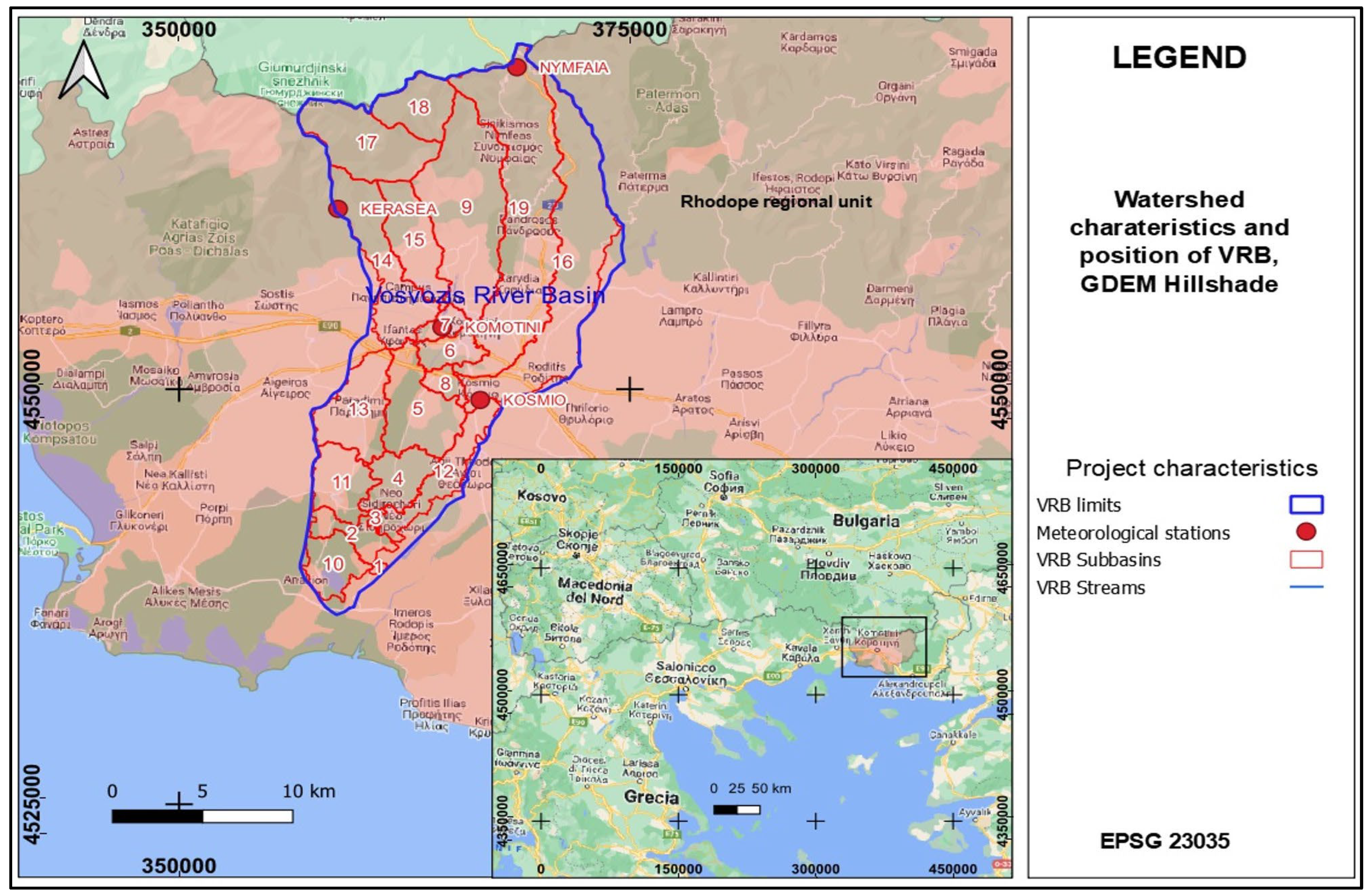
2.1. Study Area Description

VRB with coordinates X = 365,867, Y = 4,555,338 in ED50/UTM zone 35N Coordinate Reference System (EPSG:23035), covers an area of approximately 355 km² in NE Greece, within Thrace region (Figure 1). The length of Vosvozis River course is approximately 40 km, originating from Rhodope mountains and discharging into Ismarida Lake, which is a very important wetland ecosystem protected by the Ramsar treaty on wetlands [38,39,40]. VRB has a diverse topography with a northern mountainous part reaching an altitude of ~1100 m (above sea level-asl) and a southern plain area (with altitudes ranging from 10 to 150 m, where most human activities take place. Agricultural activities are found in the plain part, with cultivation mainly being wheat, cotton, and tobacco. The mountain part is covered by forest of mixed type. The population of the basin area comprises 70,000 inhabitants, while the main urban center is Komotini town, located in the center of the study basin. From the hydrological point of view, VRB forms a typical mountain front recharge system [40], where river flow from the mountain areas provides recharge to the aquifer within the agricultural plain, thus sustaining the farm production in the area, but also the domestic water supply for the urban center of Komotini and the surrounding villages. The climate of the area is Mediterranean, with mild and humid winters (December to February) and hot, dry summers (June to August).

2.2. The SWAT Model

SWAT is a river basin-scale model developed by the USDA Agricultural Research Service (ARS). It is primarily used to estimate the long-term impacts of land management practices on surface water, sediment, and pesticide yields in large watersheds. SWAT is a semi-distributed model that requires inputs such as weather, soil properties, topography, vegetation, and land cover changes that occur in the watershed. In the modeling process, the basin is divided into a series of subbasins, which in turn are divided into hydrological response units (HRUs) [41]. The main model components include hydrology, weather, plant growth, soil temperature, pesticides, nutrients as well as land management [19]. The land phase of the hydrologic cycle is based on the water balance equation (Equation (1)) [41]:

$$S{W}_t=S{W}_0+{{\displaystyle \sum }}_{i=1}^t\left(R_{day}-Q_{surf}-E_a-W_{seep}-Q_{qw}\right)$$

(1)

where $S{W}_t$ is soil water content (final state) (mm); $S{W}_0$ is soil water content (initial state) (mm); $t$ is time (days); $R_{day}$ is the precipitation amounts per day (mm); $Q_{surf}$ is the surface runoff amounts per day $i$ (mm); $E_a$ is the evapotranspiration amounts per day $i$ (mm); $W_{seep}$ is the percolation amount and bypass flow that exit past the bottom of the soil layers per day $i$ (mm); $Q_{qw}$ is the return flow amount per day $i$ (mm).

SWAT model development and the whole procedure are presented in Figure 2.

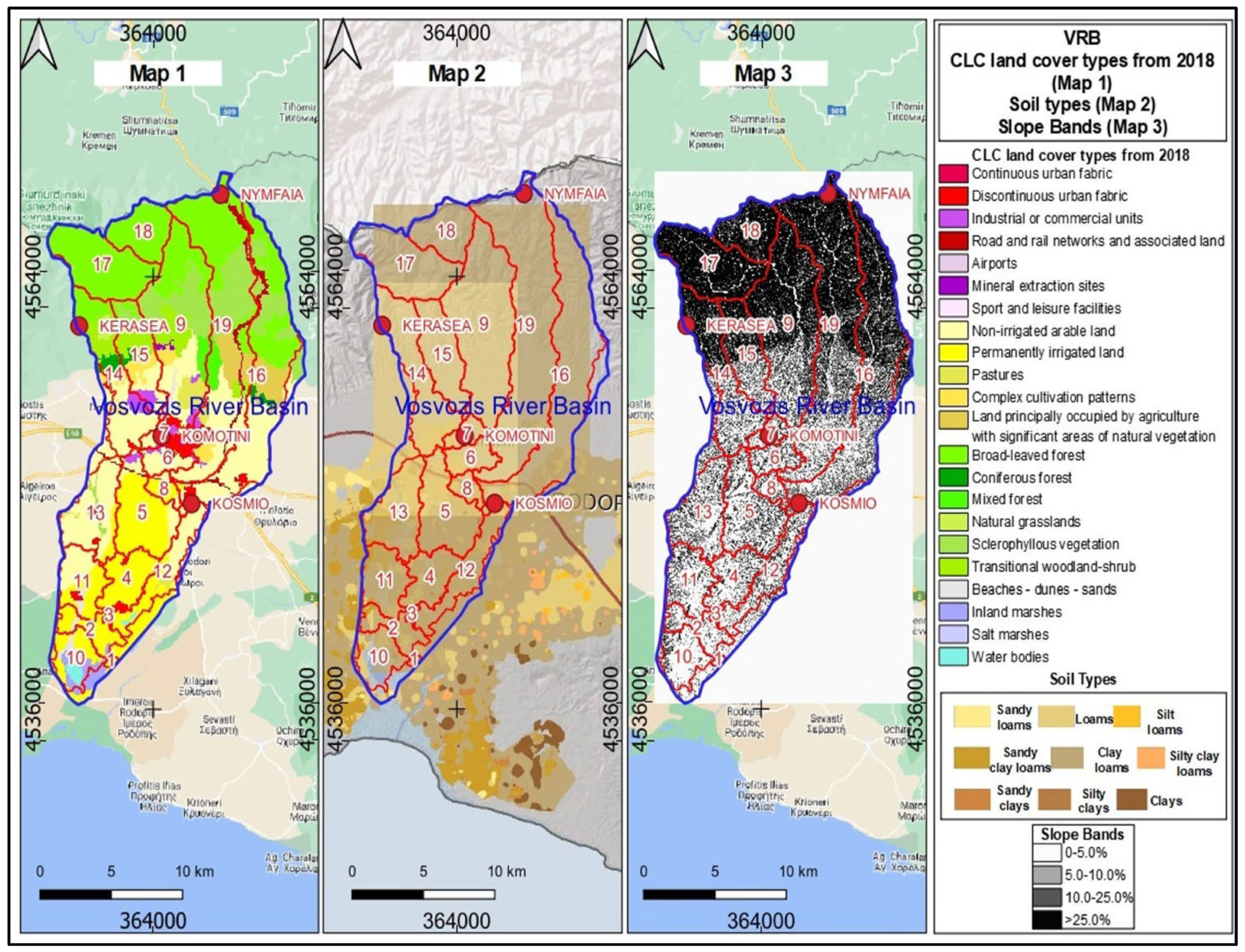
2.3. SWAT Input Data

Simulation of VRB with SWAT requires topography information, which was provided by the ASTER GDEM V3 [42], with a 30 m spatial resolution (Figure 1). The VRB was discretized by the SWAT model into nineteen (19) subbasins as is shown in Figure 1.

CORINE land cover (CLC) was used in order to describe the various land cover types in the study area (Figure 3). CORINE is a pan-European land cover database providing information on 44 land cover types at 100 m spatial resolution (Figure 3) [43]. Therefore, GDEM [44], soil maps, land use maps, and meteorological data were inserted in the SWAT for long-term simulation. On the other hand, in the calibration process with the SWAT-CUP software, the observed discharge values were provided at the VRB catchment outlet.

Soil information for the study basin was accessed from the Food and Agriculture Organization (FAO) at scale of 1:5,000,000 [45]. In order to have a better representation of the soil properties in the study basin the FAO soil map was enhanced with soil data from the 1:500,000 map of Greece [46]. The study area was thus divided into several polygons, each of them containing a hydrologic group of soils, hydraulic conductivity, soil texture, and other chemical and physical properties that are consistent with the FAO soil database (Figure 3).

After providing topography, land cover, and soil information, Vosvozis watershed was divided into 19 subbasins and 101 HRUs based on the classification of land use, soils, and slope presented in Figure 3.

Weather data in the form of minimum and maximum daily temperature and daily precipitation were introduced in SWAT for the time period from 2014 to 2022. Four weather stations operating inside or near the study basin, shown in Figure 1, provided the weather input. Daily precipitation, as well as minimum and maximum daily temperature measurements derived from the above weather stations, are presented in Figure 4, Figure 5 and Figure 6, respectively. Moreover, statistical parameters of collected daily precipitation and minimum and maximum daily temperature, i.e., average, maximum, minimum, and standard deviation (STDEV) are found in

Table 1. Statistical parameters of collected data from meteorological/weather stations in VRB.

ID	NAME	Daily Precipitation (mm)	Daily Maximum Temperature (°C)	Daily Minimum Temperature (°C)
1	KOMOTINI WEATHER STATION	Average: 1.81 Maximum: 121.00 Minimum: 0.00 STDEV: 7.15	Average: 20.39 Maximum: 39.60 Minimum: −5.60 STDEV: 8.81	Average: 8.58 Maximum: 26.10 Minimum: −12.20 STDEV: 7.75
2	NYMFAIA WEATHER STATION	Average: 2.19 Maximum: 82.60 Minimum: 0.00 STDEV: 7.31	Average: 18.66 Maximum: 35.70 Minimum: −4.50 STDEV: 8.93	Average: 7.73 Maximum: 24.85 Minimum: −14.00 STDEV: 7.82
3	KERASEA WEATHER STATION	Average: 2.19 Maximum: 89.60 Minimum: 0.00 STDEV: 6.93	Average: 19.82 Maximum: 37.00 Minimum: −3.30 STDEV: 8.80	Average: 7.56 Maximum: 24.50 Minimum: −12.30 STDEV: 7.82
4	KOSMIO WEATHER STATION	Average: 2.14 Maximum: 91.40 Minimum: 0.00 STDEV: 7.57	Average: 20.85 Maximum: 40.40 Minimum: −3.40 STDEV: 8.69	Average: 7.92 Maximum: 26.40 Minimum: −13.20 STDEV: 7.87

.

SM sensors are operating in three locations in the study basin, namely Kerasea, Komotini, and Nymfaia, providing SM measurements at 10 min intervals at a depth of 5 cm (

Table 2. Characteristics of meteorological and hydrological stations.

ID	Name	Elevation (m)	Measurement Period	SM Measurement Period
1	Komotini Weather Station	33	1 January 2014–31 December 2022	1 January 2019–31 December 2022
2	Nymfaia Weather Station	616	1 January 2019–31 December 2022	1 January 2019–31 December 2022
3	Kerasea Weather Station	587	1 January 2019–31 December 2022	1 January 2019–31 December 2022
4	Kosmio Weather StatioN	60	1 January 2019–31 December 2022	-
5	Vrb Outlet River Gauge	6	1 January 2019–31 December 2022	-

). The present study utilized daily averages of SM from aforementioned sensors to facilitate the verification of the provided Soil Water (SW) parameter obtained from SWAT software. Furthermore, the calibration and verification process for the SWAT model involved assimilation of daily downscaled SM data derived from SMAP mission.

Flow measurements at the outlet point of VRB are conducted from 2019, with a Sommer RQ-30 radar sensor, obtaining 15 min river discharge measurements, as it is shown in Table 2. Daily averages were computed and used in the calibration and validation process.

2.4. Downscaled SMAP SM Retrievals

The SMAP mission developed by NASA, performs remotely sensed global measurements of SM levels within the Earth’s terrestrial regions. SMAP mission differentiates between frozen and thawed land surfaces. The utilization of space-based direct observations to monitor SM and freeze/thaw state results in a noteworthy advancement in the precision of estimates of water, energy, and carbon transfers between the land and the atmosphere. Furthermore, the SMAP initiative employs the aforementioned observations in conjunction with sophisticated modeling and data assimilation techniques to ascertain more profound assessments of root zone SM and net ecosystem exchange of carbon [47]. SM measurements have direct relevance to the evaluation of flood susceptibility and the monitoring of drought conditions. Thus, the utilization of SMAP observations has the potential to aid in the monitoring of various natural hazards, thereby leading to significant economic and social advantages. To assimilate SM information in the SWAT model, we retrieved the recently released downscaled SMAP daily SM at 1 km spatial resolution [48], from [49], available from 1 April 2015 to 29 September 2022. The downscaled SM product is based on the enhanced Level 2 half orbit 9 km SM version 4 product (SPL2SMP_E) available at [50]. The SMAP SM product represents the surface SM conditions, i.e., topsoil layer of 0–5 cm and its accuracy meets the requirement with the vegetation water content ≤ 5 kg/m² [48]. For each subbasin of the study area, the spatial average of daily downscaled SMAP SM was computed. Since the downscaled SM product is available only until September 2022, we used the original SMAP product from 30 September 2022 until 31 December 2022.

In order to approximate SM for the SWAT soil profile of 1 m, the SMAP SM was multiplied to obtain the water equivalent in mm for the predefined soil depth, assuming that it is representative of the moisture conditions for the whole soil profile.

2.5. Calibration with SWAT-CUP Software

SWAT-CUP is a software that analyzes the uncertainty in the estimated output of SWAT software through various calibrations and validations [51,52]. Moreover, the SWAT-CUP is used to study and analyze the SWAT model results, while it helps with testing and adjusting the model, checking its accuracy comparing model results to measurements, and evaluating model uncertainty [53]. The Sequential Uncertainties Fitting Ver-2 (SUFI2) algorithm provided by SWAT-CUP software was used in the calibration procedure; in SUFI2 parameter uncertainty is defined as an interval (uniform distribution) and theoretical models are calculated for multiple sources of uncertainty including parameters, driving factors (e.g., rainfall) and calculated data [51]. Factor uncertainty in model outputs (expressed as a 95% probability distribution) arises as a consequence of increasing numerical precision.

Two static measures are provided in SUFI-2: the R factor and the P factor, which are provided to determine the similarity between simulated and observed results [51]. Moreover, SUFI-2 P factor and R factor static measures are used in order to check how dependable the model predictions are on streamflow, sediment, and nutrient load [54]. The P factor refers to the proportion of observed empirical data encompassed within the confines of a 95% predictive uncertainty (95 PPU) range. One additional measure of static performance is the R factor, which quantifies the average thickness of the 95 PPU zone relative to the standard deviation of observed data. The R factor assumes values from 0 to infinity, while the P factor ranges from 0 to 100%. In order to achieve an optimal simulation that exhibits ideal conformity with empirical observations, the R factor should attain a value of zero while simultaneously producing a P factor equal to unity.

The VRB simulations confirmed the model’s performance with two SWAT-CUP objective functions. The Nash–Sutcliffe [55] and the coefficient of determination R² are the most used objective functions in the calibration process and moreover, they operate effectively even in poor hydrological models [56].

Regarding the calibration of SWAT in VRB, the SWAT model was run from 1 January 2014 to 31 December 2022. The simulation was conducted using a 5-year warm-up period. The calibration period was set for a 2-year period, i.e., from 1 January 2019 to 31 December 2020 while the validation also comprised a 2-year period, from 1 January 2021 to 31 December 2022. A three-fold calibration approach was developed. Initially, the model was calibrated for river gauge measurements, then it was calibrated for satellite-derived SM datasets, and a final calibration attempt used both river gauge and satellite-derived SM datasets in parallel.

3. Results

3.1. Model Calibration and Validation Using River Flow Measurements

River flow measurements help scientists discover climatic or environmental changes because discharge is a function of many parameters such as climate, geology, and topography, which influence synergistically the hydrology of a basin [57], along with soil and land cover types. In this step, model calibration and validation processes were performed at the RCH level with observed river flow measurements at the outlet point of VRB.

To verify model results and quantify the impact of changes in model parameters on model performance, an uncertainty analysis is conducted within SWAT-CUP. In the current study, parameter uncertainty bands for runoff simulations were constructed to represent runoff dynamics in watersheds. First, SWAT was run with different parameter combinations using SWAT-CUP software. Then, the parameters with the best model efficiency (NS > 0.5) were selected from SWAT-CUP (

Table 3. Sensitive parameters used for model calibration with flow measurements. (V means replace and R means relative change).

No	Parameter Name	Parameter Description	Initial Parameter Range
1	R__CN2.mgt	Runoff curve number	(−0.25, 0.25)
2	V__ALPHA_BF.gw	Alpha baseflow factor	(0.01, 1.00)
3	V__GW_DELAY.gw	Groundwater delay time	(0.50, 50.00)
4	V__GWQMN.gw	Threshold water depth in the shallow aquifer required for return flow to occur	(0.01, 5000.00)
5	V__ESCO.hru	Soil evaporation compensation coefficient	(0.01, 1.00)
6	V__EPCO.hru	Plant uptake compensation coefficient	(0.01, 1.00)
7	V__REVAPMN.gw	Reevaporation threshold	(0.01, 500.00)
8	V__GW_REVAP.gw	Groundwater “revap” coefficient	(0.01, 0.20)
9	R__OV_N.hru	Manning’s “n” value for overland flow	(−0.20, 0.20)
10	R__SOL_K(..).sol	Saturated hydraulic conductivity	(−0.15, 0.15)
11	R__SOL_BD(..).sol	Moist bulk density	(−0.15, 0.15)
12	R__SOL_AWC(..).sol	Available water capacity of the soil layer	(−0.15, 0.15)
13	V__CH_BED_BD.rte	Bulk density of channel bed sediment	(1.20, 1.70)
14	V__CH_BNK_BD.rte	Bulk density of channel bank sediment	(1.20, 1.70)
15	V__SURLAG.bsn	Surface runoff lag coefficient	(0.50, 20.00)

). SWAT was run for these parameter sets and simulated runoff data corresponding to each parameter set were extracted. Statistical and graphical displays were utilized to assess the parameter instability bands for the four weather stations in the basin. The number of simulations in the SWAT-CUP software was set to 1000.

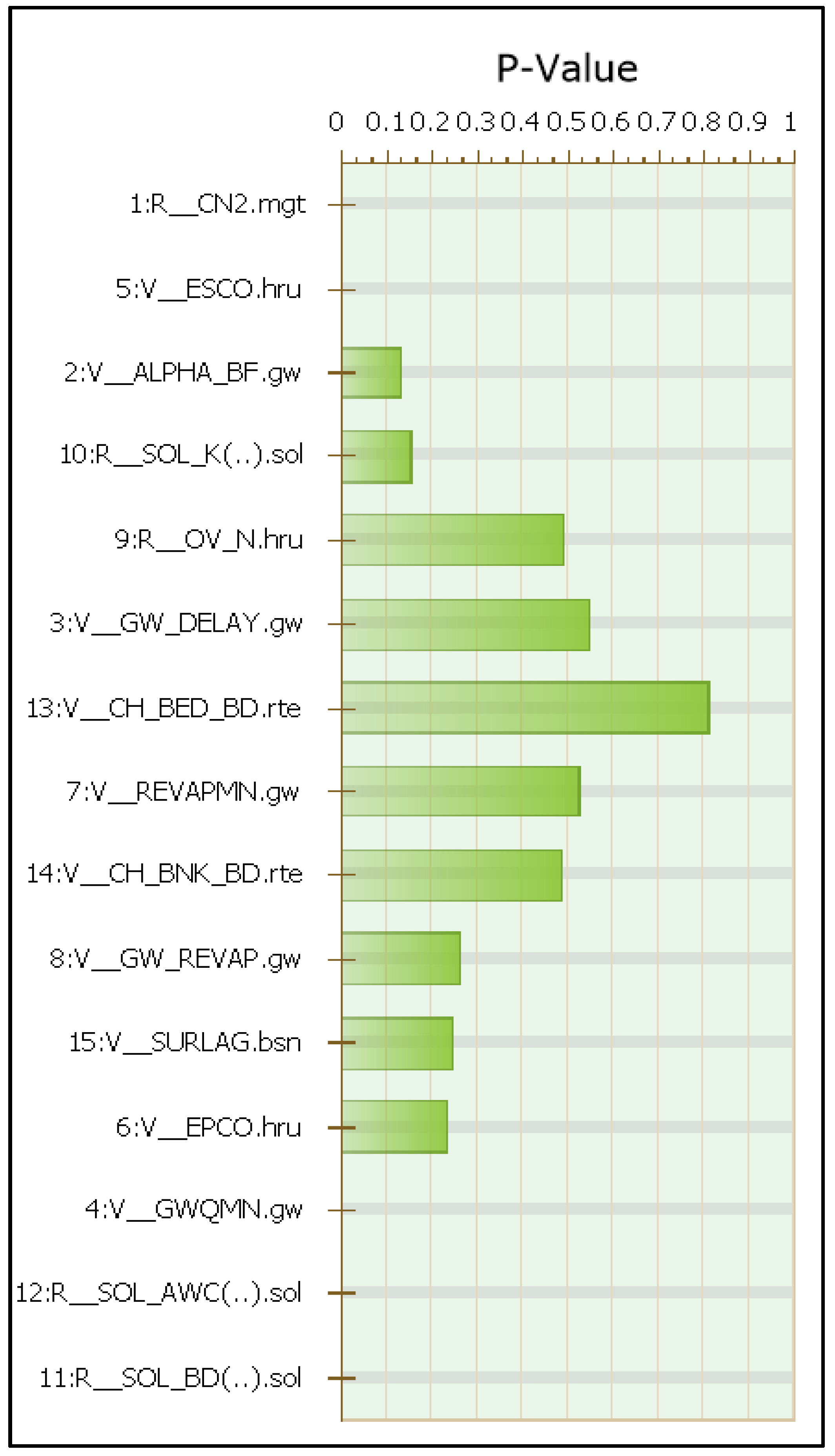
3.1.1. Sensitivity Analysis

In order to calibrate the SWAT model, a total of fifteen parameters that were deemed sensitive were carefully selected. The aforementioned selection was predicated upon the most frequent parameters employed in a total of 64 watershed studies, comprising CN2, ALPHA_BF, GW_DELAY, GWQMN, SOL_AWC, SOL_K, ESCO, EPCO, SURLAG, and OV_N. [58]. Moreover, according to [59], there are initial ranges and other definitions and explanations of the parameters used for model calibration in the study watersheds of their work. Consequently, the SWAT parameters selected for calibrating the VRB SWAT model were employed in a sensitivity analysis conducted via SWAT-CUP on a daily temporal resolution, relative to the VRB’s discharge quantities. The evaluation of sensitivity analysis employed t-statistics and p-values to perform a statistical assessment of the influence of the parameters on the SWAT runoff. The statistical analysis of the t-stat and p-value reveals that the runoff curve number (CN2), the soil evaporation compensation coefficient (ESCO), the threshold water depth in the shallow aquifer required for return flow to occur (GWQMN), the available water capacity of the soil layer (SOL_AWC), and the moist bulk density (SOL_BD) are the most sensitive parameters for VRB as is shown in Figure 7.

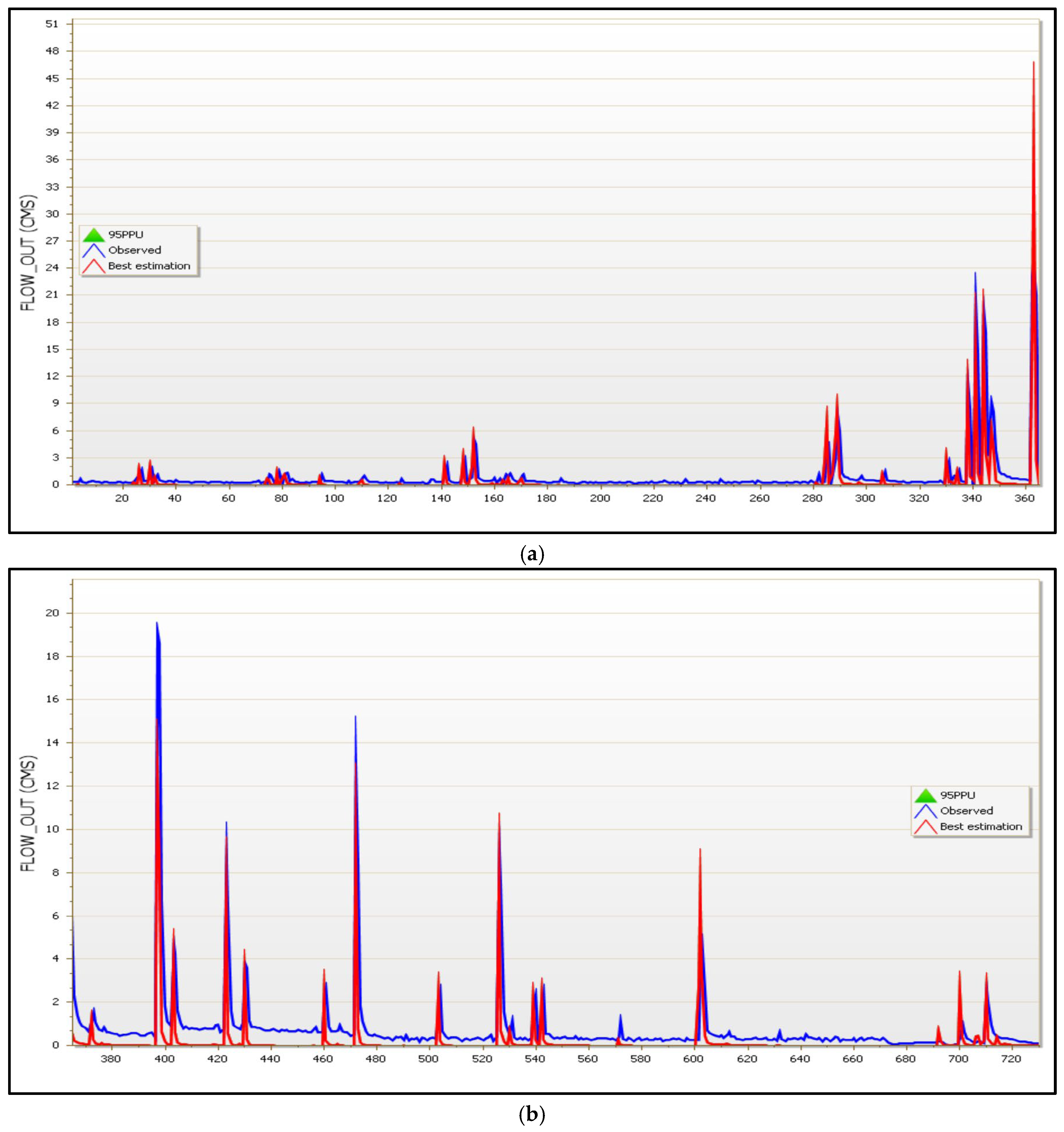
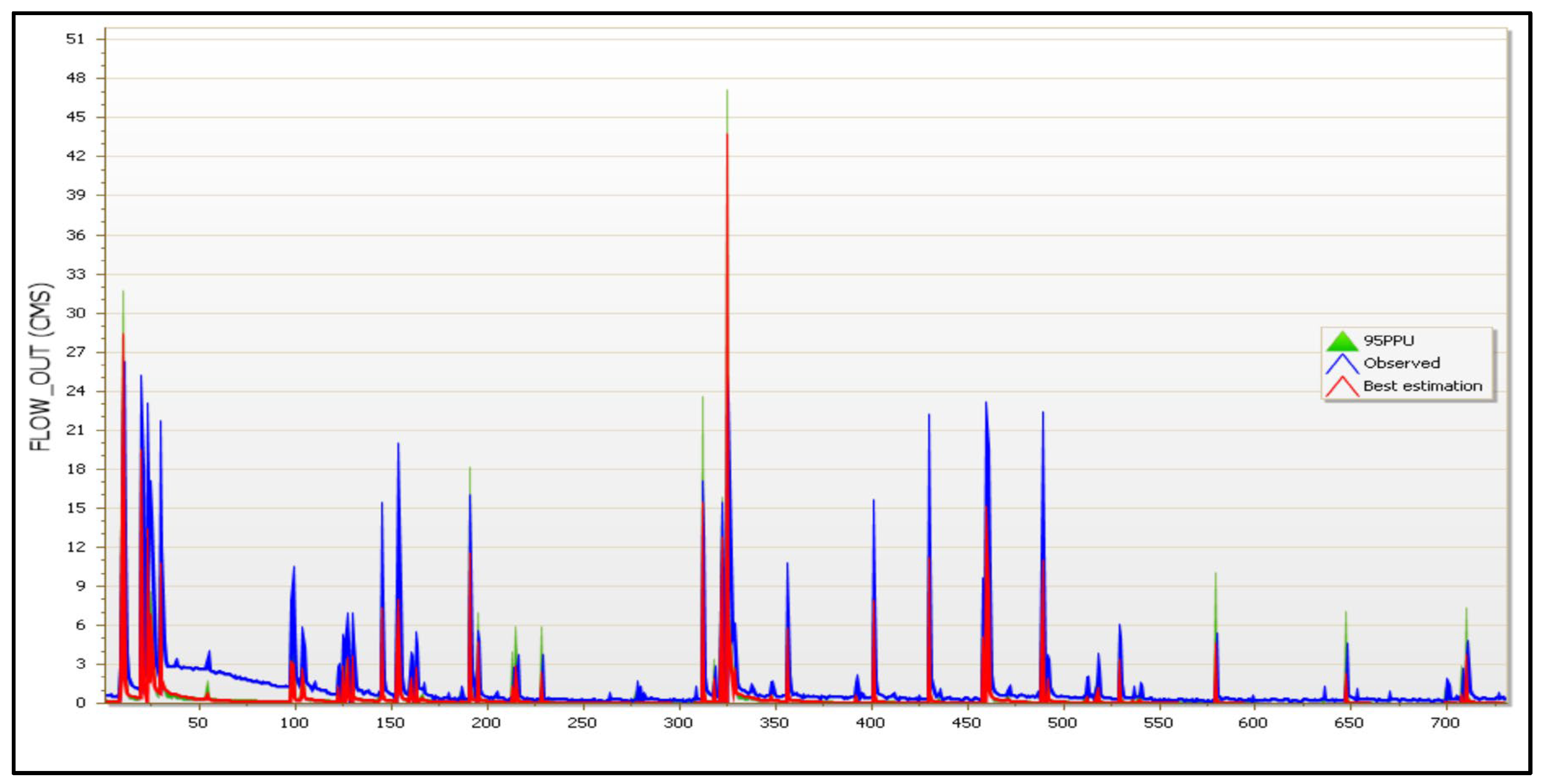
3.1.2. Calibration and Validation Results with Flow Measurements

The calibration of SWAT incorporated all previously indicated sensitive parameters. The model was calibrated at the outlet of reach 1 and at the subbasin 1, where Vosvozis River gauge measurements were taken. In order for the SWAT-CUP process to produce results that are closer to the observed data, calibration and parameter correction work is required.

Table 4. Criteria utilized to determine the precision of model calibration and validation with flow parameters for VRB.

Model Evaluation	R2	NS
CALIBRATION PERIOD (2019–2020)	0.69	0.61
VALIDATION PERIOD (2021–2022)	0.65	0.58

shows R² and NS values results for the time series. Table 4 indicates that the results of the model are satisfactory. This fact can be conducted from the NS coefficient, which is equal to 0.61 and from the R² equal to 0.69 for the calibration procedure, while the NS coefficient is 0.58 and R² is 0.65 for the validation procedure, respectively. Figure 8a,b shows the best simulation against the observed time series of flow and the plot of the 95PPU diagram of all variables for calibration years of the model and is divided into (a) and (b) for calibration years 2019 and 2020, respectively, in order to have a better visualization because of the long daily flow time series. Accordingly, Figure 9a,b shows the best simulation against the observed time series of flow for validation years of the model and is divided into (a) and (b) for validation years 2021 and 2022, respectively.

As mentioned in Section 2.3, SM sensors operate in three locations within VRB limits, namely Kerasea, Komotini, and Nymfaia, and provide SM measurements at 10 min intervals at a depth of 5 cm. In order to check the correctness of daily averages of SW obtained from the SWAT model in the VRB project, they were compared against daily averaged SM measurements obtained from the above 3 SM sensors for the year 2022 (Figure 10). Results showed that while river flow simulation is satisfactory, the SWAT model demonstrated low performance regarding SM (NS = 0.40 and R² = 0.51). It thus seems that the description of the SM regime should be improved.

3.2. Model Calibration and Validation Using SMAP Datasets

SM information plays an important role in hydrologic modeling and environmental protection processes. Recent advances in SM acquisition through remote sensing satellite measurements have attracted attention as an alternative to traditional ground-based SM measurement methods [60]. In the present study, calibration and validation were achieved at the subbasin level with satellite-based derived downscaled SM dataset from the SMAP mission as described in Section 2.4. The number of simulations conducted in the SWAT-CUP software was 1000.

Table 5. Sensitive parameters used for model calibration with SM measurements. (V means replace and R means relative change).

No	Parameter Name	Parameter Description	Initial Parameter Range
1	R__CN2.mgt	Runoff curve number	(−0.25, 0.25)
2	V__ALPHA_BF.gw	Alpha baseflow factor	(0.01, 1.00)
3	V__GW_DELAY.gw	Groundwater delay time	(0.50, 50.00)
4	V__RCHRG_DP.gw	Recharge to deep aquifer	(0.10, 0.50)
5	R__SOL_AWC(..).sol	Available water capacity of the soil layer	(−0.15, 0.15)
6	R__SOL_K(..).sol	Saturated hydraulic conductivity	(−0.15, 0.15)
7	V__ESCO.hru	Soil evaporation compensation coefficient	(0.01, 1.00)
8	V__GW_REVAP.gw	Groundwater “revap” coefficient	(0.01, 0.20)

shows the range of parameters that provided the best model efficiency (NS > 0.5) and therefore were selected for the calibration of satellite-derived SM.

3.2.1. Sensitivity Analysis

To undertake calibration and validation with satellite-derived SM measurements, a set of eight parameters with high sensitivity were selected to be integrated into our model. Subsequently, the parameters of the SWAT-CUP model that were chosen for the calibration and validation of VRB were utilized in a sensitivity analysis of the assimilation of satellite-based SM data from the SMAP mission. The t-stat and p-value results show that the soil evaporation compensation coefficient (ESCO) and the available water capacity of the soil layer (SOL_AWC) are the most sensitive parameters for VRB as shown in Figure 11.

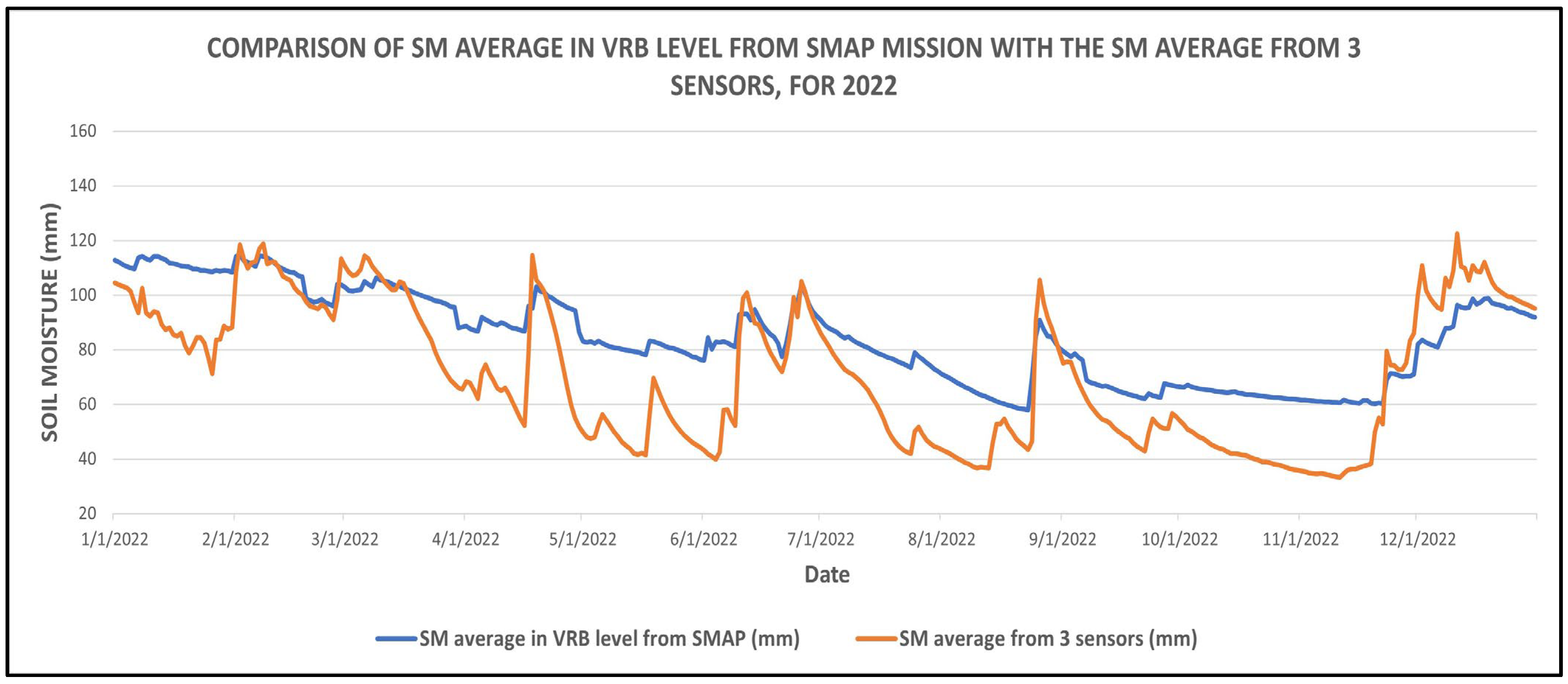
3.2.2. Calibration and Validation Results with SMAP Dataset

The calibration process of SWAT-CUP encompasses the careful inclusion and assessment of all pertinent sensitive parameters. The model was calibrated at the subbasin level. The process of calibration and parameter correction is deemed essential to attenuate the divergence of SWAT-CUP outcomes from the empirically collected data.

Table 6. Criteria utilized to determine the precision of model calibration and validation for satellite-derived SM parameters as they resulted from 19 subbasins average existing in VRB.

Model Evaluation	R2	NS
CALIBRATION PERIOD (2019–2020)	0.66	0.55
VALIDATION PERIOD (2021–2022)	0.58	0.53

depicts the average values of R² and NS metrics for the time series resulting from the 19 subbasins existing in the VRB. Based on the findings elucidated in Table 6, it is deducible that the model demonstrates acceptable performance, as evidenced by the NS coefficient of 0.55 and R² of 0.66 for the calibration procedure and NS coefficient of 0.53 and R² of 0.58 for the validation procedure, respectively. Figure 12 shows the best simulation against satellite-derived subbasin averaged SM values for calibration years, while Figure 13 shows the best simulation against satellite-derived subbasin averaged SM values for validation years of the model. At this point, it is worth mentioning that Figure 12 and Figure 13 refer to subbasin No. 8, which is positioned approximately in the middle of the VRB as depicted in Figure 1. Calibration results namely observed vs. simulated SM, with SMAP mission SM measurements of all the 19 subbasins are included in Supplementary Material S1.

The SM regime seems to be improved this time, while lower performance is observed for the validation period. There are periods of model underestimation of SM, although the general trend of SM seems to be depicted. In this case, we evaluated performance metrics for flow simulation from 2019 to 2022, and it was found that NS = 0.51 and R² = 0.58, which are lower compared to the previous calibration case (Section 3.1), but still satisfactory. Therefore, the model is improved in terms of satellite-based SM simulation, and at the same time the satisfactory performance of river flow is preserved, but still, there is much potential for improvement.

3.3. Model Calibration and Validation Using River Flow and SMAP Datasets

In this final step, we used both flow and satellite-based SM datasets in the calibration procedure, in order to evaluate whether simultaneous calibration using two parameters could possibly improve the model performance for both the examined parameters. Flow calibration and validation were performed at the RCH level while SM calibration and validation were performed at the subbasin level. Observed flow from the four meteorological stations and downscaled SMAP SM were used simultaneously this time. The combination of the two parameters using SWAT-CUP software indicated better calibration results on satellite-derived SM parameters than by using only satellite-based SM parameters in SWAT-CUP software, such as NS equal to 0.85 > 0.55. Moreover, the simulated flow was maintained simultaneously at a satisfactory level with a slight decrease in NS which is equal to 0.57 < 0.61.

The SWAT-CUP program was run with various combinations of parameters. Then, the parameters with the best model efficiency (NS > 0.50) were selected from the SWAT-CUP (

Table 7. Sensitive parameters were used for model calibration with flow and SM measurements. (V means replace and R means relative change).

No	Parameter Name	Parameter Description	Initial Parameter Range
1	R__CN2.mgt	Runoff curve number	(−0.25, 0.25)
2	V__ALPHA_BF.gw	Alpha baseflow factor	(0.01, 1.00)
3	V__GW_DELAY.gw	Groundwater delay time	(0.50, 50.00)
4	V__GWQMN.gw	Threshold water depth in the shallow aquifer required for return flow to occur	(0.01, 5000.00)
5	V__ESCO.hru	Soil evaporation compensation coefficient	(0.01, 1.00)
6	V__EPCO.hru	Plant uptake compensation coefficient	(0.01, 1.00)
7	V__REVAPMN.gw	Reevaporation threshold	(0.01, 500.00)
8	V__GW_REVAP.gw	Groundwater “revap” coefficient	(0.01, 0.20)
9	R__OV_N.hru	Manning’s “n” value for overland flow	(−0.20, 0.20)
10	R__SOL_K(..).sol	Saturated hydraulic conductivity	(−0.15, 0.15)
11	R__SOL_BD(..).sol	Moist bulk density	(−0.15, 0.15)
12	R__SOL_AWC(..).sol	Available water capacity of the soil layer	(−0.15, 0.15)
13	V__CH_BED_BD.rte	Bulk density of channel bed sediment	(1.20, 1.70)
14	V__CH_BNK_BD.rte	Bulk density of channel bank sediment	(1.20, 1.70)
15	V__SURLAG.bsn	Surface runoff lag coefficient	(0.50, 20.00)
16	V__RCHRG_DP.gw	Recharge to deep aquifer	(0.10, 0.50)

). Finally, SWAT-CUP was run with this parameter set, and the simulated flow rates and SM data corresponding to each parameter set were extracted. Both statistical measures and graphs were used to estimate parameter uncertainty bands for the four meteorological stations in the watershed. The simulations performed in the SWAT-CUP calibration process were 1000.

3.3.1. Sensitivity Analysis

A total of sixteen parameters of sensitivity were designated for the purpose of calibrating and validating our model. Consequently, the SWAT flow and SM parameters employed for the third calibration and validation attempt were subjected to a sensitivity analysis, considering daily time intervals, based on the recorded flow obtained from the river gauge measurements and downscaled satellite-derived SM measurements obtained from the SMAP mission. Sensitivity analyses were conducted utilizing both t-statistics and p-values to statistically assess the impact of the aforementioned parameters on the hydrologic and SM parameters of the SWAT. The statistical outputs indicated that the t-stat and p-value provide evidence that the available water capacity of the soil layer (SOL_AWC), the runoff curve number (CN2), and the groundwater delay time (GW_DELAY) are the most sensitive parameters for VRB as shown in Figure 14.

3.3.2. Calibration and Validation Results with River Flow and SMAP Dataset

In SWAT calibration, all sensitive parameters are taken into account; a process of calibration and parameter correction is necessary for SWAT-CUP to estimate the most appropriate model parameters and obtain results closer to the observed data.

Table 8. Criteria utilized to determine the precision of model calibration and validation with flow and satellite-derived SM parameters as they resulted from 19 subbasins average existing in VRB.

Model Evaluation	R2	NS
CALIBRATION PERIOD FOR FLOW PARAMETER (2019–2020)	0.66	0.57
VALIDATION PERIOD FOR FLOW PARAMETER (2021–2022)	0.64	0.54
CALIBRATION PERIOD FOR SM PARAMETER (2019–2020)	0.91	0.85
VALIDATION PERIOD FOR SM PARAMETER (2021–2022)	0.84	0.79

shows the results of R² and NS values in the time series. From Table 8, it can be concluded that the model results are satisfactory for the calibration and validation procedure for the flow parameters with NS coefficients of 0.57, R² = 0.66, NS coefficient 0.54, and R² = 0.64 for the calibration and validation phase, respectively. Moreover, Table 8 shows the performance metrics averaged over the 19 subbasins, indicating the NS coefficient equal to 0.85 and R² equal to 0.91, and the NS coefficient equal to 0.79 and R² equal to 0.84 for the calibration and validation procedures of the SM parameter, respectively. Figure 15 shows the best simulation against the observed time series of flow parameters and the plot of the 95PPU diagram of all variables for the calibration years of the model, while Figure 16 shows the best simulation against the observed time series of flow parameters for validation years of the model. Moreover, Figure 17 shows the best simulation against the observed time series of the SM parameter and the plot of the 95PPU diagram of all variables for calibration years of the model and Figure 18 shows the best simulation against the observed time series of the SM parameter for the validation years of the model. Specifically, Figure 17 and Figure 18 refer to subbasin No. 8, while the corresponding observed and simulated results of the calibration procedure of all the 19 subbasins are given as Supplementary Material S2.

To check whether the SWAT model captures the temporal variability of SM at the basin level, we compared the basin-averaged daily SWAT SM against the average SM of the three ground sensors for 2022, assuming that they represent the average SM conditions in the study basin, as they cover a wide part of the basin. Comparing Figure 8 (SWAT calibration with flow measurements only) and Figure 19 (SWAT simultaneous calibration with flow and SM), it can be concluded that the representation of the average SM conditions is improved in the SWAT model after being calibrated simultaneously for flow and SM. The computed NS = 0.73 and R² = 0.81 for SM compared to ground measurements proves this considerable improvement. It can be seen thus that the assimilation of satellite SM can contribute to the enhancement of SM modeling which is of great importance, especially for sparsely gauged basins.

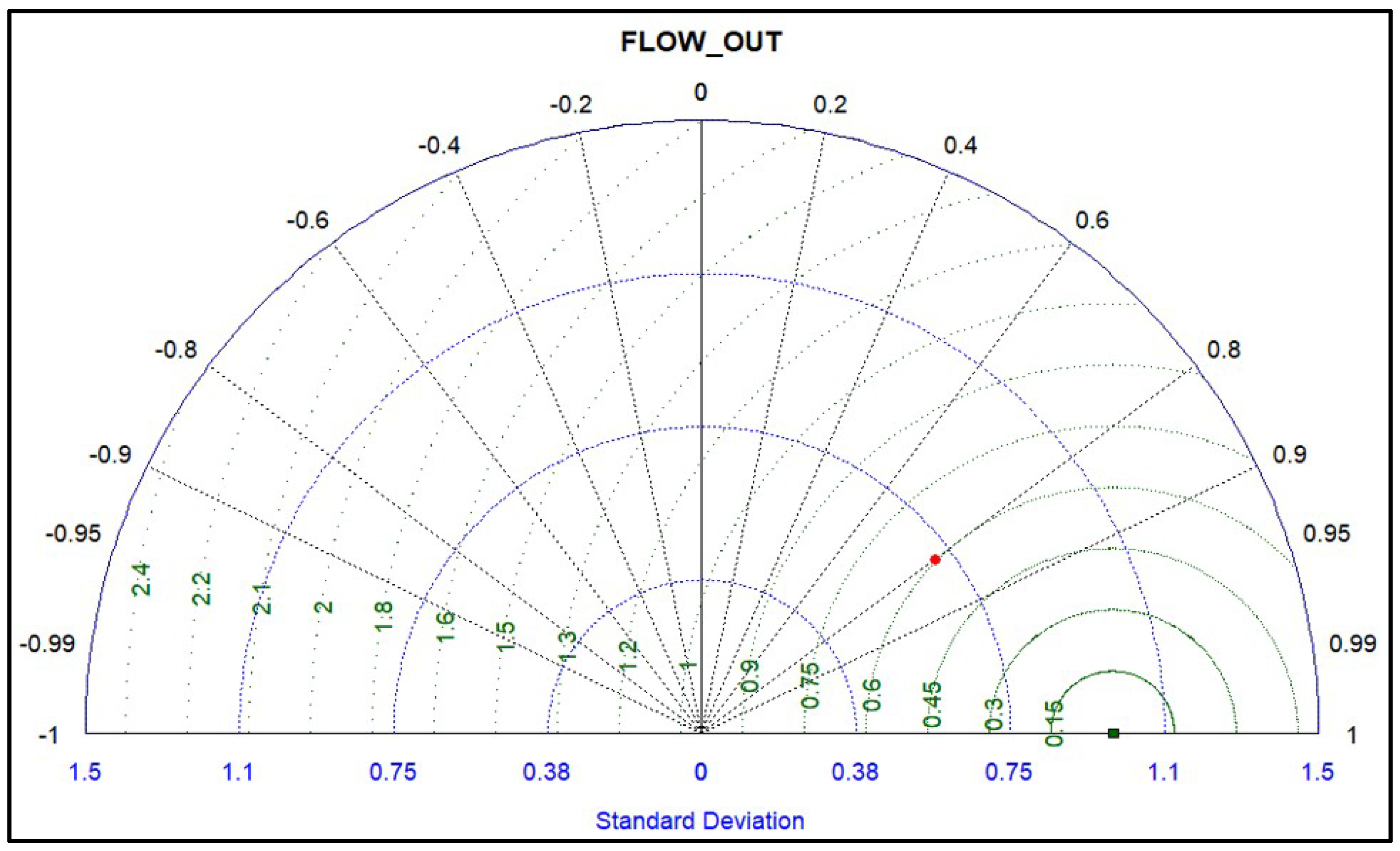
3.3.3. Model Evaluation Performance Indicators

In the third case, where calibration was performed simultaneously using both river flow and SMAP datasets, in order to evaluate the performance of the studied model, NS and R² statistics were used and presented in Table 8. Moreover, two graphic methods, namely Box It can inform us where the middle value is and how spread out the numbers are. It also helps us find any unusual plot and Taylor diagrams that were used in this regard. A box plot is a graphical non-parametric (i.e., there is no assumption of the underlying statistical distribution) representation of samples of numerical data used to show information about the numerical data quartiles and thus identify the skewness, spread, and variability of samples and whether there are outliers in the dataset [61]. The Taylor diagram is a successful strategy for comparative assessment of various models, that shows graphically the important statistical information of models and displays the results of evaluation indicators consistently [62,63]. In this work, we checked the developed model, using the box plot and the Taylor diagram of the flow parameter as shown in Figure 20 and Figure 21, respectively. Figure 20, of the observed daily flow values and the corresponding simulated values, demonstrates a satisfactory estimation of flow as far as median values are concerned. Whereas a lower ability of the model to simulate high river flow values is found, as is also evidenced by Figure 15 and Figure 16. In the Taylor diagram, if a model is close to the reference point (the hollow circle on the horizontal line), it means it is more reliable. As a result, Figure 21 shows that this study model has a short distance to the reference point and as a result, has high performance and accuracy. Moreover, according to Figure 21 (red dot), the correlation between the observed and simulated daily stream flow data is 0.80. Moreover, the box plot and the Taylor diagram of the SMAP SM parameter used in our study model, were drawn in Figure 22 and Figure 23, respectively, and concern subbasin No. 8. Figure 22 of the observed daily SMAP SM values and the corresponding simulated values shows a minor overestimation of the median of the simulated values compared to the observed values. Finally, Figure 23 shows that this study model has a short distance to the reference point and as a result, has high performance and accuracy. Moreover, according to Figure 23 (red dot), the correlation between the observed daily SMAP SM and simulated daily SM is 0.90.

As was mentioned above, Figure 22 and Figure 23 refer to subbasin No. 8., while the corresponding box plots and Taylor diagrams of the remaining 18 subbasins are given as Supplementary Material S3. It is worth mentioning that in Supplementary Material S3, while the Taylor diagrams of the remaining 18 project subbasins are displayed in isolated graphs, the box plots of them are presented in one graph.

3.4. Advantages and Disadvantages of the Proposed Model

The proposed model improves the modeling performance related to soil moisture, which is of major importance related to the prevalence of extreme hydrological conditions, i.e., floods and droughts, but also for crop production. Thus, the calibrated model can be applied even at the field scale in order to acquire information on soil moisture conditions and facilitate irrigation planning. At the catchment scale, the expected advantages of the model are: (1) SM regime may contribute to improved planning of anticipating water resources management measures through SWAT software, which was used in this model and is based on physical principles. (2) Even though SM sensors are scarce, having downscaled SMAP SM measurements may help us predict the effects of several hydrological conditions that have strong environmental impacts. (3) Even though SM and discharge measurement sensors have gaps in time series, by using the weather generator, missing data can be filled when needed. (4) In the proposed model, SWAT-CUP software was used for automatic calibration using auto-calibration and uncertainty algorithm SUFI2 analyzed and improved SM and flow parameters. (5) Through SWAT-CUP software and the multi-objective calibration, better simulation was obtained that matched SM and flow observations by improving the NS and R² values of SM and flow parameters, thus helping to better represent various hydrological processes in the study basin.

Although the model has many advantages, there are also some limitations. Thus, the model uses only the amount of rain that falls in a single day and applies the Soil Conservation Services-CN method to it, thus neglecting rainfall intensity at the sub-daily time step, and the associated flood conditions that may occur at this time scale, although providing moisture conditions antecedent to heavy rainfall events may contribute to the forecasting of flood conditions and up to this point the presented herein approach is helpful. Another issue is the spatial variability of rainfall which cannot be accommodated in data-scarce regions, with a consequent impact on model performance. In the case of the present work, rainfall data availability and the dispersion of rainfall gauge stations in the study basin were sufficient for reliable model development. However, this is not always the case and in large and sparsely gauged basins researchers might have to rely on remotely sensed precipitation as an alternative to account for the spatial variability of rainfall.

3.5. Discussion

Within the present work, three independent calibration/validation exercises using SWAT and SWAT-CUP in VRB were conducted. The calibration period was that of 2019–2020 whereas years 2021–2022 were used as the validation period. In the first two approaches, SWAT was calibrated against a sole parameter, i.e., daily averaged river flow and downscaled daily satellite-derived SM from SMAP mission, respectively. In the third case, SWAT was calibrated simultaneously against both daily averaged flow and SMAP SM parameters. Results indicated a satisfactory performance regarding flow simulation in the first trial (calibration with flow measurements only) with NS = 0.61 and R² = 0.69 for the calibration period, while for the validation period, the results were 0.58 and 0.65, respectively. Sensitivity analysis indicated the runoff curve number, the soil evaporation compensation coefficient, the threshold water depth in the shallow aquifer required for return flow to occur, the available water capacity of the soil layer, and the moist bulk density, as the most sensitive parameters for VRB. The model, however, demonstrated a low predictive ability regarding SM in the study area. The second case, i.e., calibration against SM, resulted in a good performance, although lower compared to the flow calibration case with NS = 0.55 and R² = 0.66 for the calibration period, while for the validation period, the results were 0.53 and 0.58, respectively. The most sensitive parameters were found to be the soil evaporation compensation coefficient and the available water capacity of the soil layer. In the final case, i.e., a multi-objective calibration with simultaneous calibration against SM and river flow resulted in NS = 0.57 and R² = 0.66 and NS = 0.54 and R² = 0.64 for flow calibration and validation period, respectively, while a considerable improvement was achieved for SM at subbasin scale, with NS = 0.85 and R² = 0.91 and NS = 0.79 and R² = 0.84 for the calibration and validation period, respectively. This time, the most important parameters were found to be the available water capacity of the soil layer, the runoff curve number, and the groundwater delay time. Results reveal that SM parameter uncertainty is higher than flow-related uncertainty. Nevertheless, one should keep in mind the inherent differences between satellite-derived SM and the SM acquired by the SWAT model. The former represents surface SM conditions whereas the latter describes the unsaturated zone average moisture conditions, which might be quite different, and a perfect match should not be sought. Verifying results using ground SM observations provides a useful way to examine the model performance in terms of SM description, as is performed in the present work.

In all simulations, the timing of peak flow was successfully depicted; however, the actual peak flow was many times underestimated, indicating that there is a considerable space for improvement, as far as peak flow is concerned, which requires additional locations of discharge measurements, which were not available in the present work, to allow runoff calibration at the subbasin level. Analogous underestimation of river flow was observed in [37], attributed to a lack of data to allow the application of the SWAT reservoir module in hydropower generation-affected subbasins. Nevertheless, lack of hydrological information is a very frequent problem and not many basins have continuous flow measurements in many locations, as it is difficult and costly to install and operate such an observational network. Many basins around the world remain ungauged or have little recorded streamflow information [64,65] and this is the main issue that constrains the development of robust hydrological models. Analogous observations were highlighted in previous works while simulating daily flow [66] but even at the monthly time step [67], attributed mainly to the sparse and heterogeneous spatial distribution of meteorological stations and the associated inaccurate precipitation inputs to SWAT [67], or to inaccurate stream delineation [66].

Regarding the study area’s water budget, the basin annual average values during a long-term period of simulation (including the 5 warm-up years) from 1 January 2014 to 31 December 2022, provided the following results 606.9 mm precipitation, 148.59 mm surface runoff Q, 417.2 mm evaporation and transpiration and 47.99 mm percolation to shallow aquifer.

Compared to previous works, our results are analogous to that of [32] in the Mundaú River Basin (4090.39 km²) in Northeastern Brazil, where authors calibrated against both river gauge and SM data, highlighting the potential for improved model performance assimilating SM information, especially in cases where discharge data are scarce. The advantages of the multi-objective calibration approach that resulted in the improvement of simulation results for other parameters such as snow water equivalent along with realistic river flow predictions is highlighted in previous work [37], indicating that not only soil moisture regime can be described better but also snow water processes, which is a very important hydrological component in snow-dominated basins.

In other studies, however, step-wise calibration against the flow and satellite-based SM measurements performed better compared to simultaneous calibration in the study presented in [1] at the Hydrological Open-Air Laboratory (HOAL) catchment located in Petzenkirchen, Lower Austria. It should be noted, however, that HOAL is a very small catchment of 66 ha, with a dense network of gauge stations, and the SWAT calibration and validation incorporated runoff, groundwater flow, crop yields, and SM data. This is of course the ideal case, which, however, cannot be accommodated in the majority of basins, where data scarcity restricts such applications. In the present work, results from the SWAT-CUP indicated that when SM and flow parameters are used both in order to simultaneously calibrate and validate the model, the results of the simulation process are more satisfactory. This is an important finding, as acquiring SM data is an easily and quickly achievable procedure nowadays when a wealth of satellite observations is readily available, compared to the cost and effort required for continuous river gauge measurements.

Future works extending the present findings can be conducted, related to the assimilation of remotely sensed gridded SM so as to estimate SM at the finer spatial resolution, e.g., at the field scale, which is of particular importance for agricultural activities and the anticipation of flood and drought conditions. Moreover, adding more streamflow gauge stations and SM estimates in specific locations could potentially improve the accuracy of predicting the average and pick streamflow across the watershed and its individual subbasins. However, this is not the usual case as there are important constraints related to the cost and effort of river gauge monitoring networks, mentioned above. Nevertheless, several remotely sensed datasets are freely available nowadays and their usefulness in model development, calibration, and validation has been indicated in previous works [68] and it is believed that they will offer a viable solution for hydrological modeling in sparsely monitored areas. The improved ability to predict and the reduced uncertainty of SWAT simulations using SM parameters, as demonstrated in this study, can greatly help the research on long-term effects of climate change and land use, predicting floods and droughts, as well as managing agricultural practices in order to improve crop yield.

4. Conclusions

Within the present work, QSWAT and SWAT-CUP were used for the simulation of the hydrological components in a catchment in Northeastern Greece. Three calibration and validation approaches were tested, i.e., an initial one calibrating only against river gauge measurements, a second one calibrating only against satellite-derived SM measurements, and a third one calibrating simultaneously against both flow and SM measurements at the daily time step. Results indicated a satisfactory performance in all three cases, for flow conditions, while the third one, using both parameters in a multi-objective calibration, produced the best SM results, while preserving the successful simulation of river flow, as indicated by the performance metrics and the box plots and Taylor diagrams provided. This is especially important since SM is of major importance related to the prevalence of extreme hydrological conditions like floods and drought surges, while a better representation of the SM regime may contribute to improved planning of anticipating measures.

References

1. Musyoka, F.K.; Strauss, P.; Zhao, G.; Srinivasan, R.; Klik, A. Multi-step calibration approach for SWAT model using soil moisture and crop yields in a small agricultural catchment. Water 2021, 13, 2238. [Google Scholar] [CrossRef]
2. Mishra, S.K.; Gajbhiye, S.; Pandey, A. Estimation of design runoff curve numbers for Narmada watersheds (India). J. Appl. Water Eng. Res. 2013, 1, 69–79. [Google Scholar] [CrossRef]
3. Rafiei-Sardooi, E.; Azareh, A.; Choubin, B.; Mosavi, A.H.; Clague, J.J. Evaluating urban flood risk using hybrid method of TOPSIS and machine learning. Int. J. Disaster Risk Reduct. 2021, 66, 102614. [Google Scholar] [CrossRef]
4. Wijayarathne, D.B.; Coulibaly, P. Identification of hydrological models for operational flood forecasting in St. John’s, Newfoundland, Canada. J. Hydrol. Reg. Stud. 2020, 27, 100646. [Google Scholar] [CrossRef]
5. Khan, U.; Ajami, H.; Tuteja, N.K.; Sharma, A.; Kim, S. Catchment scale simulations of soil moisture dynamics using an equivalent cross-section based hydrological modelling approach. J. Hydrol. 2018, 564, 944–966. [Google Scholar] [CrossRef]
6. Ng, H.Y.F.; Marsalek, J. Simulation of the effects of urbanization on basin streamflow. JAWRA J. Am. Water Resour. Assoc. 1989, 25, 117–124. [Google Scholar] [CrossRef]
7. Beven, K. Rainfall-Runoff Modelling; John Wiley & Sons: Hoboken, NJ, USA, 2012; ISBN 9780470714591. [Google Scholar]
8. Devi, G.K.; Ganasri, B.P.; Dwarakish, G.S. A Review on Hydrological Models. Aquat. Procedia 2015, 4, 1001–1007. [Google Scholar] [CrossRef]
9. Abbott, M.B.; Bathurst, J.C.; Cunge, J.A.; O’Connell, P.E.; Rasmussen, J. An introduction to the European Hydrological System—Systeme Hydrologique Europeen,“SHE”, 2: Structure of a physically-based, distributed modelling system. J. Hydrol. 1986, 87, 61–77. [Google Scholar] [CrossRef]
10. Abbott, M.B.; Bathurst, J.C.; Cunge, J.A.; O’Connell, P.E.; Rasmussen, J. An introduction to the European Hydrological System—Systeme Hydrologique Europeen, “SHE”, 1: History and philosophy of a physically-based, distributed modelling system. J. Hydrol. 1986, 87, 45–59. [Google Scholar] [CrossRef]
11. Šimůnek, J.; Van Genuchten, M.T.; Šejna, M. The HYDRUS2D Software Package for Simulating the Two-Dimensional Movement of Water, Heat, and Multiple Solutes in Variably-Saturate Media, Version 2.0; U.S. Department of Agriculture: Riverside, CA, USA, 1999.
12. Šimůnek, J.; Van Genuchten, M.T.; Šejna, M. The HYDRUS-1D Software Package for Simulating the One-Dimensional Movement of Water, Heat, and Multiple Solutes in Variably-Saturated Media, Version 3.0; Department of Environmental Sciences, University of California: Riverside, CA, USA, 2005. [Google Scholar]
13. Šimůnek, J.; Van Genuchten, M.T.; Šejna, M. The HYDRUS Software Package for Simulating the Two- and Three-Dimensions Movement of Water, Heat, and Multiple Solutes in Variably-Saturated Media, Version 1.0; PC Progress: Prague, Czech Republic, 2006. [Google Scholar]
14. Kollet, S.J.; Maxwell, R.M. Integrated surface-groundwater flow modeling: A free-surface overland flow boundary condition in a parallel groundwater flow model. Adv. Water Resour. 2006, 29, 945–958. [Google Scholar] [CrossRef]
15. Flugel, W.-A. Delineating hydrological response units by geographical information system analyses for regional hydrological modelling using prms/mms in the drainage basin of the river brol, germany. Hydrol. Process. 1995, 9, 423–436. [Google Scholar] [CrossRef]
16. Refsgaard, J.C.; Knudsen, J. Operational Validation and Intercomparison of Different Types of Hydrological Models. Water Resour. Res. 1996, 32, 2189–2202. [Google Scholar] [CrossRef]
17. Kirchner, J.W. Getting the right answers for the right reasons: Linking measurements, analyses, and models to advance the science of hydrology. Water Resour. Res. 2006, 42, 1–5. [Google Scholar] [CrossRef]
18. Arnold, J.G.; Srinivasan, R.; Muttiah, R.S.; Williams, J.R. Large area hydrologic modeling and assessment Part I: Model development. J. Am. Water Resour. Assoc. 1998, 34, 73–89. [Google Scholar] [CrossRef]
19. Gassman, P.W.; Reyes, M.R.; Green, C.H.; Arnold, J.G. The Soil and Water Assessment Tool: Historical Development, Applications, and Future Research Directions. Trans. ASABE 2007, 50, 1211–1250. [Google Scholar] [CrossRef]
20. Saleh Al-Khafaji, M.; Saeed, F. Effect of DEM and Land Cover Resolutions on Simulated Runoff of Adhaim Watershed by SWAT Model. Eng. Technol. J. 2018, 36, 439–448. [Google Scholar] [CrossRef]
21. Al-Khafaji, M.S.; Al-Mukhtar, M.; Mohena, A. Performance of SWAT Model for Long-Term Runoff Simulation within Al-Adhaim Watershed, Iraq. Int. J. Sci. Eng. Res. 2017, 8, 1510. [Google Scholar]
22. Farhan, A.M.; Thamiry, D.H.A. Al Estimation of the Surface Runoff Volume of Al-Mohammedi Valley for Long-Term period using SWAT Model. Iraqi J. Civ. Eng. 2020, 14, 7–12. [Google Scholar] [CrossRef]
23. Marek, G.W.; Gowda, P.H.; Evett, S.R.; Baumhardt, R.L.; Brauer, D.K.; Howell, T.A.; Marek, T.H.; Srinivasan, R. Calibration and validation of the SWAT model for predicting daily ET over irrigated crops in the Texas High Plains using lysimetric data. Trans. ASABE 2016, 59, 611–622. [Google Scholar] [CrossRef]
24. Fang, B.; Kansara, P.; Dandridge, C.; Lakshmi, V. Drought monitoring using high spatial resolution soil moisture data over Australia in 2015–2019. J. Hydrol. 2021, 594, 125960. [Google Scholar] [CrossRef]
25. Sungmin, O.; Hou, X.; Orth, R. Observational evidence of wildfire-promoting soil moisture anomalies. Sci. Rep. 2020, 10, 11008. [Google Scholar]
26. Sazib, N.; Bolten, J.D.; Mladenova, I.E. Leveraging NASA Soil Moisture Active Passive for Assessing Fire Susceptibility and Potential Impacts Over Australia and California. IEEE J. Sel. Top. Appl. Earth Obs. Remote Sens. 2022, 15, 779–787. [Google Scholar] [CrossRef]
27. Kumar, S.V.; Dirmeyer, P.A.; Peters-Lidard, C.D.; Bindlish, R.; Bolten, J. Information theoretic evaluation of satellite soil moisture retrievals. Remote Sens. Environ. 2018, 204, 392–400. [Google Scholar] [CrossRef] [PubMed]
28. Ali, M.H.; Popescu, I.; Jonoski, A.; Solomatine, D.P. Remote Sensed and/or Global Datasets for Distributed Hydrological Modelling: A Review. Remote Sens. 2023, 15, 1642. [Google Scholar] [CrossRef]
29. Hashem, A.A.; Engel, B.A.; Marek, G.W.; Moorhead, J.E.; Flanagan, D.C.; Rashad, M.; Radwan, S.; Bralts, V.F.; Gowda, P.H. Evaluation of SWAT Soil Water Estimation Accuracy Using Data from Indiana, Colorado, and Texas. Trans. ASABE 2020, 63, 1827–1843. [Google Scholar] [CrossRef]
30. Uniyal, B.; Dietrich, J.; Vasilakos, C.; Tzoraki, O. Evaluation of SWAT simulated soil moisture at catchment scale by field measurements and Landsat derived indices. Agric. Water Manag. 2017, 193, 55–70. [Google Scholar] [CrossRef]
31. Coopersmith, E.J.; Cosh, M.H.; Petersen, W.A.; Prueger, J.; Niemeier, J.J. Soil Moisture Model Calibration and Validation: An ARS Watershed on the South Fork Iowa River. J. Hydrometeorol. 2015, 16, 1087–1101. [Google Scholar] [CrossRef]
32. De Andrade, C.W.L.; Montenegro, S.M.G.L.; Montenegro, A.A.A.; Lima, J.R.D.S.; Srinivasan, R.; Jones, C.A. Soil moisture and discharge modeling in a representative watershed in northeastern Brazil using SWAT. Ecohydrol. Hydrobiol. 2019, 19, 238–251. [Google Scholar] [CrossRef]
33. Van Der Velde, R.; Colliander, A.; Pezij, M.; Benninga, H.J.F.; Bindlish, R.; Chan, S.K.; Jackson, T.J.; Hendriks, D.M.D.; Augustijn, D.C.M.; Su, Z. Validation of SMAP L2 passive-only soil moisture products using upscaled in situ measurements collected in Twente, the Netherlands. Hydrol. Earth Syst. Sci. 2021, 25, 473–495. [Google Scholar] [CrossRef]
34. Zare, M.; Azam, S.; Sauchyn, D. A Modified SWAT Model to Simulate Soil Water Content and Soil Temperature in Cold Regions: A Case Study of the South Saskatchewan River Basin in Canada. Sustainability 2022, 14, 10804. [Google Scholar] [CrossRef]
35. Pignotti, G.; Crawford, M.; Han, E.; Williams, M.R.; Chaubey, I. SMAP soil moisture data assimilation impacts on water quality and crop yield predictions in watershed modeling. J. Hydrol. 2023, 617, 129122. [Google Scholar] [CrossRef]
36. Eini, M.R.; Massari, C.; Piniewski, M. Satellite-based soil moisture enhances the reliability of agro-hydrological modeling in large transboundary river basins. Sci. Total Environ. 2023, 873, 162396. [Google Scholar] [CrossRef] [PubMed]
37. Tuo, Y.; Marcolini, G.; Disse, M.; Chiogna, G. A multi-objective approach to improve SWAT model calibration in alpine catchments. J. Hydrol. 2018, 559, 347–360. [Google Scholar] [CrossRef]
38. Gemitzi, A.; Stefanopoulos, K. Evaluation of the effects of climate and man intervention on ground waters and their dependent ecosystems using time series analysis. J. Hydrol. 2011, 403, 130–140. [Google Scholar] [CrossRef]
39. Pisinaras, V.; Wei, Y.; Bärring, L.; Gemitzi, A. Conceptualizing and assessing the effects of installation and operation of photovoltaic power plants on major hydrologic budget constituents. Sci. Total Environ. 2014, 493, 239–250. [Google Scholar] [CrossRef]
40. Gemitzi, A.; Ajami, H.; Richnow, H.H. Developing empirical monthly groundwater recharge equations based on modeling and remote sensing data—Modeling future groundwater recharge to predict potential climate change impacts. J. Hydrol. 2017, 546, 1–13. [Google Scholar] [CrossRef]
41. Neitsch, S.; Arnold, J.; Kiniry, J.; Williams, J. Soil & Water Assessment Tool Theoretical Documentation; Version 2009; Technical Report No. 406; Texas Water Resources Institute: College Station, TX, USA, 2011; pp. 1–647. [Google Scholar] [CrossRef]
42. NASA; METI; AIST. Japan Space Systems, and U.S./Japan ASTER Science Team. ASTER Global Digital Elevation Model V003 [Dataset]. NASA EOSDIS Land Processes DAAC. 2019. Available online: https://doi.org/10.5067/ASTER/ASTGTM.003 (accessed on 30 July 2020).
43. European Union Copernicus Land Monitoring Service 2018, European Environment Agency (EEA). Corine Land Cover (CLC) 2018, Version 2020_20u1. Available online: https://land.copernicus.eu/pan-european/corine-land-cover/clc2018 (accessed on 13 January 2023).
44. NASA EOSDIS Land Processes DAAC ASTER Global Digital Elevation Model V003. Available online: https://lpdaac.usgs.gov/products/astgtmv003/ (accessed on 13 January 2023).
45. FAO; UNESCO. Soil Map of the World—Australasia; United Nations Educational, Scientific and Cultural Organization: Paris, France, 1978; Volume 179, ISBN 9231013599. [Google Scholar]
46. Yassoglou, N.; Tsadilas, C.; Kosmas, C. The Soils of Greece; World Soils Book Series; Springer International Publishing: Cham, Switzerland, 2017; ISBN 978-3-319-53332-2. [Google Scholar]
47. Entekhabi, D.; Njoku, E.G.; O’Neill, P.E.; Kellogg, K.H.; Crow, W.T.; Edelstein, W.N.; Entin, J.K.; Goodman, S.D.; Jackson, T.J.; Johnson, J.; et al. The soil moisture active passive (SMAP) mission. Proc. IEEE 2010, 98, 704–716. [Google Scholar] [CrossRef]
48. Fang, B.; Lakshmi, V.; Cosh, M.; Liu, P.-W.; Bindlish, R.; Jackson, T.J. A global 1-km downscaled SMAP soil moisture product based onthermal inertia theory. Vadose Zone J. 2022, 21, e20182. [Google Scholar] [CrossRef]
49. Lakshmi, V.; Fang, B. SMAP-Derived 1-km Downscaled Surface Soil Moisture Product, Version 1. Boulder, Colorado USA. NASA National Snow and Ice Data Center Distributed Active Archive Center. 2023. Available online: https://nsidc.org/data/nsidc-0779/versions/1 (accessed on 15 February 2023).
50. O’Neill, P.E.; Chan, S.; Njoku, E.G.; Jackson, T.; Bindlish, R.; Chaubell, J.; Colliander, A. SMAP Enhanced L2 Radiometer Half-Orbit 9 km EASE-Grid Soil Moisture, Version 5. Boulder, Colorado USA. NASA National Snow and Ice Data Center Distributed Active Archive Center. 2021. Available online: https://nsidc.org/data/spl2smp_e/versions/5 (accessed on 15 February 2023).
51. Abbaspour, K.C. SWAT-CUP 2012: SWAT Calibration and Uncertainty Programs—A User Manual. Sci. Technol. 2015, 106, 16–70. [Google Scholar]
52. Zhang, Z.; Montas, H.; Shirmohammadi, A.; Leisnham, P.T.; Negahban-Azar, M. Impacts of Land Cover Change on the Spatial Distribution of Nonpoint Source Pollution Based on SWAT Model. Water 2023, 15, 1174. [Google Scholar] [CrossRef]
53. Janjić, J.; Tadić, L. Fields of Application of SWAT Hydrological Model—A Review. Earth 2023, 4, 331–344. [Google Scholar] [CrossRef]
54. Chen, M.; Janssen, A.B.G.; de Klein, J.J.M.; Du, X.; Lei, Q.; Li, Y.; Zhang, T.; Pei, W.; Kroeze, C.; Liu, H. Comparing critical source areas for the sediment and nutrients of calibrated and uncalibrated models in a plateau watershed in southwest China. J. Environ. Manag. 2023, 326, 116712. [Google Scholar] [CrossRef] [PubMed]
55. Nash, J.E.; Sutcliffe, J.V. River flow forecasting through conceptual models part I—A discussion of principles. J. Hydrol. 1970, 10, 282–290. [Google Scholar] [CrossRef]
56. Waseem, M.; Mani, N.; Andiego, G.; Usman, M. A Review of Criteria of Fit for Hydrological Models. Int. Res. J. Eng. Technol. 2008, 9001, 1765. [Google Scholar]
57. Depetris, P.J. The Importance of Monitoring River Water Discharge. Front. Water 2021, 3, 745912. [Google Scholar] [CrossRef]
58. Arnold, J.G.; Moriasi, D.N.; Gassman, P.W.; Abbaspour, K.C.; White, M.J.; Srinivasan, R.; Santhi, C.; Harmel, R.D.; Van Griensven, A.; Van Liew, M.W.; et al. SWAT: Model use, calibration, and validation. Trans. ASABE 2012, 55, 1491–1508. [Google Scholar] [CrossRef]
59. Paul, M.; Rajib, M.A.; Ahiablame, L. Spatial and Temporal Evaluation of Hydrological Response to Climate and Land Use Change in Three South Dakota Watersheds. J. Am. Water Resour. Assoc. 2017, 53, 69–88. [Google Scholar] [CrossRef]
60. Nilawar, A.P.; Calderella, C.P.; Lakhankar, T.Y.; Waikar, M.L.; Munoz, J. Satellite soil moisture validation using hydrological SWAT model: A case study of Puerto Rico, USA. Hydrology 2017, 4, 45. [Google Scholar] [CrossRef]
61. Tareen, A.D.K.; Nadeem, M.S.A.; Kearfott, K.J.; Abbas, K.; Khawaja, M.A.; Rafique, M. Descriptive analysis and earthquake prediction using boxplot interpretation of soil radon time series data. Appl. Radiat. Isot. 2019, 154, 108861. [Google Scholar] [CrossRef]
62. Taylor, K.E. Summarizing multiple aspects of model performance in a single diagram. J. Geophys. Res. 2001, 106, 7183–7192. [Google Scholar] [CrossRef]
63. Xiong, Y.; Ta, Z.; Gan, M.; Yang, M.; Chen, X.; Yu, R.; Disse, M.; Yu, Y. Evaluation of CMIP5 climate models using historical surface air temperatures in central Asia. Atmosphere 2021, 12, 308. [Google Scholar] [CrossRef]
64. Lu, J.; Chen, X.; Zhang, L.; Sauvage, S.; Sćnchez-Pérez, J.M. Water balance assessment of an ungauged area in Poyang Lake watershed using a spatially distributed runoff coefficient model. J. Hydroinform. 2018, 20, 1009–1024. [Google Scholar] [CrossRef]
65. Ahmed, A.; Yildirim, G.; Haddad, K.; Rahman, A. Regional Flood Frequency Analysis: A Bibliometric Overview. Water 2023, 15, 1658. [Google Scholar] [CrossRef]
66. Donmez, C.; Sari, O.; Berberoglu, S.; Cilek, A.; Satir, O.; Volk, M. Improving the applicability of the swat model to simulate flow and nitrate dynamics in a flat data-scarce agricultural region in the mediterranean. Water 2020, 12, 3479. [Google Scholar] [CrossRef]
67. Santos, C.A.S.; Almeida, C.; Ramos, T.B.; Rocha, F.A.; Oliveira, R.; Neves, R. Using a hierarchical approach to calibrate SWAT and predict the semi-arid hydrologic regime of northeastern Brazil. Water 2018, 10, 1137. [Google Scholar] [CrossRef]
68. Bennour, A.; Jia, L.; Menenti, M.; Zheng, C.; Zeng, Y.; Barnieh, B.A.; Jiang, M. Calibration and Validation of SWAT Model by Using Hydrological Remote Sensing Observables in the Lake Chad Basin. Remote Sens. 2022, 14, 1511. [Google Scholar] [CrossRef]
Figure 1. VRB GDEM, watershed characteristics and position in Rhodope regional unit of Greece.
Hydrology 10 00176 g001
Figure 2. Flowchart for SWAT model methodology.
Hydrology 10 00176 g002
Figure 3. CLC land cover types (2018) Version 2020_20u1, soil type information from FAO, and the soil map of Greece and slope band classification of VRB project.
Hydrology 10 00176 g003
Figure 4. Values of daily precipitation measurements (mm) derived from 4 weather stations and used as input data in SWAT software.
Hydrology 10 00176 g004
Figure 5. Values of minimum daily temperature measurements (°C) derived from 4 weather stations and used as input data in SWAT software.
Hydrology 10 00176 g005
Figure 6. Values of maximum daily temperature measurements (°C) derived from 4 weather stations and used as input data in SWAT software.
Hydrology 10 00176 g006
Figure 7. p-value results of sensitivity analysis of SWAT-CUP, for calibration procedure using river gauge measurements.
Hydrology 10 00176 g007
Figure 8. (a,b) Best simulation against the observed time series of flow parameters and the plot of the 95PPU diagram of all variables for calibration years 2019 and 2020, respectively. X-axis labels are provided as cumulative dates from 1 January 2019 to 31 December 2020.
Hydrology 10 00176 g008
Figure 9. (a,b) Best simulation against the observed time series of flow parameters for validation years 2021 and 2022, respectively. X-axis labels are provided as cumulative dates from 1 January 2021 to 31 December 2022.
Hydrology 10 00176 g009
Figure 10. Comparison of SM average from 3 sensors within VRB limits with SW given from SWAT software for year 2022.
Hydrology 10 00176 g010
Figure 11. p-value results of sensitivity analysis of SWAT-CUP, for the calibration procedure using SMAP mission SM measurements.
Hydrology 10 00176 g011
Figure 12. Best simulation against the observed time series of satellite-derived SM parameter and the plot of the 95PPU diagram of all variables for calibration years, i.e., 2019 and 2020, of the model for subbasin Νο. 8. X-axis labels are provided as cumulative dates from 1 January 2019 to 31 December 2020.
Hydrology 10 00176 g012
Figure 13. Best simulation against the observed time series of satellite-derived SM parameters for validation years, i.e., 2021 and 2022, of the model for subbasin Νο. 8. X-axis labels are provided as cumulative dates from 1 January 2021 to 31 December 2022.
Hydrology 10 00176 g013
Figure 14. p-value results of sensitivity analysis of SWAT-CUP for calibration procedure using both river gauge measurements and SMAP mission SM measurements.
Hydrology 10 00176 g014
Figure 15. Best simulation against the observed time series of flow parameters and the plot of the 95PPU diagram of all variables for calibration years of the model, i.e., 2019 and 2020. X-axis labels are provided as cumulative dates from 1 January 2019 to 31 December 2020.
Hydrology 10 00176 g015
Figure 16. Best simulation against the observed time series of flow parameters for validation years of the model, i.e., 2021 and 2022. X-axis labels are provided as cumulative dates from 1 January 2021 to 31 December 2022.
Hydrology 10 00176 g016
Figure 17. Best simulation against the observed time series of satellite-derived SM parameter and the plot of the 95PPU diagram of all variables for calibration years, i.e., 2019 and 2020, of the model for subbasin Νο. 8. X-axis labels are provided as cumulative dates from 1 January 2019 to 31 December 2020.
Hydrology 10 00176 g017
Figure 18. Best simulation against the observed time series of satellite-derived SM parameter and the plot of the 95PPU diagram of all variables for validation years, i.e., 2021 and 2022, of the model for subbasin Νο. 8. X-axis labels are provided as cumulative dates from 1 January 2021 to 31 December 2022.
Hydrology 10 00176 g018
Figure 19. Comparison of SM average in VRB level from SMAP mission with the SM average from 3 sensors within VRB limits for year 2022.
Hydrology 10 00176 g019
Figure 20. Box plot of observed and simulated daily stream flow data used in VRB project.
Hydrology 10 00176 g020
Figure 21. Taylor diagram of observed and simulated daily stream flow data used in VRB project.
Hydrology 10 00176 g021
Figure 22. Box plot of observed (daily SMAP SM) and simulated SM data of subbasin No. 8, used in VRB project.
Hydrology 10 00176 g022
Figure 23. Taylor diagram of observed (daily SMAP SM) and simulated SM data of subbasin No. 8, used in VRB project.
Hydrology 10 00176 g023