Article

How to Predict the Efficacy of Free-Product DNAPL Pool Extraction Using 3D High-Precision Numerical Simulations: An Interdisciplinary Test Study in South-Western Sicily (Italy)

by
Alessandra Feo
1,
Federica Lo Medico
2,*,
Pietro Rizzo
1,
Maurizio Gasparo Morticelli
2,
Riccardo Pinardi
1,
Edoardo Rotigliano
2 and
Fulvio Celico
1
1
Department of Chemistry, Life Sciences and Environmental Sustainability, University of Parma, 43124 Parma, Italy
2
Department of Earth and Marine Sciences, University of Palermo, 90123 Palermo, Italy
*
Author to whom correspondence should be addressed.
Hydrology 2023, 10(7), 143; https://doi.org/10.3390/hydrology10070143
Submission received: 20 May 2023 / Revised: 30 June 2023 / Accepted: 3 July 2023 / Published: 6 July 2023
(This article belongs to the Topic Groundwater Pollution Control and Groundwater Management)

Abstract

:
Dense nonaqueous phase liquids (DNAPLs) are known to be denser than water and immiscible with other fluids. Once released into the environment, they migrate downward through the variably saturated zone, causing severe damage. For this reason, it is essential to properly develop a rapid response strategy, including predictions of contaminant migration trajectories from numerical simulations modeling. This paper presents a series of simulations of free-product DNAPL extraction by means of a purpose-designed pumping well. The objective is to minimize the environmental impact caused by DNAPL release in the subsurface, estimating the recoverable free-product DNAPL, depending on the hydraulic properties of the aquifer medium, and estimating the leaving residual DNAPL that could act as a long-term pollution source. Coupling the numerical simulations to the bacterial community characterization (through biomolecular analyses), it was verified that (i) the DNAPL recovery (mainly PCE at the study site) through a pumping well would be almost complete and (ii) the application of other remediation techniques (such as bioremediation) would not be necessary to remove the pollution source because (iii) a natural attenuation process is provided by the autochthonous bacterial community, which is characterized by genera (such as Dechloromonas, Rhodoferax, and Desulfurivibrio) that have metabolic pathways capable of favoring the degradation of chlorinated compounds.

1. Introduction

Chlorinated organic compounds are widespread aquifer contaminants. They are referred to as dense nonaqueous-phase liquids (DNAPLs); therefore, they are denser than water, with very low water solubility, and capable of migrating under pressure and gravity forces through both unsaturated and saturated aquifer systems until reaching a bottom aquiclude (e.g., [1]). They are usually detected in industrial and urban areas due to their extensive application in chemical production, dry cleaning, and metal degreasing. These pollutants persist in the environment and are linked to toxic and sometimes carcinogenic effects (e.g., [2,3]). Several of these compounds are of great concern, as shown by the records of the Stockholm Convention on Persistent Organic Pollutants (POP).
The behavior and fate of chlorinated organic compounds in the subsurface have been studied since the early 1980s (e.g., [4,5,6,7,8,9,10]). Some numerical models, including models of migration [11,12] in fractured aquifers [13] and the remediation of alluvial aquifers [14] using MT3DMS numerical codes [15,16], have been written to simulate their migration in aquifer systems. There are numerous studies on contaminant transport resulting from the dissolution of NAPL pools. Some examples of single-component pool dissolution studies include [17,18]. Some examples of multicomponent NAPL pool dissolution studies include [19,20]. Not only are numerical models available in the literature but numerous analytical models of contaminant transport from the dissolution of single-component NAPL pools in saturated porous media [21,22] and the dissolution of multicomponent DNAPL pools in an experimental aquifer [23] have been published.
The dynamics of spilled DNAPL migration in a variably saturated zones can be described using numerical simulations for the governing equations of immiscible-phase fluid flow in a porous medium. These equations are coupled conserved partial differential equations for each fluid flow, based on the Darcy equation, with the conservation of the mass and an equation of state. They are written as a function of each fluid flow’s saturation, capillary pressure, density, viscosity, permeability, and porosity.
Since the capillary pressure and permeability of each phase is a function of the saturation, these equations are nonlinear, with a dominant hyperbolic advection term proportional to the gravity and pressure gradient. They are responsible for forming sharp front and rarefaction shocks, which can create significant errors in the output results if not treated with conservative numerical solutions. For example, recent results are available for contaminant transport modeling in porous media, including the presence of NAPLs [24,25], immiscible fluid flow in unsaturated zones [26], a high-resolution central upwind scheme for two-phase fluid flow [27], a finite-volume WENO scheme and discontinuous Galerkin methods [28], and a second-order accurate difference method for nonlinear conservation laws [29].
This study deals with a 3D numerical model implemented to simulate free-product DNAPL extraction in a synclinal aquifer using the method introduced by Feo and Celico [30,31]. It is based on the high-resolution shock-capturing (HRSC) flux conservation method [32,33,34] to follow sharp discontinuities accurately and the temporal dynamics of three-phase immiscible fluid flow in a porous medium. Several validation tests were performed in [30,31,35,36,37,38] to verify the accuracy of the HRSC method and the CactusHydro code. CactusHydro is based on the Cactus computational toolkit [39,40,41], an open-source software framework for developing high-performance parallel computing (HPC) simulation codes, and the data are evolved on a Cartesian mesh using Carpet [42,43].
The numerical model presented here simulates the free-product DNAPL extraction by means of a purpose-designed pumping well, with the aim of (i) minimizing the environmental impact caused by DNAPL release on the subsurface; (ii) estimating the recoverable free-product DNAPL, depending on the hydraulic properties of the aquifer medium; and (iii) estimating the residual DNAPL, which could act as a long-term pollution source. The numerical approach was coupled to biomolecular investigations to analyze the autochthonous bacterial community in ground- and spring waters and verify the existence of microorganisms potentially associated with chlorinated solvent biodegradation. The coupled experimental modeling approach was tested in south-western Sicily (Italy), where tetrachloroethylene (PCE) and trichloromethane (TCM) have been detected in spring waters fed by a synclinal evaporitic aquifer.

2. Study Area

The study area is located in south-western Sicily, between the small towns of Siculiana and Montallegro (Figure 1). From a hydrogeological point of view, the research area is situated inside the “Fosso delle Canne” stream basin. It geologically corresponds [44] to the south-to-southeast vergent Sicilian fold and thrust belt [45], bordered by the Gela thrust front and Kabilian–Calabrian thrust front. The whole area is characterized by the outcropping of neogenic deposits filling the syntectonic basin growing above the deformed substrate. In detail, lithotypes pertaining to the upper Messinian evaporitic succession (Gessoso–Solfifera series) consisting of limestone, gypsum, and salt, as well as numerous intercalations of clays, marls, and carbonates, overlie the Tripoli formation (TRP), constituted by diatomitic laminites and clay deposits of late Tortonian to Early Messinian ages. These deposits are part of the Terravecchia and Licata formations, which will be referred to in the following as Argille di base (AB). The succession is overlain by Pliocene marly calcilutites (Trubi Fm.: TRB). Finally, the more recent units are represented by sandy clays and arenites (Montallegro Fm.: MNT) of Pleistocene ages. Large sectors of the studied area are covered by recent debris covers of alluvial, eluvial, and colluvial origin.
The geomorphological setting of the area is marked by a series of fluvial terraces, frequently found in long gullies and V-shaped valleys. In particular, different lithologies have produced different landforms, with gypsum lithologies affected by karst processes, resulting in a great variety of forms, such as poljes and karren. At the same time, on the clayey slopes, morphogenetic processes have produced landforms such as shallow landslides, rills, and gullies [46].
The geological structure of this sector of Sicily is marked by a poliarmonic fold system with an NW-SE trend axis that runs parallel to the trend of the Sicilian fold and thrust belt. The drainage network’s shape is influenced by this setting and the existence of lithologies prone to karst processes and erosion. Moreover, there are numerous relief inversions caused by differential erosion events.

3. Materials and Methods

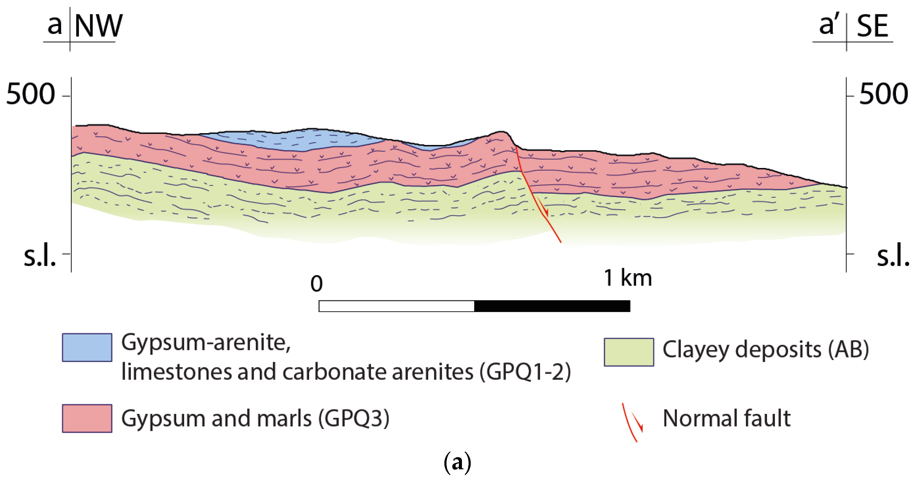
3.1. Geological and Hydrogeological Investigations

To reconstruct the local geology, the stratigraphic logs of 40 geognostic boreholes were considered (Figure 1). In total, 22 out of 40 boreholes were then equipped as piezometers.
The 2D interpretations were uploaded to the three-dimensional geologic modeling software (Move by Petroleum Experts Limited and LeapfrogGeo by Sequent) and the modeling processes allowed the 3D reconstruction of the main geological surface of interest of this work; that is to say, the aquifer bottom. In addition, it was also possible to reconstruct the topographic elevation through official regional cartography and the expected groundwater surface. The latter was obtained by interpolating the location of spring A5 and the hydraulic head measured in observation well D10, thereby estimating the local hydraulic gradient.
Within this study process, the aquifer bottom’s morphology was a nodal issue, considering the need to identify the more probable locations of DNAPL pools. For this reason, once a marked localized depression was clearly identified, a square area of about 50 × 50 m was selected to simulate the DNAPL extraction through pumping, with a grid spacing of 0.1 m.
From November 2021 to May 2022, hydraulic head measurements were carried out monthly using a water level meter. Within the present study, the main aim was to reconstruct the groundwater flow net related to the low-permeability medium outcropping south of the evaporitic aquifer that feeds spring A5 to check possible hydraulic interactions between the two media and then acquire useful information about the origin of the DNAPLs. Therefore, this groundwater flow net was reconstructed using the hydraulic head measured in the only piezometers drilled and screened within the clayey deposits (D12, D13, D13bis, D15, S1, S2, S3, S4, S5, S6, C4, C5, C6, and C7 in Figure 1).
Moreover, taking into account the detection of chlorinated solvents in A5 spring waters during the first observation year, it was decided to continuously measure the hydraulic head fluctuations in piezometer D10 (drilled and screened within the evaporitic aquifer feeding spring A5) during rainfall events, so as to quantify the time lag between precipitation and head rise in a such aquifer. In more detail, he D10 is 36 m deep and was screened between 5 and 35 m below ground. Therefore, in early 2023, a pressure transducer was installed at the bottom of the well in D10, and the hydraulic head was measured on an hourly basis. Contextually, the rainfall was measured in a meteorological station located at the study site hourly.

3.2. Hydrochemical Analyses

Both spring and groundwater samples were collected (at A5 and P10, respectively) from November 2021 to May 2022 on a seasonal basis.
Since a preliminary hydraulic test in D10 suggested low local permeability of the aquifer medium, groundwater sampling was planned to collect samples through a bailer (before purging) and (when possible) through the usual low-flow purging procedure. As a matter of fact, it was possible to collect groundwater samples through the low-flow purging procedure only twice (November 2021 and February 2022). All samples were analyzed in order to acquire information throughout the observation period.
The chemical analyses were carried out by C.A.D.A. s.n.c. (Chimica Applicata Depurazione Acque, società in nome collettivo), a laboratory with ISO 9001:2015, ISO 14001:2015, and ISO 45001:2018 accreditations recognized by the Italian Accreditation Committee (ACCREDIA; accreditation number 0439L).

3.3. Microbiological Analyses: 16S Ribosomal RNA Gene Next-Generation Sequencing (NGS)

The microbiological survey was carried out in November 2021. Water samples (1 L) were filtered through sterile mixed esters of cellulose filters (S-PakTM membrane filters, 47 mm diameter, 0.22 μm pore size; Millipore Corporation, Billerica, MA, USA) within 24 h of collection. The bacterial DNA extraction from the sample filters was performed using the commercial FastDNA SPIN Kit for soil (MP Biomedicals, LLC, Solon, OH, USA) and the FastPrep®Instrument (MP Biomedicals, LLC, Solon, OH, USA). Once the DNA extraction was complete, the quantity and integrity of the DNA were evaluated by electrophoresis in 0.8% agarose gel containing 1 μg/mL of Gel-RedTM (Biotium, Inc., Fremont, CA, USA), in TAE 1X running buffer (40 mM tris base, 20 mM acetic acid, and 1 mM EDTA pH 8), and the amplification reactions were performed by polymerase chain reaction (PCR). The 16S rDNA profiles of the bacterial communities in the samples were obtained using NGS technologies at the Genprobio Srl Laboratory (Parma, Italy). Partial 16S rRNA gene sequences were obtained from the extracted DNA by PCR, using the primer pair of Probio_Uni and/Probio_Rev, which targets the V3 region of the bacterial 16S rRNA gene sequence [38]. The amplifications were carried out using a Verity Thermocycler (Applied Biosystems, Foster City, CA, USA), and the PCR products were purified by magnetic purification using Agencourt AMPure XP DNA purification beads (Beckman Coulter Genomics GmbH, Bernried, Germany) to remove the primer dimers. Amplicon checks were carried out as previously described [47]. The sequencing was performed using an Illumina MiSeq sequencer (Illumina, Hayward, CA, USA) with MiSeq Reagent Kit v3 chemicals. The fastq files were processed using a custom script based on the QIIME software suite [48]. The quality control process retained sequences with lengths between 140 and 400 bp, meaning sequence quality scores >20, whereas sequences with homopolymers >7 bp and mismatched primers were omitted. To calculate downstream diversity measures, operational taxonomic units (OTUs) were defined at 100% sequence homology using DADA2 [49]; OTUs not encompassing at least two sequences of the same sample were removed. All reads were classified to the lowest possible taxonomic rank using QIIME2 [47,50] and a reference dataset from the SILVA database v132 [51].

3.4. Hydrogeological Parameters of the Numerical Model Using CactusHydro

A 3D numerical model was set up using the numerical code CactusHydro, introduced in [CF nature, CF plosone]. CactusHydro resolves the governing partial differential equations that describe the migration of an immiscible phase fluid flow in a porous medium composed of a nonaqueous phase n , water w , and air a and a variably saturated zone. In particular, the spilled DNAPL is considered immiscible, and the effects of the volatilization, biodegradation, or dissolution are not considered. CactusHydro treats the vertical and horizontal movements of the contaminant in the variably saturated zone, which is numerically resolved as a unique zone, together (not separating the vertical movement from the horizontal one, since the flow equation includes both zones). Recent applications of the code can be found in [30,31,35,36,37].
Table 1 and Table 2 show the DNAPL (PCE) phase properties, such as the density, viscosity, porosity, and hydrogeological parameters used in the numerical simulations. In particular, the density of the DNAPL contaminant is ρ n = 1643   kg / m 3 , which is denser than the water, while its viscosity is μ n = 0.844 × 10 3   kg / ms . The simulations were carried out using the PCE as the reference DNAPL because it was the chlorinated organic compound detected at spring A5 with the highest concentration.
Here, we investigate a range of values for the permeability, porosity, and irreducible wetting phase saturation. For the permeability, we choose a range of values for the hydraulic conductivity between K = 10 2 , 10 6   m / s , which corresponds to a minimum value of 1.020 × 10 13   m 2 , and a maximum value of 1.020 × 10 9   m 2 for the permeability in fissured and karstified aquifer media [52]. See Table 1 and Table 2 and the relations between the hydraulic conductivity and permeability and the density and viscosity of water, k = K   μ w ρ w   g .
The porosity range is 0.05 , 0.50 [52]. The irreducible wetting phase saturation range is 0.01 , 0.03 . These are typical values for a residual fracture together with the van Genuchten [53] parameters [54]. See Table 1 and Table 2.
For a three-phase fluid flow, we need two capillary pressures. In our formulation [30,31], we use the air–water phase, p c a w = p a p w , and the capillary pressure for the air–nonaqueous phase p c a n = p a p n . Then, the nonaqueous liquid–water capillary pressure is given by p c n w = p n p w = p c a w p c a n . The relative permeabilities k r w ,   k r n , and k r a and the capillary pressures are a function of the saturations, k r α = k r α S a , S n , S w ,   p c a n = p c a n S a , S n , S w , and p c a w = p c a w S a , S n , S w . The three phases are extended from the two-phase expressions [46] (see [30,31]). For the capillary pressure instead, we use the van Genuchten model [53] (see [30,31]).
The van Genuchten parameter is α = p c ρ w g 1 , where p c is the capillary pressure head. For “sand”, the value is α = 0.145   cm 1 = 14.5   m 1 , and the capillary pressure between the air and water at zero saturation gives p c a w = ρ w g α = 10 3 kg / m 3 9.81   m / s 2 14.5   m 1 = 676.55   Pa .
Using the value of the interfacial tension σ n w = 4.44 × 10 2   N / m and σ a w = 7.199 × 10 2   N / m , we get β n w = σ a w σ n w = 1.62 and p c n w S w = p c a w β n w = 417.62   Pa . Then, the capillary pressure at zero saturation is p c a n = p c a w p c n w = 259.83   Pa .

4. Results

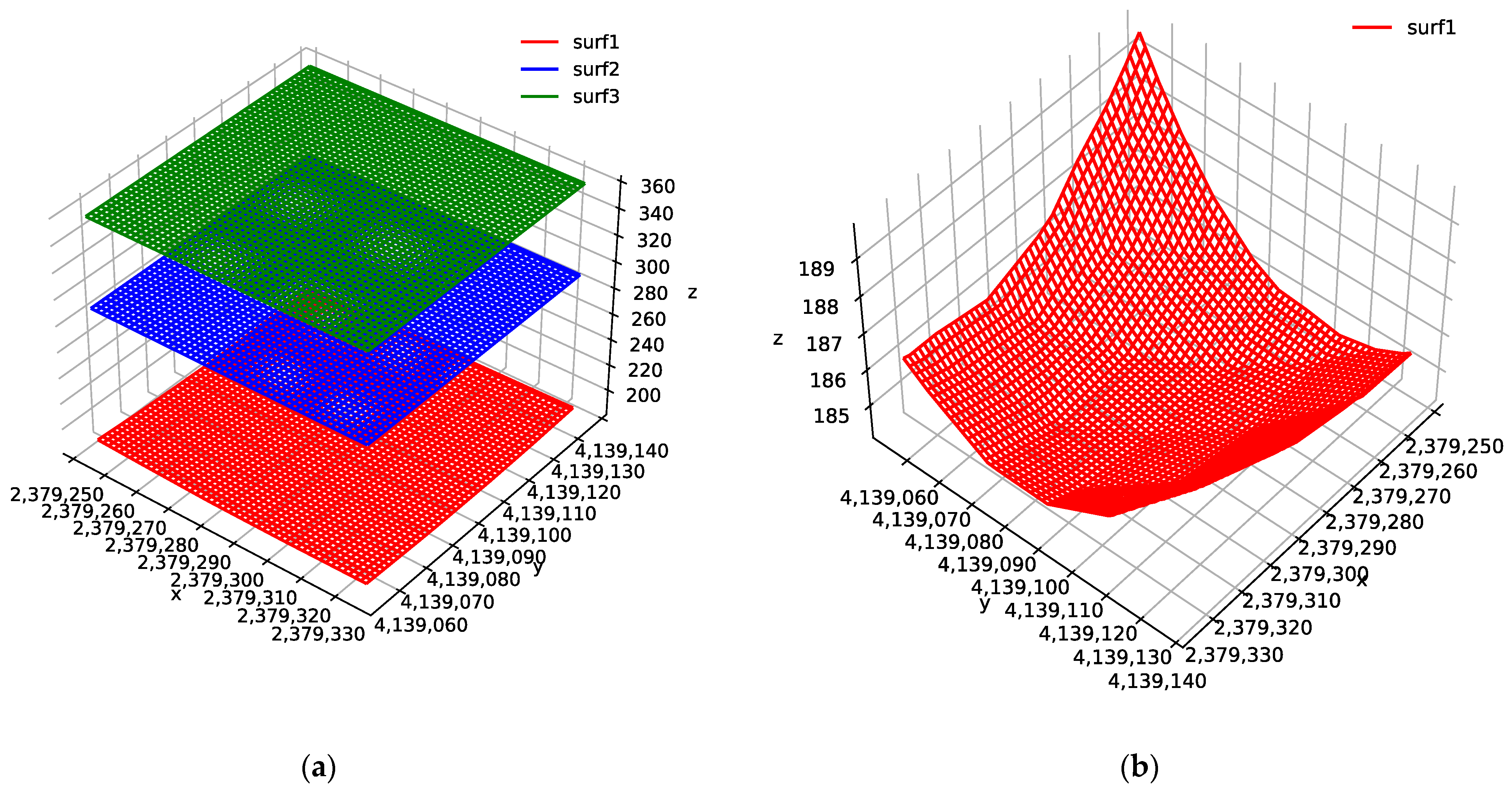
4.1. Morphology of the Bottom Aquitard

Based on the available stratigraphic data and available geologic outcrops, two interpretative profiles extending NW–SE and SW–NE were drawn (Figure 2a,b).
The resulting morphology of the aquifer bottom showed a general SE-ward slope in accordance with the topography trend. In addition to this general arrangement, hectometric elevation changes were recognized in this surface, producing a localized depression toward the hill’s central axis from NW to SE. Inside this central, more depressed area, we recognized a localized further low-relief area, which generated a closed underground basin suitable for a DNAPL pool (Figure 3).

4.2. Hydrogeological Model

As per the low-permeability medium outcropping south of the evaporitic aquifer that feeds spring A5, Figure 4 clearly shows that the local groundwater does not flow toward the evaporites. The SW–NE groundwater divide separates (i) a western subsystem of the clayey medium where the groundwater flows from east to west and then to the south (towards S3) and (ii) an eastern subsystem where the groundwater flows from north-west to the south-east (towards D15). Overall, this groundwater pathway agrees with that reconstructed by Rizzo et al. (2020) [55].
Conversely, within the evaporitic aquifer, the groundwater flows north-west to south-east towards spring A5. This spring is then fed by the effective infiltration within the evaporitic rocks and the surface runoff infiltrating into swallow holes located north of the spring (the red triangle in Figure 4 shows the largest one).

4.3. Hydrochemical Features

Table 3 shows the descriptive statistics results for the physicochemical parameters measured in A5 and D10.
The Langelier–Ludwig diagram indicates that both the spring and groundwater samples belong to the chloride sulfate alkaline earth water type, even if a slight variation can be observed over time (Figure 5). As expected, no significant differences can be observed between the spring and groundwater samples. Moreover, very similar results were obtained for the groundwater samples collected twice in static conditions (through a bailer) and through the usual low-flow purging procedure.
As per the chlorinated organic compounds, slight contamination (tetrachloroethylene [PCE] = 7.9 μg/L; trichloromethane [TCM] = 0.73 μg/L) was detected only in November 2021 at spring A5, close to a heavy precipitation period (cumulative rainfall of 210 mm during the previous 15 days). Conversely, chlorinated organic compounds were never detected in D10 groundwaters during the observation period.

4.4. Microbial Communities

The biomolecular analysis results for the 16S rRNA were deposited in the National Center for Biotechnology Information (NCBI) Sequence Read Archive (SRA) with the project accession number PRJNA967144. Proteobacteria, Firmicutes, and Bacteroidetes represented the three major phyla in the groundwater samples, accounting for, on average, 52%, 22%, and 17% in A5 and 58%, 22%, and 14% in D10, respectively. This abundance was also confirmed at the genus taxonomic level, where genera belonging to these phyla, such as Rhodoferax, Bacteroides, Pseudomonas, and Faecalibacterium, emerged.
Starting from the analysis of the microbial community at the genus level, in both samples, various microbial communities can be observed to which both aerobic and anaerobic or facultative anaerobic bacterial genera belong. Generally, both communities are characterized by mesophilic microorganisms, with some genera characterized by halophilic or halotolerant capacities found in sample D10 or by sulfur-reducing capacities in sample A5. In addition, a large presence of fecal bacteria can also be observed, which appear to be abundant both in the sample of the A5 spring and in the D10 piezometer.
The analysis reveals the presence of bacterial genera that could have metabolic pathways capable of favoring the degradation of chlorinated compounds, such as Rhodoferax and Desulfurivibrio [56,57]. Moreover, from the analysis at the taxonomic species level, the presence of the species Dechloromonas hortensis can be observed, which is associated with the dehalogenation of chlorinated compounds such as PCE [58].

4.5. 3D High-Precision Numerical Simulations Results

The 3D numerical model developed in this study was based on the conceptual model explained in the previous section. It describes the scenario in which a free-product PCE pool lies at the bottom of an aquifer and remains fixed in that position, although there is a hydraulic gradient. It then numerically simulates the pumping extraction through a well using an HRSC conservative flux method and the CactusHydro code introduced in [30,31], with the addition of a module that allows the contaminant’s extraction within a time interval. It is based on the reconstruction through interpolation of the points of two surfaces, the aquifer’s bottom surface (impermeable) and the upper-level surface (ground surface). A third surface located between the previous ones is the groundwater table that separates the unsaturated zone from the saturated aquifer zone. Figure 6a shows these three surfaces, where the green mesh is the ground surface and the blue mesh is the groundwater table surface. The red mesh is the aquifer’s bottom surface, while the larger image of the aquifer’s bottom surface highlights a depression in the aquifer’s base, using the georeferenced coordinates and a grid spacing of 0.1   m .
Initially, we consider a fixed volume for the DNAPL pool (PCE; density ρ n = 1643   kg / m 3 ) positioned in the impermeable aquifer bottom. The contaminant remains located in a single depression in the saturated zone (see Figure 6b). Figure 7 shows the three-dimensional interpolating cubic grid geometry used in this paper. We assume a variably saturated zone to be a parallelepiped measuring 44.0 m long from x = 20.0 , 20.0   m (left-hand side), 40.0 m wide from y = 20.0 , 20.0   m (right-hand side), and 179.0 m deep from z = 181.0 , 360.0   m , for two different times (Figure 7a: t = 0 s; Figure 7b: t = 1 day and 5.0 h). We use a spatial resolution of d x = d y = d z = 1.0   m and a time step size of d t = 0.01   s . We use a three-phase fluid flow (water + DNAPL + air) and the hydrogeological parameters from Table 1. The DNAPL is positioned at x , y , z = 0 , 0 , 185.0   m . The extraction pump is situated at x , y , z = 2 , 0 , 185.0   m . The aquifer medium is composed of a dry zone (and indeed an unsaturated part with S w = 0 ), namely the one depicted in white in Figure 7, and a saturated one, namely the one depicted in blue, separated by a groundwater table surface with a hydraulic gradient of 7.1% towards SE. The green color at the bottom represents the base of the aquifer. The green color on the upper side represents the atmosphere.
The left-hand side of this figure shows the z x plane view (Figure 7a) and the right-hand side shows the z y plane view. The green color on the bottom zone represents the aquifer base. The green line in the upper area represents the atmosphere. The white color is the unsaturated aquifer. The saturated aquifer is colored blue. The scale indicates the values of the saturation contours σ n = S n ϕ , where S n is the saturation of the nonaqueous phase and ϕ is the porosity (whose initial value is given in Table 1).
Figure 7a shows the initial contaminant, which after more than 24 h is completely extracted from the pumping well (Figure 7b).
Since we want to pay attention to the extraction pump, we show a zoomed-in view of Figure 7 of the fate of the DNAPL using the data from Table 1. Figure 8 shows the numerical results of the saturation contours σ n = S n ϕ at different times (Figure 7a: t = 0 s; Figure 7b: t 0.1 h; Figure 7c: t = 0.2 h; Figure 7d: t = 1.1 h.
At t = 0 s (see Figure 8a), there is a cubic volume for the PCE (with the values given in Table 1) and a saturation of S n = 1 . The quantity of the mass at the bottom is equal to 1643   kg / m 3 × 40 × 40 × 179   m 3 × 2.15587709497209 × 10 6 = 1014.5   kg . The extraction pump is situated two meters away in the x-coordinates, so the contaminant starts to move on the right-hand side (see Figure 8b,c) until time t = 1.1 h (panel (d)), where the mass that remains is practically zero. In Figure 8d, the white cube indicates the position of the well and the absence of contaminant.
The pumping rate of the extraction process (contaminant and water) is Q T = 0.000407   m 3 / s = 0.407   L / s . Before starting the pumping process, the value of the saturation multiplied by the porosity is σ n = 2.15587709497209 × 10 6 . After 104611.8 s, the value is σ n = 7.36016960716937 × 10 11 . Its ratio is 3.41 × 10 5 , meaning very few contaminants are left at the bottom of the aquifer.
We also analyzed the numerical case shown in Figure 9, in which the grid geometry is similar to the previous case but the hydrogeological parameters are those from Table 2. We use a spatial resolution of d x = d y = d z = 1.0   m and a time step size of d t = 0.1   s . Since the irreducible wetting saturation is 0.03 (greater than the previous case of 0.01) and the porosity is 0.05 (as the absolute permeability is also four orders of magnitude smaller than in the previous case; compare Table 2 with Table 1), we expect that it will take longer to remove the contaminant.
Figure 10 shows a zoomed-in view of the grid in the region of interest at different times (Figure 10a: t = 0 s.; Figure 10b: t =1.1 h; Figure 10c: t = 2.3 h; Figure 10d: t = 2 days and 8.9 h. Indeed, the pumping rate for the extraction process (contaminant and water) is Q T = 0.000095   m 3 / s = 0.095   L / s . Compared with the previous case, the flow rate in this case is smaller and it takes longer to extract the contaminant. Before pumping, the value of the saturation multiplied by the porosity is σ n = 5.84648044692737 × 10 7 . After 652902.4 s, the value is σ n = 1.30456707252625 × 10 9 . Its ratio is 2.23 × 10 3 , which is still very small but bigger than the previous case.

5. Discussion and Conclusions

A slightly chlorinated organic compound (mainly PCE, subordinately TCM) was detected once at the test site in spring waters during the observation period. Conversely, no pollution was contextually detected in groundwater samples collected in observation well D10 drilled in the feeding aquifer. The episodic detection of PCE and TCM (as a consequence of heavy rainfall), as well as the apparent discrepancy between the spring and groundwater samples in terms of contamination, are congruent with the following scenario: (i) one or more DNAPLs pools lie at the bottom of the investigated aquifer, representing long-term ground and spring water pollution sources; (ii) the plume that originated within the saturated aquifer was not intercepted by the observation well D10; (iii) both the PCE and TCM were detected in spring water but were associated only with huge precipitation; (iv) the magnitude of the pressure head increase at the aquifer bottom consequent to an unusual recharge event (210 mm in 15 days) was able to cause the significantly increased mobilization and flow of deep (contaminated) groundwater towards the spring; (v) as a result, an unusually high volume of deep (contaminated) groundwater temporarily flowed out at spring A5, high enough to be detected.
The effectiveness of this interpretation was further supported by analyzing the hydraulic head rise on an hourly basis in D10 in early 2023. As shown in Figure 11, (i) the 23.8 mm of rainfall in 12 h between 9 February 2023 and 10 February 2023 caused a fast (about 7 h of time lag) rise (about 0.4 m) in the groundwater head, while (ii) the 28.4 mm of rainfall in 3 h on 3 March 2023 caused a rapid (about 8 h of time lag) rise (about 0.5 m) in the hydraulic head. Based on these data and supposing a linear relationship between the data, the 210 mm precipitation event that preceded the only PCE and TCM detection instance in spring waters during the observation period should have caused an unusual and huge head rise in the order of several meters at D10.
Considering the conceptual model described before, three-dimensional numerical modeling was successfully implemented to predict the efficacy of free-product PCE extraction through a pumping well in the test aquifer. We followed the numerical results based on the saturation contours of the three-phase immiscible fluid flow formed by water, DNAPL, and air in dry soil at different times, using the CactusHydro [30,31] conservative HRSC method, which precisely follows the advective part of the fluid flow and resolves the hyperbolic part of the nonlinear governing coupled equations of a three-phase immiscible fluid flow.
Taking into consideration the morphology of the bottom aquiclude (purposely reconstructed through a detailed geological characterization of the test site) and the existence of a unique depression where the DNAPL pool could be located, the numerical model was not used to simulate the DNAPL’s migration to the subsurface once released in the environment. Instead, we simulated the effects of the pumping well screened at the bottom of the pool to recover the contaminant. The results indicated that CactusHydro can precisely follow the contaminant’s fate and its recovery using a pumping well. Moreover, the simulation model showed that the free-product pumping recovered almost the whole DNAPL pool, even though a slight difference in the recovery percentages can be expected depending on the hydraulic features of the aquifer medium.
Taking into consideration the results of the numerical simulation, the pumping solution could avoid a significant volume of free product acting as a long-term pollution source. At the same time, the existence of an autochthonous microbial community able to degrade chlorinated solvents will promote natural attenuation processes within the groundwater matrix.
The limitations of the numerical model are that at this stage (i) we consider these fluids (groundwater and PCE) immiscible, and the process of volatilization or dissolution was not considered, while (ii) the hydraulic parameters of the aquifer medium (permeability, porosity, irreducible water saturation) did not refer to the specific test site but were taken from the scientific literature. However, both limitations are acceptable at the planning stage of this type of research on heterogeneous aquifer media because they are normally finalized to optimize the interdisciplinary approach in order to respond to some basic questions: (i) Do we expect that hydraulic heterogeneities to significantly influence the free-product DNAPL extraction? (ii) If so, that is the expected range of free-product DNAPL recovery rates as a function of the expected aquifer heterogeneity? (iii) Is it necessary to design and apply bioremediation techniques associated with free-product extraction or can the natural attenuation provided by the autochthonous microbial community be considered enough to efficaciously remove the pollution source? Additionally, the field site is contaminated with both PCE and TCM and the numerical model used here does not differentiate between single-component and multicomponent DNAPLs. We plane to include more than one nonaqueous phase liquid in the future.
As per the last issue, coupling the numerical simulations of the study site to the bacterial community characterization, we were effectively able to predict that (i) the PCE recovery through a pumping well will be almost completed and (ii) the application of other remediation techniques (such as bioremediation) is not necessary to remove the pollution source because (iii) a natural attenuation process is provided by the autochthonous bacterial community, which is characterized by genera (such as Dechloromonas, Rhodoferax, and Desulfurivibrio) that could have metabolic pathways capable of favoring the degradation of chlorinated compounds.
In a wider context, this study demonstrates that a coupled experimental modeling approach, based on results obtained from an interdisciplinary perspective, is an effective way to synergically plan and design both short- (pumping well) and medium-term (e.g., natural attenuation) solutions to remove DNAPL pools from aquifer systems efficaciously.

Author Contributions

Conceptualization, A.F., E.R. and F.C.; methodology, A.F., F.L.M., P.R., M.G.M., R.P., E.R. and F.C.; software, F.L.M., M.G.M. and R.P.; validation, A.F., E.R. and F.C.; formal analysis, A.F., F.L.M., P.R., M.G.M., R.P., E.R. and F.C.; investigation, F.L, P.R. and M.G.M..; resources, F.L.M., P.R., M.G.M. and R.P.; data curation, F.L.M., P.R., M.G.M. and R.P.; writing—original draft preparation, A.F., F.L.M., P.R., M.G.M., R.P., E.R. and F.C.; writing—review and editing, A.F., F.L.M., E.R. and F.C.; visualization, A.F., F.L.M., M.G.M. and R.P.; supervision, E.R. and F.C.; project administration, E.R. and F.C.; funding acquisition, E.R. and F.C. All authors have read and agreed to the published version of the manuscript.

Funding

This research was funded by Catanzaro Costruzioni S.r.l. (Heads of Funds: E. Rotigliano, F. Celico).

Data Availability Statement

The data are contained within the article.

Acknowledgments

We warmly acknowledge Fabio Catanzaro, Salvatore Accardo, and Rosario Varsalona for their useful discussions. This work used high-performance-computing resources at the University of Parma (https://www.hpc.unipr.it) accessed on 1 January 2023. This work benefited from the equipment and framework of the COMP-R Initiative, funded by the ‘Departments of Excellence’ program of the Italian Ministry for Education, University, and Research (MIUR, 2023–2027). A.F. and F.C. acknowledge the financial support from the PNRR MUR project ECS_00000033_ECOSISTER. We also thank the two anonymous reviewers for their valuable comments and questions.

Conflicts of Interest

The authors declare no conflict of interest.

References

  1. Mercer, J.W.; Cohen, R.M. A review of immiscible fluids in the subsurface: Properties, models, characterization and remediation. J. Contam. Hydrol. 1990, 6, 107–163. [Google Scholar] [CrossRef]
  2. Henschler, D. Toxicity of chlorinated organic compounds: Effects of the introduction of chlorine in organic molecules. Angew. Chem. 1994, 33, 1920–1935. [Google Scholar] [CrossRef]
  3. Volpe, A.; Del Moro, G.; Rossetti, S.; Tandoi, V.; Lopez, A. Remediation of PCE-contaminated groundwater from an industrial site in southern Italy: A laboratory-scale study. Process Biochem. 2007, 42, 1498–1505. [Google Scholar] [CrossRef]
  4. Lyman, W.; Reehl, W.; Rosenblatt, D. Handbook of Chemical Properties Estimation Methods-Environmental Behavior of Organic Compound; McGraw-Hill: New York, NY, USA, 1982. [Google Scholar]
  5. Mackay, D.; Roberts, P.; Cherry, J. Transport of organic contaminants in groundwater. Environ. Sci. Technol. 1985, 19, 384–392. [Google Scholar] [CrossRef] [PubMed]
  6. Parker, J.C.; Lenhard, R.J.; Kuppusamy, T. A parametric model for constitutive properties governing multi-phase flow in porous media. Water Resour Res. 1987, 23, 618–624. [Google Scholar] [CrossRef]
  7. Kueper, B.; Frind, E. An overview of immiscible fingering in porous media. J. Contam. Hydrol. 1988, 2, 95–110. [Google Scholar] [CrossRef]
  8. Kueper, B.; Abbott, W.; Farquhar, G. Experimental observations of multiphase flow in heterogeneous porous media. J. Contam. Hydrol. 1989, 5, 83–95. [Google Scholar] [CrossRef]
  9. Kueper, B.; Frind, E.O. Two-phase flow in heterogeneous porous media: 2. Model application. Water Resour. Res. 1991, 27, 1059–1070. [Google Scholar] [CrossRef]
  10. Parker, J. Multiphase flow and transport in porous media. Rev. Geophys. 1989, 27, 311–328. [Google Scholar] [CrossRef]
  11. Hirata, T.; Muraoka, K. Vertical migration of chlorinated organic compounds in porous media. Water Res. 1988, 22, 481–484. [Google Scholar] [CrossRef]
  12. Ahmadi, H.; Kilanehei, F.; Nazari-Sharabian, M. Impact of Pumping Rate on Contaminant Transport in Groundwater—A Numerical Study. Hydrology 2021, 8, 103. [Google Scholar] [CrossRef]
  13. McLaren, R.G.; Sudicky, E.A.; Park, Y.-J.; Illman, W.A. Numerical simulation of DNAPL emissions and remediation in a fractured dolomitic aquifer. J. Contam. Hydrol. 2012, 136, 56–71. [Google Scholar] [CrossRef] [PubMed]
  14. Guadaño, J.; Gómez, J.; Fernández, J.; Lorenzo, D.; Domínguez, C.M.; Cotillas, S.; García-Cervilla, R.; Santos, A. Remediation of the Alluvial Aquifer of the Sardas Landfill (Sabiñánigo, Huesca) by Surfactant Application. Sustainability 2022, 14, 16576. [Google Scholar] [CrossRef]
  15. Zhou, J.; Song, B.; Yu, L.; Xie, W.; Lu, X.; Jiang, D.; Kong, L.; Deng, S.; Song, M. Numerical Research on Migration Law of Typical Chlorinated Organic Matter in Shallow Groundwater of Yangtze Delta Region. Water 2023, 15, 1381. [Google Scholar] [CrossRef]
  16. Zheng, C.; Wang, P.P. MT3DMS: A Modular Three-Dimensional Multispe-cies Transport Model for Simulation of Advection, Dispersion, and Chemical Reactions of Contaminants in Groundwater Systems. In Documentation and User’s Guide; No. SERDP-99-1; U.S. Army Engineer Research and Development Center: Vicksburg, MS, USA, 1999. [Google Scholar]
  17. Anderson, M.R.; Johnson, R.L.; Pankow, J.K. Dissolution of Dense Chlorinated Solvents into Groundwater. 3. Modeling Contaminant Plumes from Fingers and Pools of Solvent. Environ. Sci. Technol. 1992, 26, 901–908. [Google Scholar] [CrossRef]
  18. Johnson, R.L.; Pankov, J.F. Dissolution of Dense Chlorinated Solvents into Groundwater. 2. Source Functions for Pools of Solvent. Environ. Sci. Technol. 1992, 26, 896–901. [Google Scholar] [CrossRef]
  19. Roy, J.W.; Smith, J.E.; Gillham, R.W. Laboratory evidence of natural remobilization of multicomponent DNAPL pools due to dissolution. J. Contam. Hydrol. 2004, 74, 145–161. [Google Scholar] [CrossRef]
  20. Seagren, E.A.; Rittmann, B.E.; Valocchi, A.J. An experimental investigation of NAPL pool dissolution enhancement by flushing. J. Contam. Hydrol. 1999, 37, 111. [Google Scholar] [CrossRef]
  21. Chrysikopoulos, C.V.; Voudrias, E.A.; Fyrillas, M.M. Modeling of contaminant transport resulting from dissolution of nonaqueous phase liquid pools in saturated porous media. Transp. Porous Med. 1994, 16, 125–145. [Google Scholar] [CrossRef]
  22. Chrysikopoulos, C.V. Three-dimensional analytical models of contaminant transport from nonaqueous phase liquid pool dissolution in saturated subsurface formation. Water Resour. Res. 1995, 31, 1137–1145. [Google Scholar] [CrossRef]
  23. Kenneth, Y.L.; Chrysikopoulos, C.V. Dissolution of a multicomponent of DNAPL pool in an experimental aquifer. J. Hazard. Mater. 2006, B128, 218–226. [Google Scholar]
  24. Soga, K.; Page, J.W.E.; Illangasekare, T.H. A review of NAPL source zone remediation efficiency and the mass flux approach. J. Hazard. Mater. 2014, 110, 13–27. [Google Scholar] [CrossRef] [PubMed]
  25. Essaid, H.; Bekins, B.A.; Cozzarelli, I.M. Organic contaminant transport and fate in the subsurface: Evolution of knowledge and understanding. Water Resour. Res. 2015, 51, 4861–4902. [Google Scholar] [CrossRef]
  26. Praseeja, A.V.; Sajikumar, N. A review on the study of immiscible fluid flow in unsaturated porous media: Modeling and remediation. J. Porous Media 2019, 22, 889–922. [Google Scholar] [CrossRef]
  27. Ahmed, M.; Saleem, M.R.; Zia, S.; Qamar, S. Central Upwind Scheme for a Compressible Two-Phase Flow Model. PLoS ONE 2015, 10, e0126273. [Google Scholar] [CrossRef] [PubMed]
  28. Pandare, A.K.; Waltz, J.; Bakosi, J. A reconstructed discontinuous Galerkin method for multi-material hydrodynamics with sharp interfaces. Int. J. Numer. Methods Fluids 2020, 92, 874–889. [Google Scholar] [CrossRef]
  29. Kuchařík, M.; Liska, R.; Steinberg, S.; Wendroff, B. Optimally-stable second-order accurate difference schemes for non-linear conservation laws in 3D. Appl. Numer. Math. 2006, 56, 589–607. [Google Scholar] [CrossRef]
  30. Feo, A.; Celico, F. High-resolution shock-capturing numerical simulations of three-phase immiscible fluids from the unsaturated to the saturated zone. Sci. Rep. 2021, 11, 5212. [Google Scholar] [CrossRef]
  31. Feo, A.; Celico, F. Investigating the migration of immiscible contaminant fluid flow in homogeneous and heterogeneous aquifers with high-precision numerical simulations. PLoS ONE 2022, 17, e0266486. [Google Scholar] [CrossRef]
  32. Kurganov, A.; Tadmor, E. New high-resolution central scheme for non-linear conservation laws and convection-diffusion equations. J. Comput. Phys. 2000, 160, 241–282. [Google Scholar] [CrossRef]
  33. Lax, P.; Wendroff, B. Systems of conservation laws. Commun. Pure Appl. Math. 1960, 3, 217–237. [Google Scholar] [CrossRef]
  34. Hou, T.Y.; LeFloch, P.G. Why nonconservative schemes converge to wrong solutions: Error analysis. Math. Comp. 1994, 62, 497–530. [Google Scholar] [CrossRef]
  35. Feo, A.; Celico, F.; Zanini, A. Migration of DNAPL in Saturated Porous Media: Validation of High-Resolution Shock-Capturing Numerical Simulations through a Sandbox Experiment. Water 2023, 15, 1471. [Google Scholar] [CrossRef]
  36. Feo, A.; Pinardi, R.; Scanferla, E.; Celico, F. How to Minimize the Environmental Contamination Caused by Hydrocarbon Releases by Onshore Pipelines: The Key Role of a Three-Dimensional Three-Phase Fluid Flow Numerical Model. Water 2023, 15, 1900. [Google Scholar] [CrossRef]
  37. Feo, A.; Pinardi, R.; Artoni, A.; Celico, F. Three-Dimensional High-Precision Numerical Simulations of Free-Product DNAPL Extraction in Potential Emergency Scenarios: A Test Study in a PCE-Contaminated Alluvial Aquifer (Parma, Northern Italy). Sustainability 2023, 15, 9166. [Google Scholar] [CrossRef]
  38. Pinardi, R.; Feo, A.; Ruffini, A.; Celico, F. Purpose-Designed Hydrogeological Maps for Wide Interconnected Surface–Groundwater Systems: The Test Example of Parma Alluvial Aquifer and Taro River Basin (Northern Italy). Hydrology 2023, 10, 127. [Google Scholar] [CrossRef]
  39. Allen, G.; Goodale, T.; Lanfermann, G.; Radke, T.; Rideout, D.; Thornburg, J. Cactus Users’ Guide. 2011. Available online: http://www.cactuscode.org/documentation/UsersGuide.pdf (accessed on 1 January 2023).
  40. Cactus Developers. Cactus Computational Toolkit. Available online: http://www.cactuscode.org (accessed on 1 January 2023).
  41. Goodale, T.; Allen, G.; Lanfermann, G.; Massó, J.; Radke, T.; Seidel, E.; Shalf, J. The Cactus Framework and Toolkit: Design and Applications. In Vector and Parallel Processing—VECPAR’2002, Proceedings of the 5th International Converence, Porto, Portugal, 26–28 June 2002; Lecture Notes in Computer Science; Springer: Berlin, Germany, 2003; Available online: http://edoc.mpg.de/3341 (accessed on 1 January 2023).
  42. Schnetter, E.; Hawley, S.H.; Hawke, I. Evolutions in 3D numerical relativity using fixed mesh refinement. Class. Quantum Gravity 2004, 21, 1465–1488. [Google Scholar] [CrossRef]
  43. Schnetter, E.; Diener, P.; Dorband, E.N.; Tiglio, M. A multi-block infrastructure for three-dimensional time-dependent numerical relativity. Class. Quantum Gravity 2006, 23, S553. [Google Scholar] [CrossRef]
  44. Gugliotta, C.; Gasparo Morticelli, M.; Avellone, G.; Agate, M.; Barchi, M.R.; Albanese, C.; Valenti, V.; Catalano, R. Middle Miocene—Early Pliocene wedge-top basins of North-Western Sicily (Italy). Constraints for the tectonic evolution of a “non-conventional” thrust belt, affected by transpression. J. Geol. Soc. Lond. 2014, 171, 211–226. [Google Scholar] [CrossRef]
  45. Catalano, R.; Valenti, V.; Albanese, C.; Accaino, F.; Sulli, A.; Tinivella, U.; Gasparo Morticelli, M.; Zanolla, C.; Giustiniani, M. Sicily’s fold/thrust belt and slab rollback: The SI. RI.PRO. seismic crustal transect. J. Geol. Soc. Lond. 2013, 170, 451–464. [Google Scholar]
  46. Cappadonia, C.; Coratza, P.; Agnesi, V.; Soldati, M. Malta and Sicily joined by geoheritage enhancement and geotourism within the framework of land management and development. Swiss. J. Geosci. 2018, 8, 253. [Google Scholar] [CrossRef]
  47. Milani, C.; Hevia, A.; Foroni, E.; Duranti, S.; Turroni, F.; Lugli, G.A.; Sanchez, B.; Martín, R.; Gueimonde, M.; van Sinderen, D.; et al. Assessing the Fecal Microbiota: An Optimized Ion Torrent 16S rRNA Gene-Based Analysis Protocol. PLoS ONE 2013, 8, e68739. [Google Scholar] [CrossRef]
  48. Caporaso, J.G.; Kuczynski, J.; Stombaugh, J.; Bittinger, K.; Bushman, F.D.; Costello, E.K.; Fierer, N.; Gonzalez Peña, A.; Goodrich, J.K.; Gordon, J.I.; et al. QIIME allows analysis of high-throughput community sequencing data. Nat. Methods 2010, 7, 335–336. [Google Scholar] [CrossRef]
  49. Callahan, B.J.; McMurdie, P.J.; Rosen, M.J.; Han, A.W.; Johnson, A.J.; Holmes, S.P. DADA2: High-resolution sample inference from Illumina amplicon data. Nat. Methods 2016, 13, 581–583. [Google Scholar] [CrossRef]
  50. Bokulich, N.A.; Kaehler, B.D.; Rideout, J.R.; Dillon, M.; Bolyen, E.; Knight, R.; Huttley, G.A.; Caporaso, G.J. Optimizing taxonomic classification of marker-gene amplicon sequences with QIIME 2′s q2-feature-classifier plugin. Microbiome 2018, 6, 90. [Google Scholar] [CrossRef]
  51. Quast, C.; Pruesse, E.; Yilmaz, P.; Gerken, J.; Schweer, T.; Yarza, P.; Peplies, J.; Glöckner, F.O. The SILVA ribosomal RNA gene database project: Improved data processing and web-based tools. Nucleic Acids Res. 2012, 41, 590–596. [Google Scholar] [CrossRef] [PubMed]
  52. Freeze, R.A.; Cherry, J.A. Groundwater Book; Prentice-Hall Inc.: Englewood Cliffs, NJ, USA, 1979. [Google Scholar]
  53. Van Genuchten, M.T. A closed form equation for predicting the hydraulic conductivity of unsaturated soils. Soil Sci. Soc. Am. J. 1980, 44, 892–898. [Google Scholar] [CrossRef]
  54. Yu-Shu, W. Multiphase Fluid Flow in Porous and Fractured Reservoirs; Elsevier: Oxford, UK, 2015; p. 243. [Google Scholar]
  55. Rizzo, P.; Cappadonia, C.; Rotigliano, E.; Iacumin, P.; Sanangelantoni, A.M.; Zerbini, G.; Celico, F. Hydrogeological behaviour and geochemical features of waters in evaporite-bearing low-permeability successions: A case study in Southern Italy. Appl. Sci. 2020, 10, 8177. [Google Scholar] [CrossRef]
  56. Zaa, C.L.Y.; McLean, J.E.; Dupont, R.R.; Norton, J.M.; Sorensen, D.L. Dechlorinating and iron reducing bacteria distribution in a TCE-contaminated aquifer. Groundw. Monit. Remediat. 2010, 30, 46–57. [Google Scholar] [CrossRef]
  57. Della-Negra, O.; Chaussonnerie, S.; Fonknechten, N.; Barbance, A.; Muselet, D.; Martin, D.E.; Fouteau, S.; Fischer, C.; Saaidi, P.-L.; Le Paslier, D. Transformation of the recalcitrant pesticide chlordecone by Desulfovibrio sp. 86 with a switch from ring-opening dechlorination to reductive sulfidation activity. Sci. Rep. 2020, 10, 13545. [Google Scholar] [CrossRef]
  58. Wolterink, A.; Kim, S.; Muusse, M.; Kim, I.S.; Roholl, P.J.; van Ginkel, C.G.; Stams, A.J.M.; Kengen, S.W. Dechloromonas hortensis sp. nov. and strain ASK-1, two novel (per) chlorate-reducing bacteria, and taxonomic description of strain GR-1. Int. J. Syst. Evol. Microbiol. 2005, 55, 2063–2068. [Google Scholar] [CrossRef] [PubMed]
Figure 1. Geological map.
Hydrology 10 00143 g001
Figure 2. (a) Geological section oriented NW–SE (see location in Figure 1) (b). Geological section oriented SW–NE (see location in Figure 1).
Hydrology 10 00143 g002aHydrology 10 00143 g002b
Figure 3. Morphology of the evaporitic aquifer bottom (green dots: bottom of the evaporitic aquifer; red polygon: localized depression in the bottom of the aquifer, utilized for the numerical model; Y-axis green line: NS axis with coordinates in the reference system Rome_1940_Gauss_Boaga; X-axis red line: EW axis with coordinates in the reference system Rome_1940_Gauss_Boaga; Z-axis blue line: elevations in m asl). The view is from the SE, as indicated by the reference globe above the scale. Vertical exaggeration = 3×. Images generated by LeapfrogGeo version 2021.1.3.
Hydrology 10 00143 g003
Figure 4. Hydrogeological sketch.
Hydrology 10 00143 g004
Figure 5. Lamgelier–Ludwig diagram.
Hydrology 10 00143 g005
Figure 6. The three surfaces with georeferenced coordinates: (a) the three surfaces, i.e., the aquifer’s bottom surface (surf2-red), the upper-level topographic surface (surf1-green), and the groundwater table surface (surf3-blue); (b) a larger image of the aquifer’s bottom surface that highlights a depression in the impermeable base with the contaminant’s location.
Hydrology 10 00143 g006
Figure 7. The three-dimensional interpolated grid geometry used in the numerical simulation of a three-phase fluid flow (water + DNAPL + air) and the hydrogeological parameters of Table 1, with a spatial grid resolution of 1.0   m and grid dimensions of 40   × 40   × 179   m , for two different times: (a) t = 0 s; (b) t = 1 day and 5.0 h. The immiscible contaminant is situated at the bottom of the interpolating cubic grid (see the z x and z y plane views). The green color in the bottom zone represents the aquifer base. The green line in the upper area represents the atmosphere. The white color is the unsaturated zone. The blue color is the saturated aquifer.
Hydrology 10 00143 g007
Figure 8. Three-dimensional numerical results of the saturation contours σ n = S n ϕ of the DNAPL using the hydrogeological parameters from Table 1 at different times: (a) t = 0 s; (b) t 0.1 h; (c) t = 0.2 h; (d) t = 1.1 h. The red and blue arrows denote the flow direction of σ n and σ w , respectively.
Hydrology 10 00143 g008
Figure 9. The three-dimensional interpolated grid geometry used in the numerical simulation of a three-phase fluid flow (water + DNAPL + air) and the hydrogeological parameters from Table 2, with a spatial grid resolution of 1.0   m and a grid dimension of 40   × 40   × 179   m for two different times: (a) t = 0 s; (b) t = 7 days and 13.1 h. The immiscible contaminant is situated at the bottom of the interpolating cubic grid (see the z x and z y plane views). The green color in the bottom zone represents the aquifer base. The green line in the upper area represents the atmosphere. The white color is the unsaturated zone. The blue color the saturated aquifer.
Hydrology 10 00143 g009
Figure 10. Three-dimensional numerical results for the saturation contours σ n = S n ϕ of the DNAPL using the hydrogeological parameters from Table 2 at different times: (a) t = 0 s; (b) t = 1.1 h; (c) t = 2.3 h; (d) t = 2 days and 8.9 h.
Hydrology 10 00143 g010
Figure 11. Hydraulic head in D10 (blue line) vs. rainfall (black bars) on an hourly basis (dates are given in year-month-day-hour).
Hydrology 10 00143 g011
Table 1. Definitions of the parameters used in the numerical simulations of DNAPL (PCE) migration and the values of three parameters (maximum absolute permeability, maximum porosity, and minimal irreducible water phase saturation).
ParameterSymbolValue
Absolute permeability (max) k max 1.020 × 10 9   m 2
Rock compressibility c R 4.35 × 10 7 Pa 1
Porosity (max) ϕ 0 , m a x 0.50
Water viscosity μ w 10 3   kg / ms
Water density ρ w 10 3 kg / m 3
DNAPL viscosity μ n 0.844 × 10 3   kg / ms
DNAPL density ρ n 1643   kg / m 3
Air viscosity μ a 1.8 × 10 5 kg / ms
Air density ρ a 1.225   kg / m 3
Van Genuchten n , m 2.57 , 1 1 2.57
Irreducible wetting phase saturation (min) S w i r , m i n 0.010
Surface tension of air–water σ a w 7.199 × 10 2   N / m
Interfacial tension nonaqueous water σ n w 4.44 × 10 2   N / m
Capillary pressure of air–water at zero saturation p c a w 0 676.55   Pa
Capillary pressure of air–nonaqueous phase at zero saturation p c a n 0 259.83   Pa
Table 2. Definitions of the parameters used in the numerical simulations of DNAPL (PCE) migration and the values of three parameters (minimal absolute permeability, minimal porosity, and maximum irreducible water phase saturation).
ParameterSymbolValue
Absolute permeability (min) k m i n 1.020 × 10 13   m 2
Rock compressibility c R 4.35 × 10 7   Pa 1
Porosity (min) ϕ 0 , m i n 0.05
Water viscosity μ w 10 3   kg / ms
Water density ρ w 10 3 kg / m 3
DNAPL viscosity μ n 0.844 × 10 3   kg / ms
DNAPL density ρ n 1643   kg / m 3
Air viscosity μ a 1.8 × 10 5   kg / ms
Air density ρ a 1.225   kg / m 3
Van Genuchten n , m 2.57 , 1 1 2.57
Irreducible wetting phase saturation (max) S w i r , m a x 0.030
Surface tension of air–water σ a w 7.199 × 10 2   N / m
Interfacial tension nonaqueous water σ n w 4.44 × 10 2   N / m
Capillary pressure of air–water at zero saturation p c a w 0 676.55   Pa
Capillary pressure of air–nonaqueous phase at zero saturation p c a n 0 259.83   Pa
Table 3. Physicochemical parameters of spring (A5) and groundwaters (D10) (Min is the minimum value; Max is the maximum value; D.ST. is the standard deviation; 25Q is the 1st quartile; 75Q is the 3rd quartile; 10P is the 10th percentile; 90P is the 90th percentile; C.V. is the coefficient of variation).
AverageMedianMinMaxD.ST.25Q75Q10P90PC.V
A5T20.1620.816.5023.22.0719.221.2017.3021.68971.67
pH6.977.246.187.480.496.447.326.377.361426.26
Eh312.6718946.901572479.08100239.1055.22522.2465.26
Ec3.502.3640.709.9372.821.634.031.426.36124.06
D10T19.8820.116.1022.81.7519.820.5018.4220.961133.66
pH7.267.066.688.340.546.997.326.877.971334.70
Eh254.28130.951.00522.5188.34109.1427.6070.28451.22135.01
Ec3.373.501.825.3081.042.683.732.364.26322.92
Disclaimer/Publisher’s Note: The statements, opinions and data contained in all publications are solely those of the individual author(s) and contributor(s) and not of MDPI and/or the editor(s). MDPI and/or the editor(s) disclaim responsibility for any injury to people or property resulting from any ideas, methods, instructions or products referred to in the content.

