
Impacts of Max-Stable Process Areal Exceedance Calculations to Study Area Sampling Density, Surface Network Precipitation Gage Extent and Density, and Model Fitting Method

Abstract
:1. Introduction
2. Materials and Methods
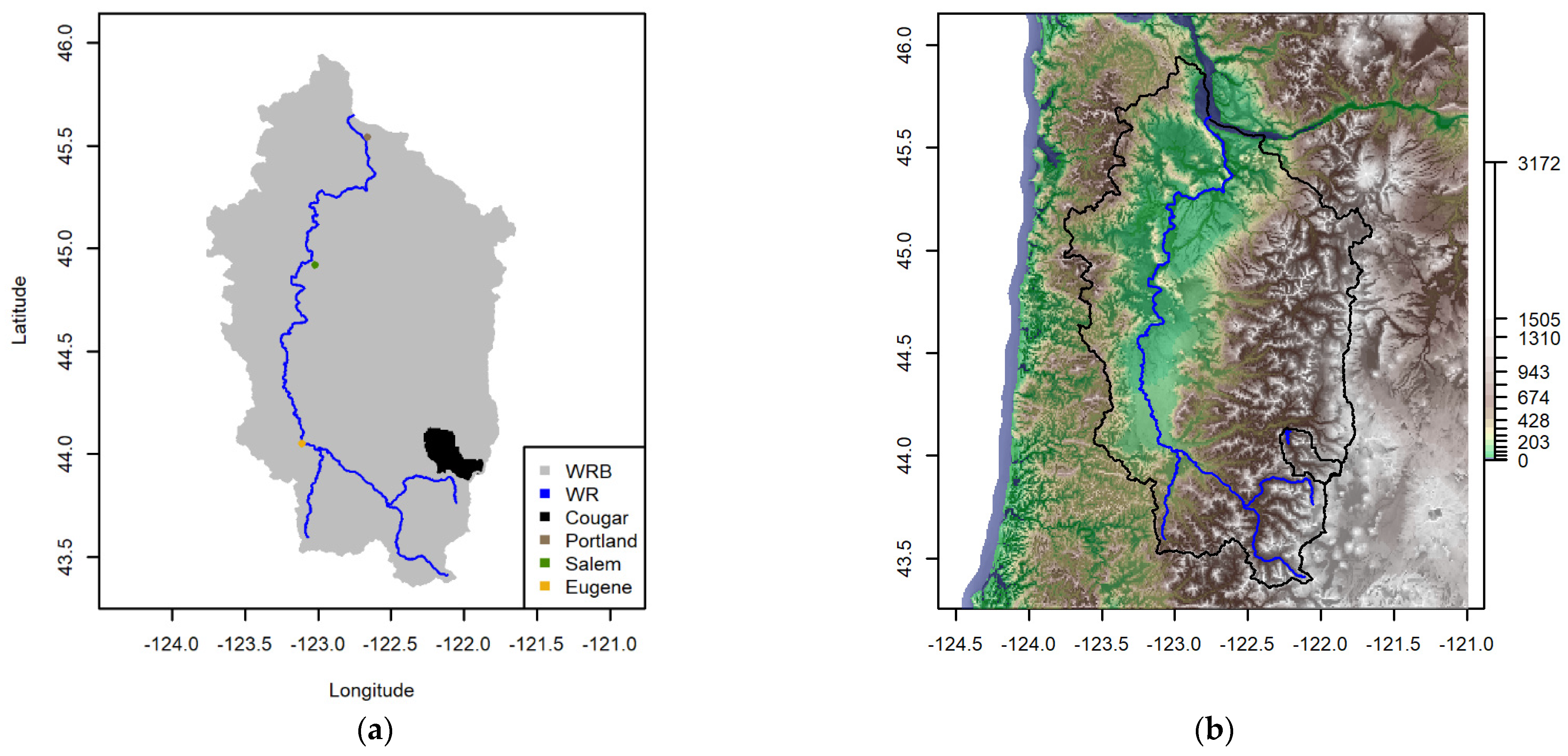
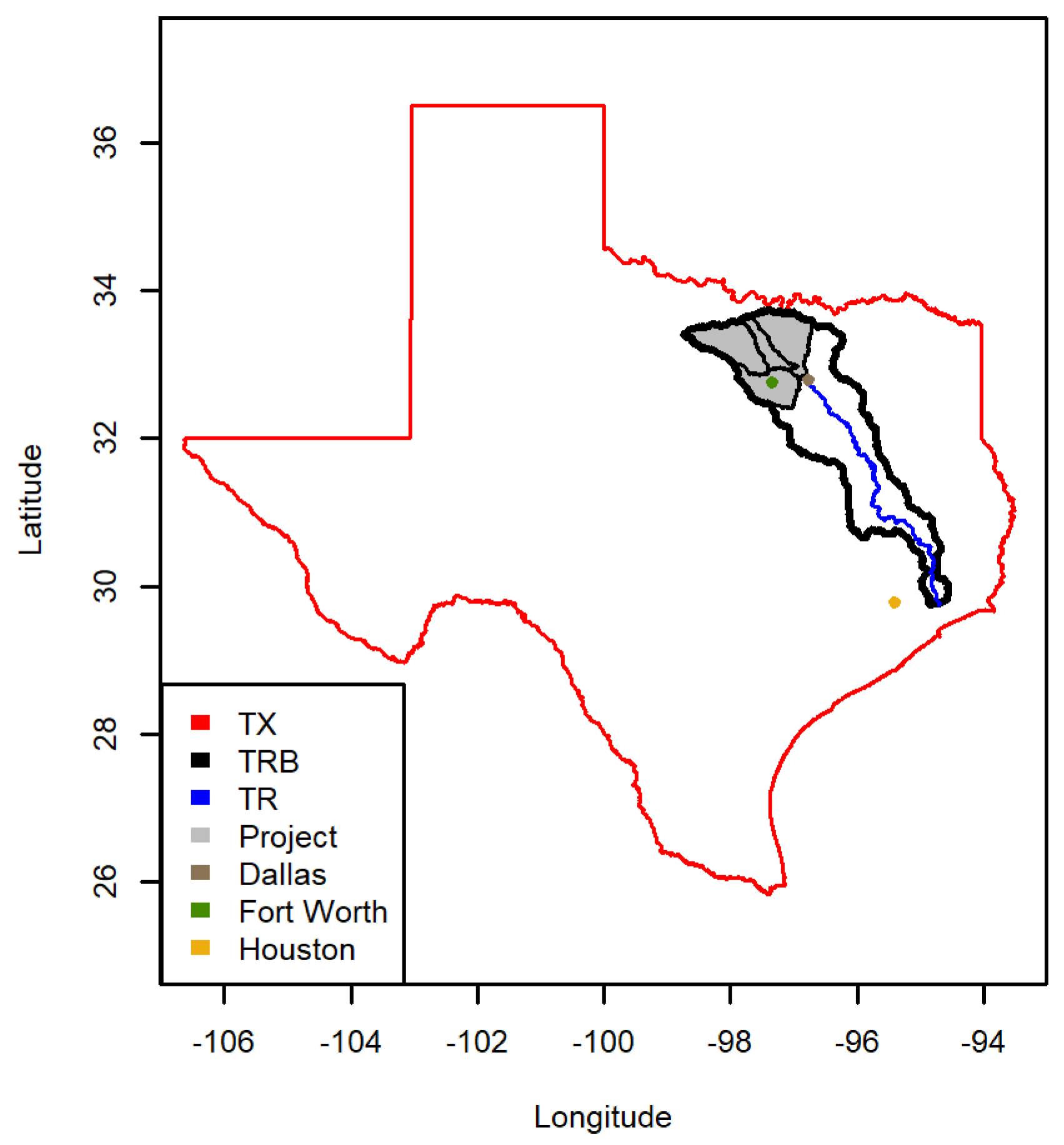
2.1. Study Areas
2.2. Block Maxima Precipitation Datasets
2.3. Gridded Covariate Data
2.4. Methods
2.4.1. Impact of MSP Areal Exceedance Calculations to Study Area Sampling Density
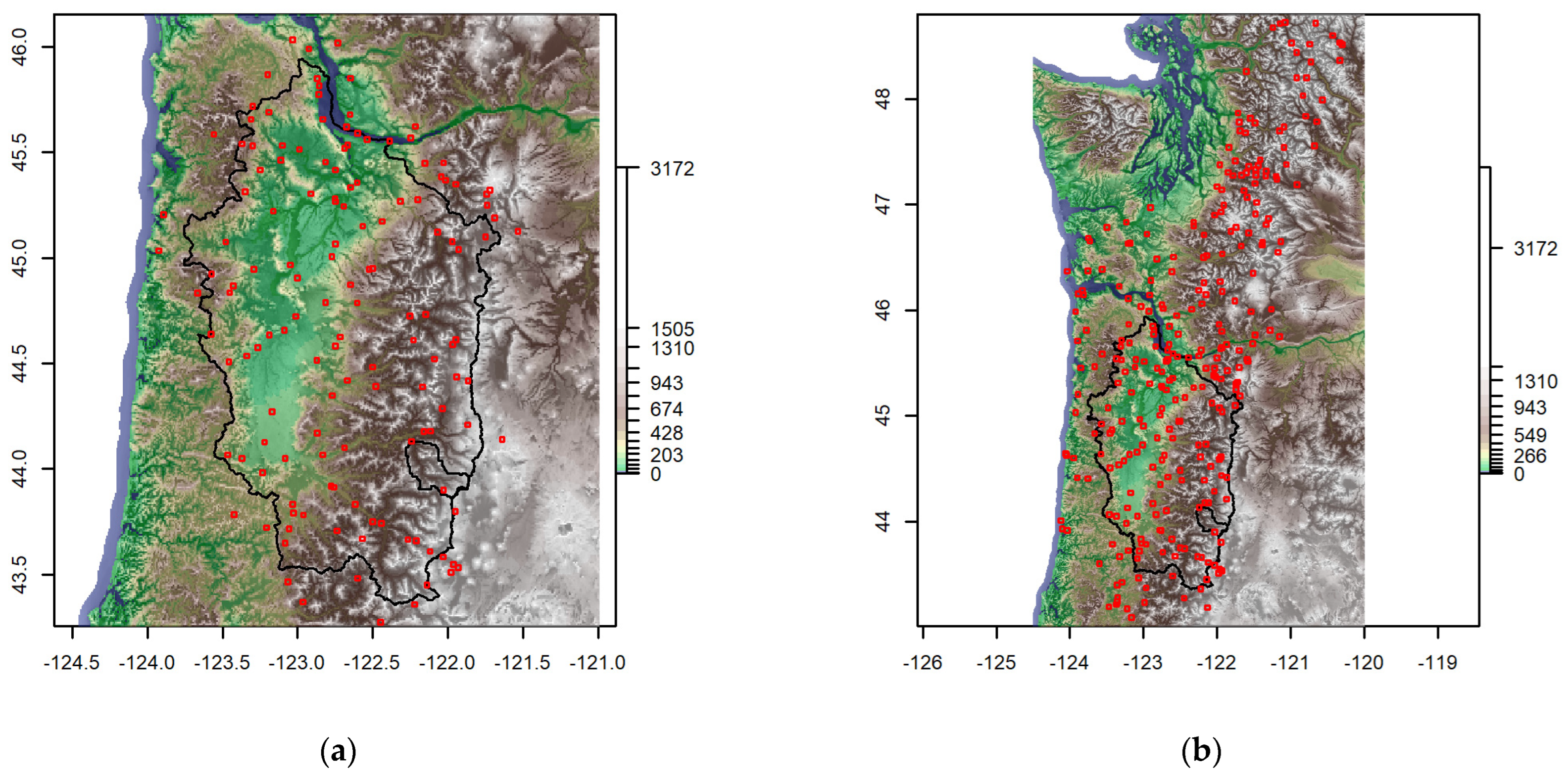
2.4.2. Impact of MSP Areal Exceedance Calculations to Precipitation Gage Extent
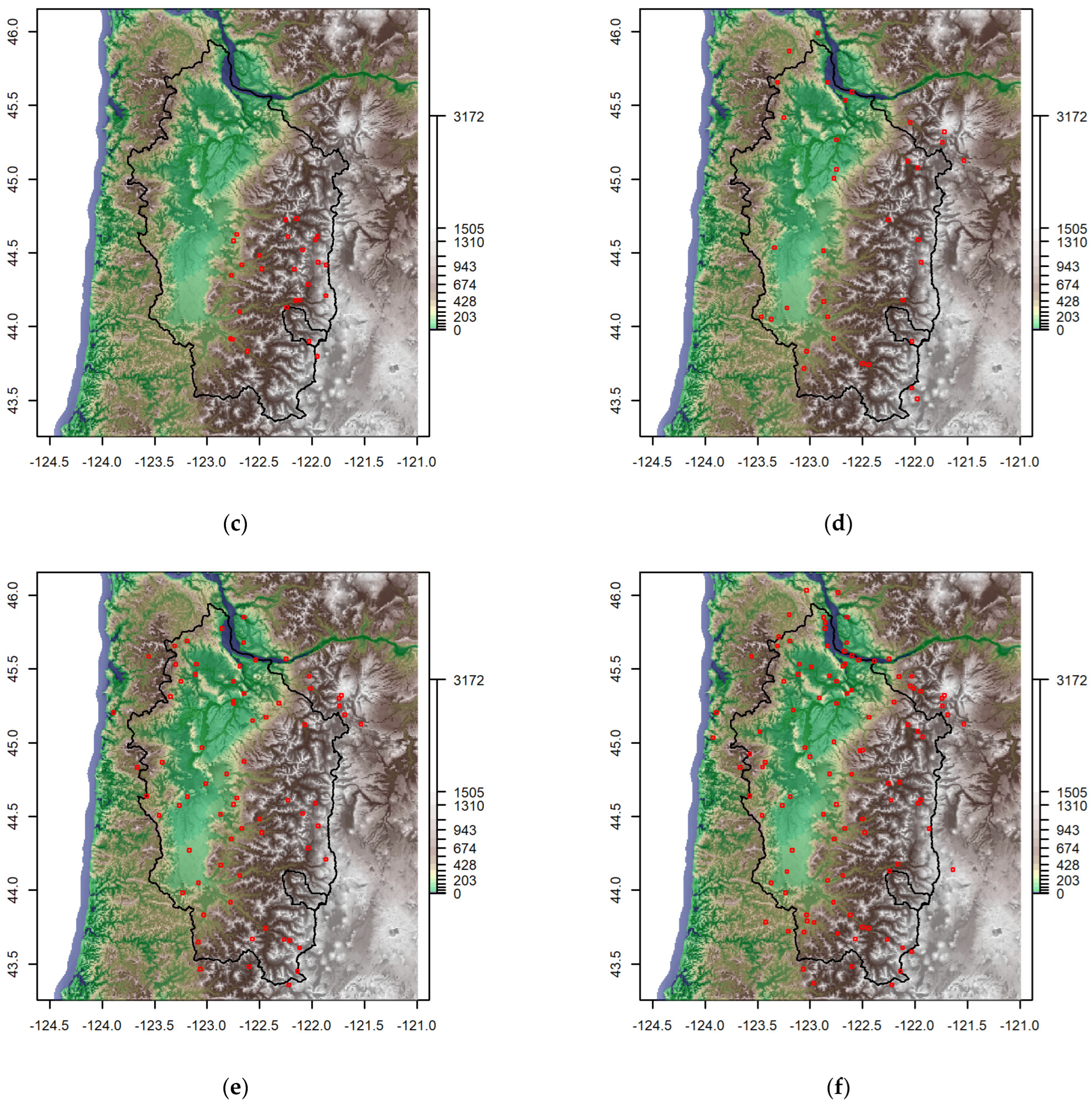
2.4.3. Impact of MSP Areal Exceedance Calculations to Precipitation Gage Density
2.4.4. Impact of MSP Areal Exceedance Calculations on Model Fitting Method
3. Results and Discussion
3.1. Impact of MSP Areal Exceedance Calculations to Study Area Sampling Density
3.2. Impact of MSP Areal Exceedance Calculations to Precipitation Gage Extent
3.3. Impact of MSP Areal Exceedance Calculations to Precipitation Gage Density
3.4. Impact of MSP Areal Exceedance Calculations on Model Fitting Method
4. Conclusions
Author Contributions
Funding
Institutional Review Board Statement
Informed Consent Statement
Data Availability Statement
Acknowledgments
Conflicts of Interest
References
- National Research Council. Estimating Probabilities of Extreme Floods: Methods and Recommended Research; National Academy Press: Washington, DC, USA, 1988. [Google Scholar]
- Subcommittee on Hydrology Extreme Storm Events Work Group. Extreme Rainfall Product Needs; Water Information Coordination Program, Advisory Committee on Water Information, U.S. Geological Survey Washington, D.C. 2018. Available online: https://acwi.gov/hydrology/extreme-storm/product_needs_proposal_20181010.pdf (accessed on 16 May 2023).
- Skahill, B.E.; Viglione, A.; Byrd, A.R. A Bayesian Analysis of the Flood Frequency Hydrology Concept; U.S. Army Engineer Research and Development Center Coastal and Hydraulics Laboratory Technical Note CHETN-X-1: Vicksburg, MS, USA, 2016; Available online: https://hdl.handle.net/11681/21563 (accessed on 16 May 2023).
- Smith, H. Verification of the Bayesian Estimation and Fitting Software (RMC-BestFit); U.S. Army Corps of Engineers Risk Management Center Technical Report RMC-TR-2020-02: Lakewood, CO, USA, 2020; Available online: https://www.iwrlibrary.us/#/document/6f34186c-813c-4fde-85d7-4395988fe607 (accessed on 16 May 2023).
- Smith, H.; Doughty, M. RMC-BestFit Quick Start Guide; U.S. Army Corps of Engineers Risk Management Center Technical Report RMC-TR-2020-03: Lakewood, CO, USA, 2020; Available online: https://www.iwrlibrary.us/#/document/f1767e9f-714d-43b7-cf74-ed1bd65f9dd9 (accessed on 16 May 2023).
- Smith, H.C.; Skahill, B.E. Estimating Design Floods with a Specified Return Period Using Bayesian Analysis. In Proceedings of the New Zealand Society on Large Dams Australian National Committee on Large Dams 2019|Combined Conference, Resilient Dams & Levees for Resilient Communities, Auckland, New Zealand, 9–12 October 2019; Available online: https://www.ancold.org.au/?product=2019-estimating-design-floods-with-a-specified-annual-exceedance-probability-using-bayesian-analysis (accessed on 16 May 2023).
- U.S. Department of the Interior Bureau of Reclamation; U.S. Army Corps of Engineers. Best Practices in Dam and Levee Safety Risk Analysis; U.S. Department of the Interior Bureau of Reclamation: Washington, DC, USA, 2019. Available online: https://www.usbr.gov/damsafety/risk/methodology.html (accessed on 16 May 2023).
- Vasu, N.N.; Lee, S.R.; Pradhan, A.M.S.; Kim, Y.T.; Kang, S.H.; Lee, D.H. A new approach to temporal modelling for landslide hazard assessment using an extreme rainfall induced-landslide index. Eng. Geol. 2016, 215, 36–49. [Google Scholar] [CrossRef]
- Gentilucci, M.; Materazzi, M.; Pambianchi, G. Statistical Analysis of Landslide Susceptibility, Macerata Province (Central Italy). Hydrology 2021, 8, 5. [Google Scholar] [CrossRef]
- Cooley, D.; Cisewski, J.; Erhardt, R.; Jeon, S.; Mannshardt, E.; Omolo, B.; Sun, Y. A Survey of Spatial Extremes: Measuring Spatial Dependence and Modeling Spatial Effects. RevStat 2012, 10, 135–165. [Google Scholar] [CrossRef]
- Davison, A.; Padoan, S.; Ribatet, M. Statistical Modelling of Spatial Extremes. Stat. Sci. 2012, 27, 161–186. [Google Scholar] [CrossRef]
- Ribatet, M. Spatial Extremes: Max-Stable Processes at Work. J. Société Française De Stat. (Spec. Ed. Extrem. Value Theory) 2013, 154, 156–177. Available online: http://www.numdam.org/item/JSFS_2013__154_2_156_0/ (accessed on 16 May 2023).
- Ribatet, M. Modelling Spatial Extremes Using Max-Stable Processes. In Nonlinear and Stochastic Climate Dynamics; Franzke, C., O’Kane, T., Eds.; Cambridge University Press: Cambridge, UK, 2017; pp. 369–391. [Google Scholar] [CrossRef]
- Ribatet, M.; Dombry, C.; Oesting, M. Spatial Extremes and Max-Stable Processes. In Extreme Value Modeling and Risk Analysis: Methods and Applications; Dey, D.K., Yan, J., Eds.; Chapman and Hall/CRC: New York, NY, USA, 2015; Chapter 9. [Google Scholar] [CrossRef]
- Hosking, J.R.M.; Wallis, J.R. Regional Frequency Analysis: An Approach Based on L-Moments; Cambridge University Press: Cambridge, UK, 1997. [Google Scholar]
- Renard, B. A Bayesian hierarchical approach to regional frequency analysis. Water Resour. Res. 2011, 47, W11513. [Google Scholar] [CrossRef]
- Wright, D.B.; Smith, J.A.; Baeck, M.L. Critical Examination of Area Reduction Factors. J. Hydrol. Eng. 2014, 19, 769–776. [Google Scholar] [CrossRef]
- Davison, A.C.; Gholamrezaee, M.M. Geostatistics of extremes. Proc. R. Soc. A 2011, 468, 581–608. [Google Scholar] [CrossRef]
- Azizah, S.; Sutikno, S.; Purhadi, P. Parameter Estimation of Smith Model Max-Stable Process Spatial Extreme Value (Case-Study: Extreme Rainfall Modelling in Ngawi Regency). IPTEK J. Sci. 2017, 2, 16–20. [Google Scholar] [CrossRef]
- Coles, S.G.; Tawn, J.A. Modelling Extremes of the Areal Rainfall Process. J. R. Stat. Society. Ser. B (Methodol.) 1996, 58, 329–347. Available online: https://www.jstor.org/stable/2345980 (accessed on 16 May 2023). [CrossRef]
- Diriba, T.A.; Debusho, L.K. Statistical Modeling of Spatial Extremes through Max-Stable Process Models: Application to Extreme Rainfall Events in South Africa. J. Hydrol. Eng. 2021, 26, 05021028. [Google Scholar] [CrossRef]
- Hakim, A.R.; Sutikno, S.; Prastyo, D.D. Spatial Extreme Value Modeling Using Max-Stable Processes Approach (Case Study: Rainfall intensity in Ngawi). In Proceedings of the 3rd International Conference on Research, Implementation and Education of Mathematics and Science (3rd ICRIEMS), Yogyakarta, Indonesia, 16–17 May 2016. [Google Scholar]
- Jurado, O.E.; Ulrich, J.; Scheibel, M.; Rust, H.W. Evaluating the Performance of a Max-Stable Process for Estimating Intensity-Duration-Frequency Curves. Water 2020, 12, 3314. [Google Scholar] [CrossRef]
- Le, P.D.; Leonard, M.; Westra, S. Modeling Spatial dependence of rainfall extremes across multiple durations. Water Resour. Res. 2018, 54, 2233–2248. [Google Scholar] [CrossRef]
- Neves, M.; Gomes, D.P. Geostatistics for spatial extremes. A case study of maximum annual rainfall in Portugal. Procedia Environ. Sci. 2011, 7, 246–251. [Google Scholar] [CrossRef]
- Olinda, R.A.; Blanchet, J.; dos Santos, C.A.C.; Ozaki, V.A.; Ribeiro, P.J., Jr. Spatial Extremes Modeling Applied to Extreme Precipitation Data in the State of Paraná. Hydrol. Earth Syst. Sci. Discuss 2014, 11, 12731–12764. [Google Scholar] [CrossRef]
- Padoan, S.A.; Ribatet, M.; Sisson, S.A. Likelihood-Based Inference for Max-Stable Processes. J. Am. Stat. Assoc. 2010, 105, 263–277. [Google Scholar] [CrossRef]
- Reich, B.J.; Shaby, B.A. A Hierarchical Max-Stable Spatial Model for Extreme Precipitation. Ann. Appl. Stat. 2012, 6, 1430–1451. [Google Scholar] [CrossRef]
- Saunders, K.; Stephenson, A.G.; Taylor, P.G.; Karoly, D. The spatial distribution of rainfall extremes and the influence of El Niño Southern Oscillation. Weather Clim. Extrem. 2017, 18, 17–28. [Google Scholar] [CrossRef]
- Shang, H.; Yan, J.; Zhang, X. El Niño–Southern Oscillation influence on winter maximum daily precipitation in California in a spatial model. Water Resour. Res. 2011, 47, W11507. [Google Scholar] [CrossRef]
- Stephenson, A.G.; Lehmann, E.A.; Phatak, A. A Max-Stable Process Model for Rainfall Extremes at Different Accumulation Durations. Weather Clim. Extrem. 2016, 13, 44–53. [Google Scholar] [CrossRef]
- Yasin, H.; Hakim, A.R.; Warsito, B.; Santoso, R. Extreme rainfall prediction using spatial extreme value by Max Stable Process (MSP) Smith model approach. J. Phys. Conf. Ser. 2019, 1217, 012110. [Google Scholar] [CrossRef]
- Ribatet, M. Modelling Spatial Extremes with the Spatial Extremes Package. In Proceedings of the 9th International Conference on Extreme Value Analysis: EVA 2015, Ann Arbor, MI, USA, 15–19 June 2015. [Google Scholar]
- Blanchet, J.; Davison, A.C. Spatial Modeling of Extreme Snow Depth. Ann. Appl. Stat. 2011, 5, 1699–1725. [Google Scholar] [CrossRef]
- Cao, Y.; Li, B. Assessing models for estimation and methods for uncertainty quantification for spatial return levels. Environmetrics 2019, 30, e2508. [Google Scholar] [CrossRef]
- Davis, R.A.; Klüppelberg, C.; Steinkohl, C. Statistical inference for max-stable processes in space and time. J. R. Stat. Soc. Ser. B (Stat. Methodol.) 2013, 75, 791–819. Available online: http://www.jstor.org/stable/24772468 (accessed on 16 May 2023). [CrossRef]
- Love, C.A.; Skahill, B.E.; Russell, B.T.; Baggett, J.S.; AghaKouchak, A. An Effective Trend Surface Fitting Framework for Spatial Analysis of Extreme Events. Geophys. Res. Lett. 2022, 49, e2022GL098132. [Google Scholar] [CrossRef]
- Girons Lopez, M.; Wennerström, H.; Nordén, L.-Å.; Seibert, J. Location and density of rain gauges for the estimation of spatial varying precipitation. Geogr. Ann. Ser. A Phys. Geogr. 2015, 97, 167–179. [Google Scholar] [CrossRef]
- Hohmann, C.; Kirchengast, G.; O, S.; Rieger, W.; Foelsche, U. Small Catchment Runoff Sensitivity to Station Density and Spatial Interpolation: Hydrological Modeling of Heavy Rainfall Using a Dense Rain Gauge Network. Water 2021, 13, 1381. [Google Scholar] [CrossRef]
- Blanchet, J. Max-stable processes and annual maximum snow depth. In Proceedings of the 6th International Conference on Extreme Value Analysis, Fort Collins, CO, USA, 23–26 June 2009; Available online: https://www.stat.colostate.edu/graybillconference2009/Presentations/Blanchet.pdf (accessed on 16 May 2023).
- Friedman, J.; Hastie, T.; Tibshirani, R. Regularization Paths for Generalized Linear Models via Coordinate Descent. J. Stat. Softw. 2010, 33, 1–22. [Google Scholar] [CrossRef]
- Tibshirani, R.; Bien, J.; Friedman, J.; Hastie, T.; Simon, N.; Taylor, J.; Tibshirani, R.J. Strong rules for discarding predictors in lasso-type problems. J. R. Stat. Soc. Ser. B Stat. Methodol. 2012, 74, 245–266. [Google Scholar] [CrossRef]
- Simon, N.; Friedman, J.; Hastie, T.; Tibshirani, R. Regularization Paths for Cox’s Proportional Hazards Model via Coordinate Descent. J. Stat. Softw. 2011, 39, 1–13. Available online: https://www.jstatsoft.org/article/view/v039i05 (accessed on 16 May 2023). [CrossRef]
- Ralph, F.M.; Dettinger, M.D. Historical and National Perspectives on Extreme West Coast Precipitation Associated with Atmospheric Rivers during December 2010. Bull. Amer. Meteor. Soc. 2012, 93, 783–790. [Google Scholar] [CrossRef]
- Hu, H.; Dominguez, F.; Wang, Z.; Lavers, D.A.; Zhang, G.; Ralph, F.M. Linking Atmospheric River Hydrological Impacts on the U.S. West Coast to Rossby Wave Breaking. J. Clim. 2017, 30, 3381–3399. [Google Scholar] [CrossRef]
- Hirschboeck, K.K. The role of climate in the generation of floods. In National Water Summary 1988–1989 USGS Water Supply Paper 2375; Paulson, R.W., Chase, E.B., Roberts, R.S., Moody, D.W., Eds.; United States Geological Survey: Denver, CO, USA, 1991. [Google Scholar]
- Curtis, S. Developing a Climatology of the South’s ‘Other’ Storm Season: ENSO Impacts on Winter Extratropical Cyclogenesis. Southeast. Geogr. 2006, 46, 231–244. Available online: https://www.jstor.org/stable/10.2307/26222238 (accessed on 16 May 2023). [CrossRef]
- Senkbeil, J.C.; Brommer, D.M.; Comstock, I.J.; Loyd, T. Hydrometeorological application of an extratropical cyclone classification scheme in the southern United States. Appl Clim. 2012, 109, 27–38. [Google Scholar] [CrossRef]
- Skahill, B.E.; Duren, A.M.; Cunha, L.; Bahner, C. Spatial Analysis of Precipitation and Snow Water Equivalent Extremes for the Columbia River Basin; U.S. Army Engineer Research and Development Center Coastal and Hydraulics Laboratory Technical Report TR-20-10: Vicksburg, MS, USA, 2020. [Google Scholar] [CrossRef]
- Martins, E.S.; Stedinger, J.R. Generalized maximum-likelihood generalized extreme-value quantile estimators for hydrologic data. Water Resour. Res. 2000, 36, 737–744. [Google Scholar] [CrossRef]
- Karlovits, G.S.; Otero, W.; Brown, W.A. Willamette Basin Regional 72-Hour Wintertime Precipitation Frequency Analysis; U.S. Army Corps of Engineers Risk Management Center Technical Report RMC-TR-2017-05: Lakewood, CO, USA, 2017; Available online: https://publibrary.planusace.us/document/1ab0a6a6-9c48-41c8-d984-f57ce9bdb209 (accessed on 16 May 2023).
- Martin, D.L.; Caldwell, R.J.; Parzybok, T.W.; Bahls, V.; Crow, B.R.; Gibson, W. Trinity River Hydrologic Hazards Project Task 2 Report—Storm Typing for the Trinity River Basin; Prepared for: U.S. Army Corps of Engineers; MetStat, Inc.: Fort Collins, CO, USA, 2018. [Google Scholar]
- Martin, D.L.; Schaefer, M.; Parzybok, T.W.; Ward, K.; Bahls, V.; Caldwell, R.J. Regional Extreme Precipitation-Frequency Analysis for the Trinity River Basin; Prepared for: U.S. Army Corps of Engineers; MetStat, Inc.: Fort Collins, CO, USA, 2018. [Google Scholar]
- Daly, C.; Halbleib, M.; Smith, J.I.; Gibson, W.P.; Doggett, M.K.; Taylor, G.H.; Curtis, J.; Pasteris, P.P. Physiographically Sensitive Mapping of Climatological Temperature and Precipitation across the Conterminous United States. Int. J. Climatol. 2008, 28, 2031–2064. [Google Scholar] [CrossRef]
- Javier, J.R.N.; Smith, J.A.; England, J.; Baeck, M.L.; Steiner, M.; Ntelekos, A.A. Climatology of extreme rainfall and flooding from orographic thunderstorm systems in the upper Arkansas River Basin. Water Resour. Res. 2007, 43. [Google Scholar] [CrossRef]
- Oki, T.; Musiake, K.; Koike, T. Spatial rainfall distribution at a storm event in mountainous regions, estimated by orography and wind direction. Water Resour. Res. 1991, 27, 359–369. [Google Scholar] [CrossRef]
- Papalexiou, S.M.; Markonis, Y.; Lombardo, F.; AghaKouchak, A.; Foufoula-Georgiou, E. Precise temporal disaggregation preserving marginals and correlations (DIPMAC) for stationary and nonstationary processes. Water Resour. Res. 2018, 54, 7435–7458. [Google Scholar] [CrossRef]
- Adler, R.F.; Gu, G.; Wang, J.-J.; Huffman, G.J.; Curtis, S.; Bolvin, D. Relationships between global precipitation and surface temperature on interannual and longer timescales (1979–2006). J. Geophys. Res. 2008, 113, D22104. [Google Scholar] [CrossRef]
- Trenberth, K.E.; Shea, D.J. Relationships between precipitation and surface temperature. Geophys. Res. Lett. 2005, 32, L14703. [Google Scholar] [CrossRef]
- Zhao, W.; Khalil, M.A.K. The relationship between precipitation and temperature over the contiguous United States. J. Clim. 1993, 6, 1232–1236. [Google Scholar] [CrossRef]
- De Haan, L. A Spectral Representation for Max-Stable Processes. Ann. Probab. 1984, 12, 1194–1204. [Google Scholar] [CrossRef]
- Opitz, T. Extremal-T Process: Elliptical Domain of Attraction and a Spectral Representation. J. Multivar. Anal. 2013, 122, 409–413. [Google Scholar] [CrossRef]
- Ribatet, M. SpatialExtremes: Modelling Spatial Extremes. R Package Version 2.0-8. 2020. Available online: https://CRAN.R-project.org/package=SpatialExtremes (accessed on 16 May 2023).
- Takeuchi, K. Distribution of Informational Statistics and a Criterion of Fitting. Suri-Kagaku 1976, 153, 12–18. (In Japanese) [Google Scholar]
- Smith, R.L. Max-Stable Processes and Spatial Extremes. Unpublished Manuscript. 1990. Available online: https://www.rls.sites.oasis.unc.edu/postscript/rs/spatex.pdf (accessed on 16 May 2023).
- Brown, B.M.; Resnick, S.I. Extreme Values of Independent Stochastic Processes. J. Appl. Probab. 1977, 14, 732–739. [Google Scholar] [CrossRef]
- Kabluchko, Z.; Schlather, M.; deHaan, L. Stationary Max-Stable Fields Associated to Negative Definite Functions. Ann. Probab. 2009, 37, 2042–2065. [Google Scholar] [CrossRef]
- Nicolet, G.; Eckert, N.; Morin, S.; Blanchet, J. Inferring Spatio-Temporal Patterns in Extreme Snowfall in the French Alps Using Max-stable Processes. Procedia Environ. Sci. 2015, 26, 24–31. [Google Scholar] [CrossRef]
- Schlather, M.; Tawn, J. A Dependence Measure for Multivariate and Spatial Extremes: Properties and Inference. Biometrika 2003, 90, 139–156. Available online: https://www.jstor.org/stable/30042025 (accessed on 16 May 2023). [CrossRef]
- Cooley, D.; Naveau, P.; Poncet, P. Variograms for spatial max-stable random fields. In Dependence in Probability and Statistics; Lecture Notes in Statistics; Bertail, P., Soulier, P., Doukhan, P., Eds.; Springer: New York, NY, USA, 2006; Volume 187. [Google Scholar] [CrossRef]
- Zou, H.; Hastie, T. Regularization and Variable Selection via the Elastic Net. J. R. Stat. Soc. B 2005, 67, 301–320. Available online: https://www.jstor.org/stable/3647580 (accessed on 16 May 2023). [CrossRef]
- Hoerl, A.E.; Kennard, R.W. Ridge Regression: Biased Estimation for Nonorthogonal Problems. Technometrics 1970, 12, 55–67. [Google Scholar] [CrossRef]
- Tikhonov, A.N. On the Stability of Inverse Problems. Dokl. Akad. Nauk. SSSR 1943, 39, 195–198. [Google Scholar]
- Tibshirani, R. Regression Shrinkage and Selection via the Lasso. J. Royal. Statist. Soc. B 1996, 58, 267–288. Available online: https://www.jstor.org/stable/2346178 (accessed on 16 May 2023). [CrossRef]
- Gareth, J.; Witten, D.; Hastie, T.; Tibshirani, R. An Introduction to Statistical Learning: With Applications in R; Springer: New York, NY, USA, 2013. [Google Scholar]
- Economou, T.; Stephenson, D.B.; Ferro, C.A.T. Spatio-temporal modelling of extreme storms. Ann. Appl. Stat. 2014, 8, 2223–2246. [Google Scholar] [CrossRef]
- Schlather, M. Models for Stationary Max-Stable Random Fields. Extremes 2002, 5, 33–44. [Google Scholar] [CrossRef]
- QGIS Development Team. QGIS Geographic Information System. Open Source Geospatial Foundation Project. 2023. Available online: http://qgis.osgeo.org/ (accessed on 16 May 2023).
- Risser, M.D.; Paciorek, C.J.; Wehner, M.F.; O’Brien, T.A.; Collins, W.D. A probabilistic gridded product for daily precipitation extremes over the United States. Clim. Dyn. 2019, 53, 2517–2538. [Google Scholar] [CrossRef]
- Tan, X.; Wu, X.; Liu, B. Global changes in the spatial extents of precipitation extremes. Environ. Res. Lett. 2021, 15, 054017. [Google Scholar] [CrossRef]
- Wehner, M.; Lee, J.; Risser, M.; Ullrich, P.; Gleckler, P.; Collins, W.D. Evaluation of extreme sub-daily precipitation in high-resolution global climate model simulations. Philos. Trans. R. Soc. A 2021, 379, 20190545. [Google Scholar] [CrossRef]
- Bechler, A.; Vrac, M.; Bel, L. A spatial hybrid approach for downscaling of extreme precipitation fields. J. Geophys. Res. Atmos. 2015, 120, 4534–4550. [Google Scholar] [CrossRef]
- National Weather Service Office of Water Prediction. Analysis of Impact of Nonstationary Climate on NOAA Atlas 14 Estimates; Office of Water Prediction, National Oceanic and Atmospheric Administration: Washington, DC, USA, 2022. [Google Scholar]
- Nash, J.E.; Sutcliffe, J.V. River flow forecasting through conceptual models part I—A discussion of principles. J. Hydrol. 1970, 10, 282–290. [Google Scholar] [CrossRef]
- Gupta, H.V.; Kling, H.; Yilmaz, K.K.; Martinez, G.F. Decomposition of the mean squared error and NSE performance criteria: Implications for improving hydrological modelling. J. Hydrol. 2009, 377, 80–91. [Google Scholar] [CrossRef]
- Tye, M.R.; Cooley, D. A spatial model to examine rainfall extremes in Colorado’s Front Range. J. Hydrol. 2015, 530, 15–23. [Google Scholar] [CrossRef]
- Doherty, J.; Skahill, B.E. An advanced regularization methodology for use in watershed model calibration. J. Hydrol. 2006, 327, 564–577. [Google Scholar] [CrossRef]


| Model Name | MSP Model Description | |
|---|---|---|
| Dataset | ||
| WRB MSP Models | ||
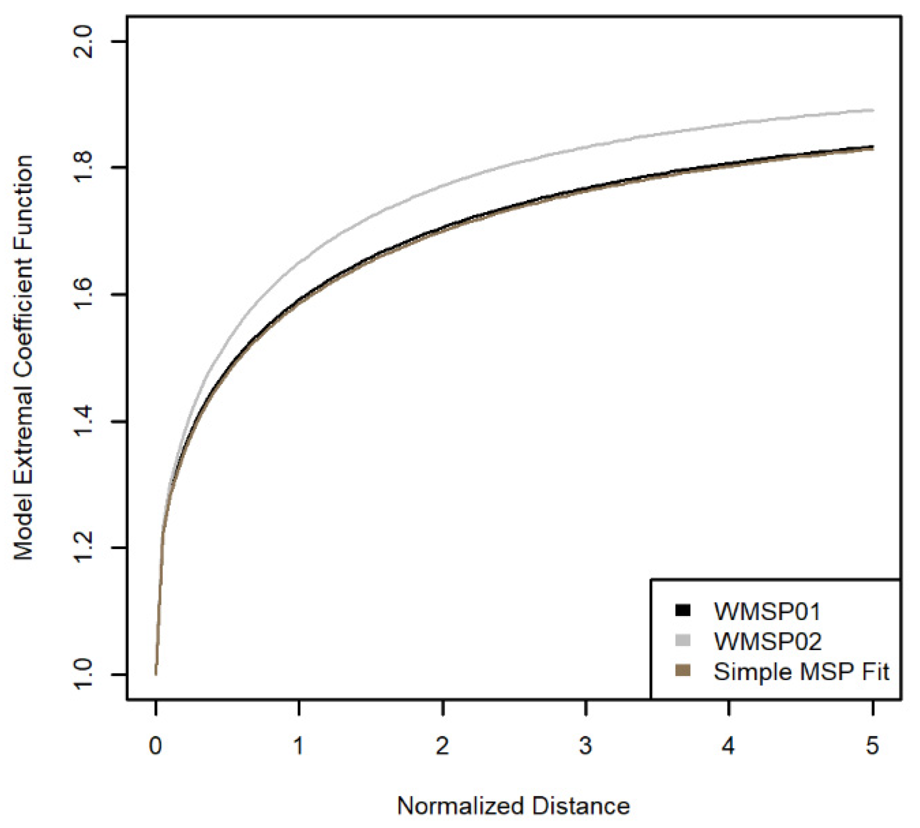
| WMSP01 | Figure 3a | General MSP was fit using constrained optimization and initialized with simple MSP and spatial GEV trend surface parameter estimates |
| WMSP02 | Figure 3a | General MSP was fit using unconstrained optimization and initialized with simple MSP and spatial GEV trend surface parameter estimates |
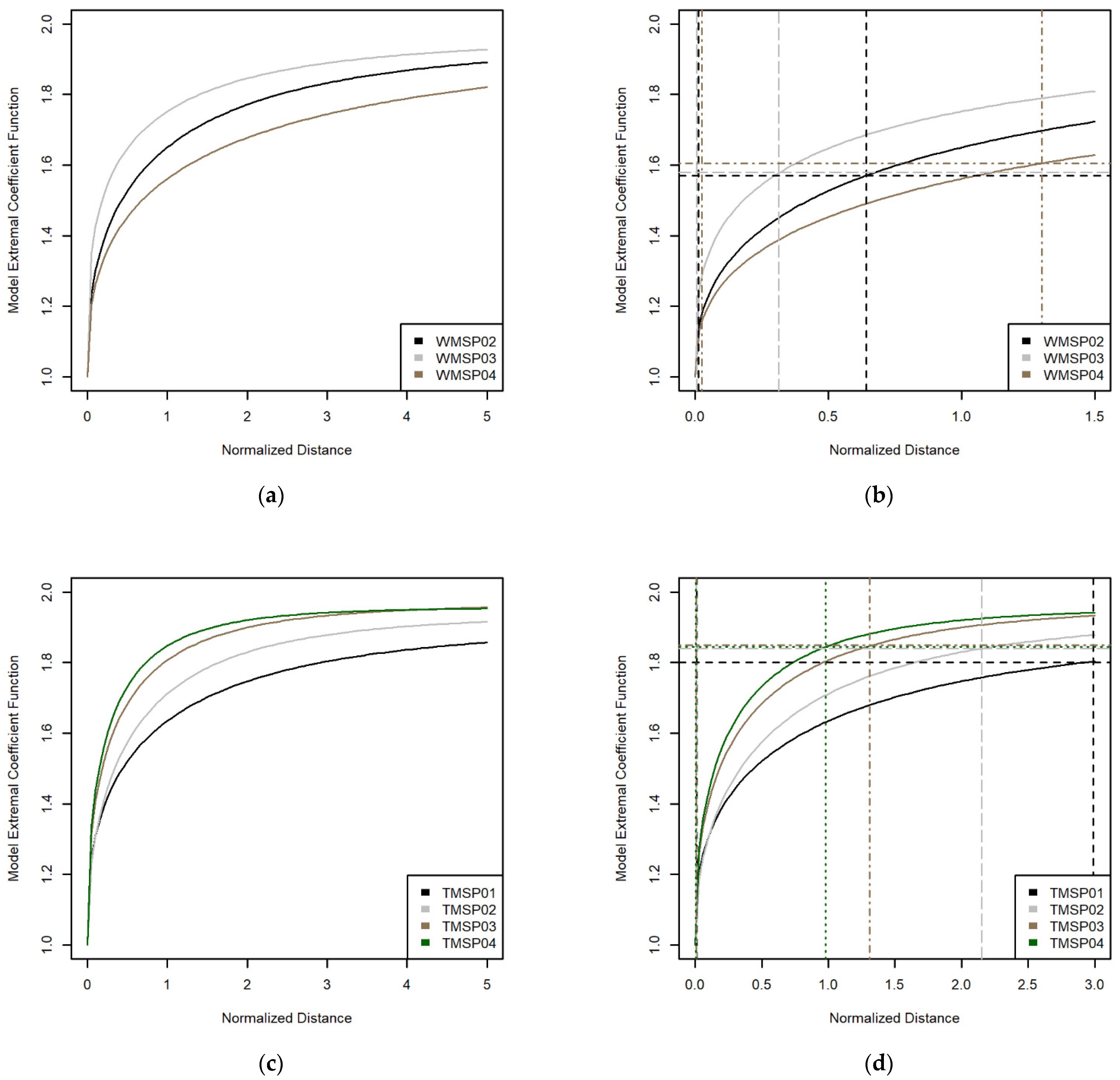
| WMSP03 | Figure 3b | |
| WMSP04 | Figure 3c | |
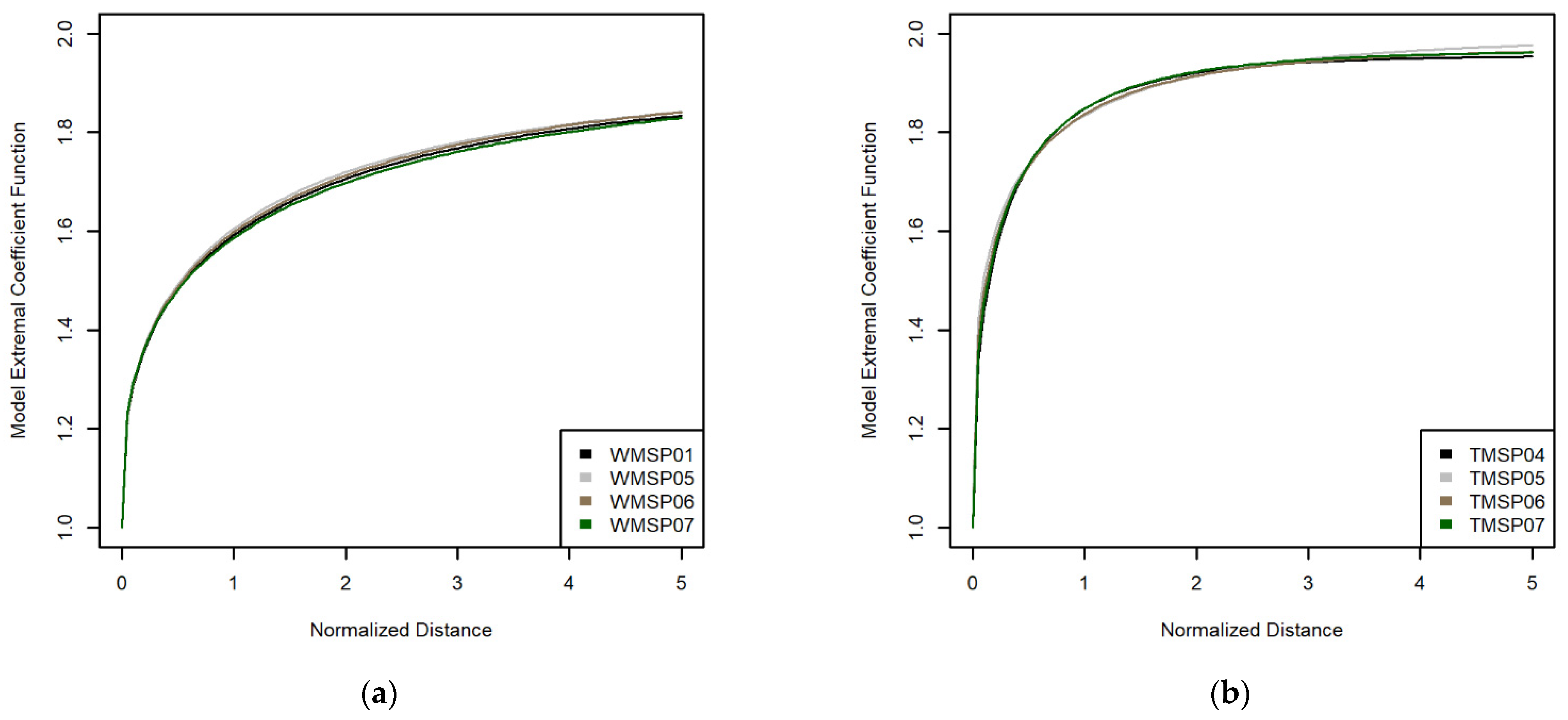
| WMSP05 | Figure 3d | General MSP was fit using constrained optimization and initialized with simple MSP and spatial GEV trend surface parameter estimates |
| WMSP06 | Figure 3e | |
| WMSP07 | Figure 3f | |
| TRB MSP Models | ||
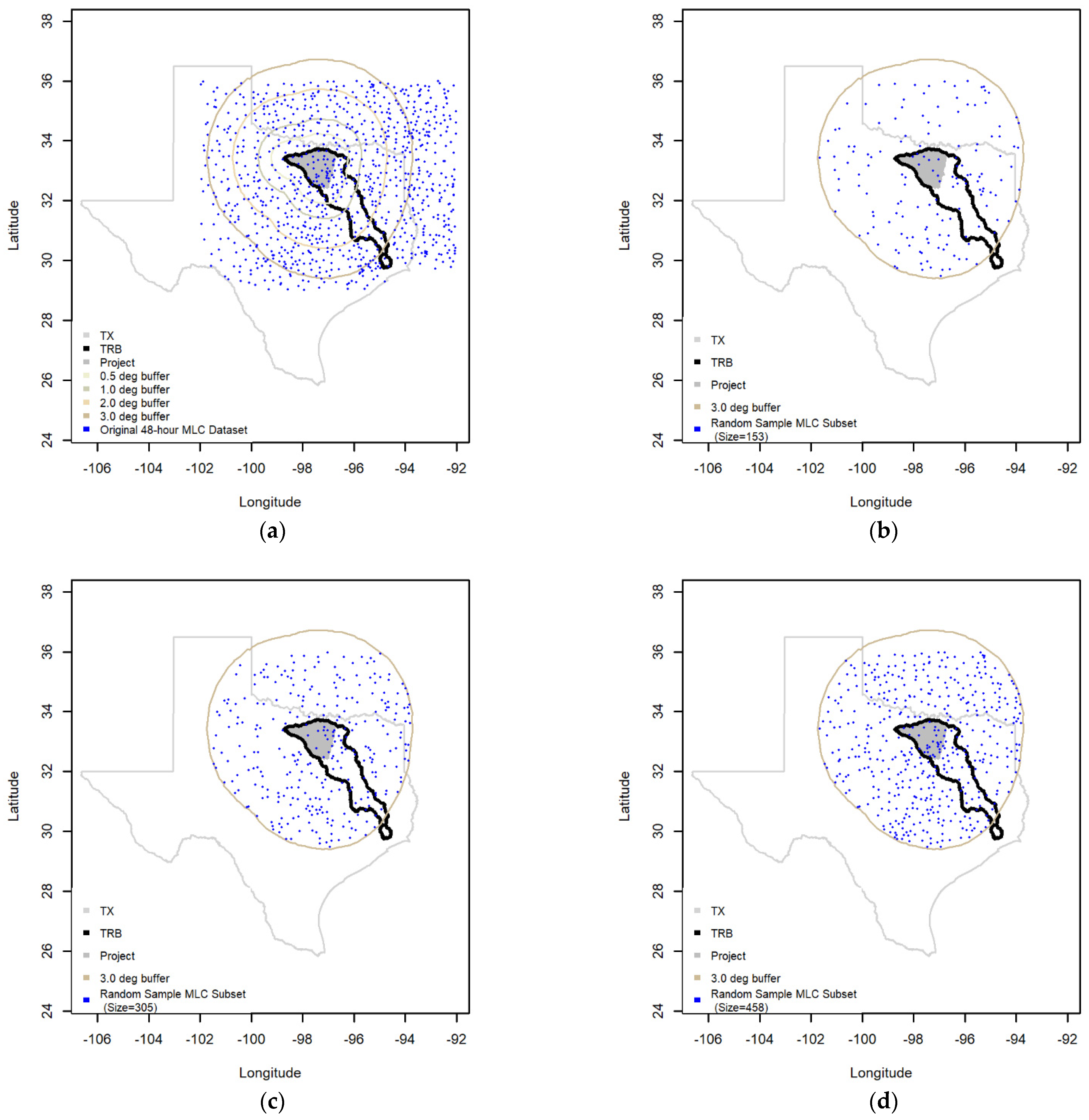
| TMSP01 | Figure 4a | Used the 85 precipitation gages within the 0.5° buffer of the project area |
| TMSP02 | Figure 4a | Used the 151 precipitation gages within the 1° buffer of the project area |
| TMSP03 | Figure 4a | Used the 360 precipitation gages within the 2° buffer of the project area |
| TMSP04 | Figure 4a | Used the 610 precipitation gages within the 3° buffer of the project area |
| TMSP05 | Figure 4b | A random sample of 153 (~25%) of the 610 precipitation gages within the 3° buffer of the project area |
| TMSP06 | Figure 4c | A random sample of 305 (50%) of the 610 precipitation gages within the 3° buffer of the project area |
| TMSP07 | Figure 4d | A random sample of 458 (~75%) of the 610 precipitation gages within the 3° buffer of the project area |
| AEP | |||||
|---|---|---|---|---|---|
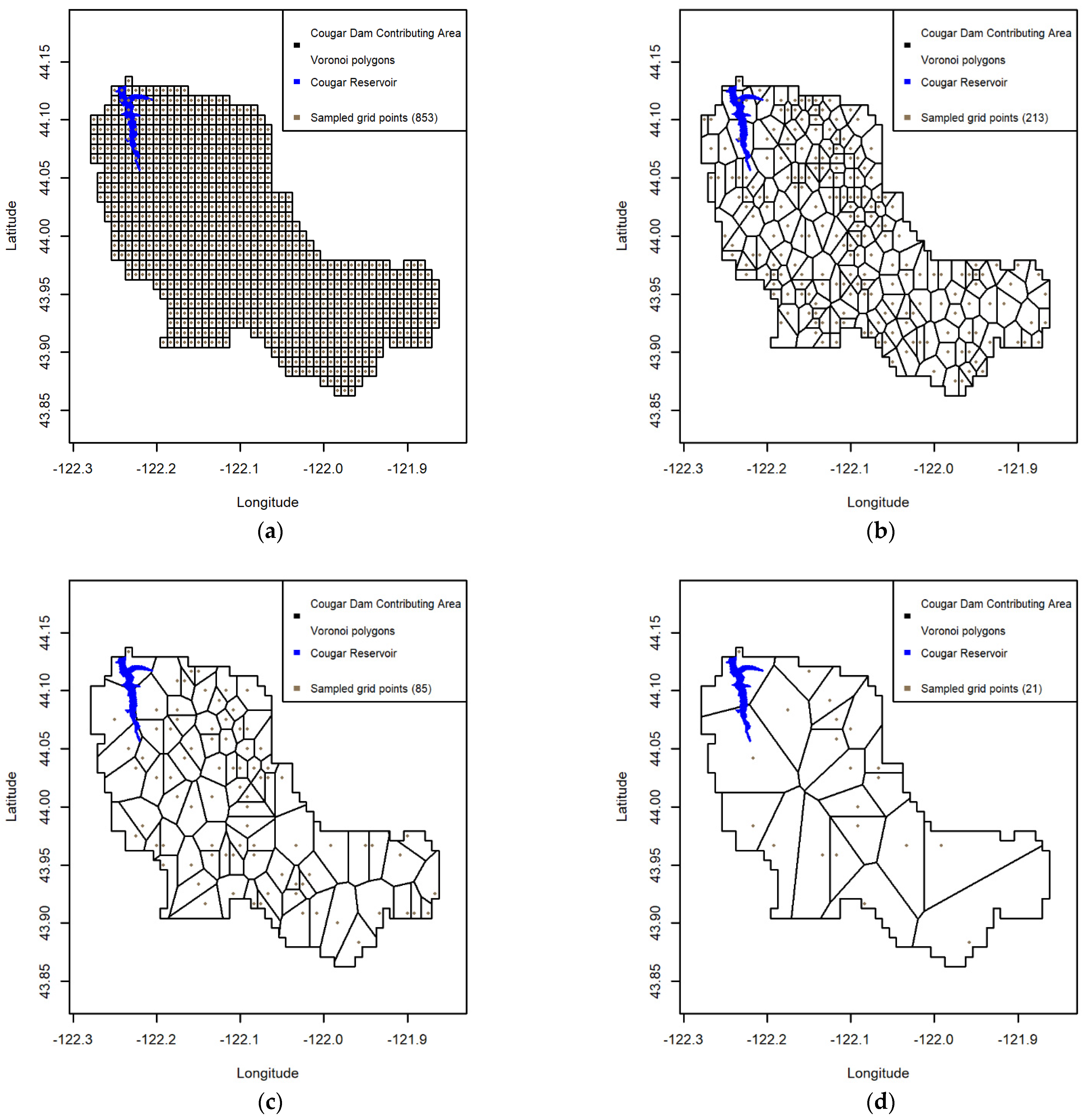
| Sampling Density | 10−1 | 10−2 | 10−3 | 10−4 | |
| 100% (853 points) | 1 | 9.71 | 13.47 | 17.50 | 21.55 |
| 25% (213 points) | 2 | 9.74 | 13.44 | 17.22 | 21.23 |
| 3 | 9.74 (9.72, 9.78) | 13.44 (13.35, 13.52) | 17.21 (16.95, 17.52) | 21.27 (20.01, 21.81) | |
| 4 | 9.73 (9.72, 9.76) | 13.44 (13.34, 13.51) | 17.22 (16.95, 17.55) | 21.20 (20.06, 21.96) | |
| 10% (85 points) | 5 | 9.69 | 13.41 | 17.27 | 21.27 |
| 6 | 9.69 (9.67, 9.72) | 13.41 (13.34, 13.53) | 17.27 (17.03, 17.62) | 21.34 (20.42, 22.08) | |
| 7 | 9.68 (9.65, 9.70) | 13.39 (13.33, 13.50) | 17.22 (17.03, 17.51) | 21.16 (20.20, 21.75) | |
| 2.5% (21 points) | 8 | 9.77 | 13.49 | 17.30 | 21.45 |
| 9 | 9.77 (9.75, 9.80) | 13.50 (13.43, 13.60) | 17.30 (17.09, 17.55) | 21.49 (20.82, 22.61) | |
| 10 | 9.74 (9.71, 9.76) | 13.45 (13.39, 13.54) | 17.26 (16.98, 17.59) | 21.48 (20.55, 22.60) | |
| Probability | |||||||||||||
|---|---|---|---|---|---|---|---|---|---|---|---|---|---|
| Study Area Sampling Density | 0.01 | 0.1 | 0.2 | 0.3 | 0.4 | 0.5 | 0.6 | 0.7 | 0.8 | 0.9 | 0.99 | SSD | |
| 100% | 1 | 14.70 | 14.94 | 15.43 | 15.97 | 16.64 | 17.50 | 18.38 | 19.34 | 20.19 | 20.96 | 22.35 | |
| 25% | 2 | 14.71 | 14.98 | 15.46 | 16.18 | 16.99 | 17.96 | 18.99 | 19.67 | 20.41 | 21.07 | 22.41 | 0.94 |
| 3 | 14.75 | 14.96 | 15.45 | 15.96 | 16.64 | 17.44 | 18.44 | 19.28 | 20.20 | 20.99 | 22.34 | 0.015 | |
| 10% | 4 | 14.74 | 14.98 | 15.46 | 16.54 | 17.38 | 18.18 | 19.14 | 19.72 | 20.62 | 20.98 | 22.23 | 2.26 |
| 5 | 14.70 | 15.01 | 15.45 | 16.01 | 16.69 | 17.52 | 18.47 | 19.35 | 20.16 | 21.00 | 22.26 | 0.028 | |
| 2.5% | 6 | 15.17 | 15.45 | 16.20 | 17.01 | 17.63 | 19.04 | 19.64 | 20.22 | 21.01 | 21.53 | 22.13 | 8.91 |
| 7 | 14.75 | 14.95 | 15.46 | 16.19 | 16.89 | 17.63 | 18.42 | 19.30 | 20.11 | 21.05 | 22.42 | 0.156 | |
| Areal Means | |||||
|---|---|---|---|---|---|
| Sampling Density | 1 | 2 | 3 | 4 | 5 |
| 100% | 3.61 | 2.69 | 3.56 | 2.99 | 2.57 |
| 10% | 3.60 | 2.68 | 3.54 | 2.99 | 2.57 |
| 1% | 3.59 | 2.66 | 3.63 | 3.00 | 2.59 |
| AEP | ||||
|---|---|---|---|---|
| Gage Extent (Model) | 10−1 | 10−2 | 10−3 | 10−4 |
| WMSP02 | 9.66 | 13.49 | 17.55 | 22.03 |
| WMSP03 | 9.54 | 13.48 | 17.83 | 22.42 |
| WMSP04 | 9.53 | 13.33 | 17.4 | 21.54 |
| AEP | ||||
|---|---|---|---|---|
| Gage Extent (Model) | 10−1 | 10−2 | 10−3 | 10−4 |
| TMSP01 | 5.06 | 8.23 | 12.83 | 19.81 |
| TMSP02 | 5.06 | 8.20 | 12.90 | 20.21 |
| TMSP03 | 4.95 | 7.88 | 12.16 | 17.77 |
| TMSP04 | 4.84 | 7.71 | 11.88 | 17.33 |
| GEV Location | GEV Scale | Return Levels | |||||||
|---|---|---|---|---|---|---|---|---|---|
| 02/03 | 02/04 | 03/04 | 02/03 | 02/04 | 03/04 | 02/03 | 02/04 | 03/04 | |
| R2 | 1.00 | 0.99 | 0.99 | 0.93 | 0.97 | 0.81 | 0.97 | 0.98 | 0.92 |
| NSE | 0.92 | 0.98 | 0.97 | 0.91 | 0.89 | 0.78 | 0.95 | 0.96 | 0.86 |
| KGE | 0.78 | 0.96 | 0.85 | 0.96 | 0.74 | 0.71 | 0.92 | 0.87 | 0.80 |
| GEV Location | GEV Scale | Return Levels | |||||||||||||
|---|---|---|---|---|---|---|---|---|---|---|---|---|---|---|---|
| 01/02 | 01/03 | 01/04 | 02/04 | 03/04 | 01/02 | 01/03 | 01/04 | 02/04 | 03/04 | 01/02 | 01/03 | 01/04 | 02/04 | 03/04 | |
| R2 | 0.98 | 0.98 | 0.98 | 0.99 | 1.00 | 0.99 | 0.92 | 0.85 | 0.88 | 0.85 | 0.99 | 0.94 | 0.89 | 0.93 | 0.90 |
| NSE | 0.96 | 0.97 | 0.83 | 0.72 | 0.85 | 0.93 | 0.81 | −2.18 | −1.01 | −0.87 | 0.98 | −1.75 | −5.92 | −5.53 | 0.62 |
| KGE | 0.94 | 0.91 | 0.83 | 0.89 | 0.93 | 0.86 | 0.81 | 0.29 | 0.50 | 0.55 | 0.88 | 0.73 | 0.34 | 0.51 | 0.68 |
| GEV Shape Parameter | ||
|---|---|---|
| Model Name | Fitted Value | Standard Error |
| WMSP02 | 0.02496 | 0.004246 |
| WMSP03 | 0.03027 | 0.003833 |
| WMSP04 | 0.01533 | 0.006999 |
| TMSP01 | 0.1441 | 0.009562 |
| TMSP02 | 0.146 | 0.007281 |
| TMSP03 | 0.1233 | 0.004677 |
| TMSP04 | 0.1306 | 0.003947 |
| AEP | ||||
|---|---|---|---|---|
| Gage Extent (Model) | 10−1 | 10−2 | 10−3 | 10−4 |
| WMSP01 | 9.74 | 13.44 | 17.22 | 21.23 |
| WMSP05 | 9.64 | 13.73 | 18.26 | 23.35 |
| WMSP06 | 9.55 | 13.35 | 17.40 | 22.01 |
| WMSP07 | 9.70 | 13.47 | 17.36 | 21.06 |
| AEP | ||||
|---|---|---|---|---|
| Gage Extent (Model) | 10−1 | 10−2 | 10−3 | 10−4 |
| TMSP04 | 4.84 | 7.71 | 11.88 | 17.33 |
| TMSP05 | 4.87 | 7.83 | 12.22 | 18.33 |
| TMSP06 | 4.91 | 7.89 | 12.35 | 18.74 |
| TMSP07 | 4.85 | 7.73 | 11.85 | 17.24 |
| GEV Location | GEV Scale | Return Levels | |||||||||||||
|---|---|---|---|---|---|---|---|---|---|---|---|---|---|---|---|
| 01/05 | 01/06 | 01/07 | 05/07 | 06/07 | 01/05 | 01/06 | 01/07 | 05/07 | 06/07 | 01/05 | 01/06 | 01/07 | 05/07 | 06/07 | |
| R2 | 0.94 | 1.00 | 1.00 | 0.93 | 1.00 | 0.98 | 0.99 | 0.99 | 0.99 | 1.00 | 0.96 | 1.00 | 1.00 | 0.98 | 1.00 |
| NSE | 0.64 | 0.96 | 0.91 | 0.91 | 0.99 | 0.84 | 0.81 | 0.90 | 0.81 | 0.49 | 0.43 | 0.99 | 0.99 | 0.70 | 0.99 |
| KGE | 0.57 | 0.84 | 0.76 | 0.87 | 0.93 | 0.63 | 0.95 | 0.95 | 0.70 | 0.92 | 0.68 | 0.98 | 0.92 | 0.81 | 0.94 |
| GEV Location | GEV Scale | Return Levels | |||||||||||||
|---|---|---|---|---|---|---|---|---|---|---|---|---|---|---|---|
| 04/05 | 04/06 | 04/07 | 05/07 | 06/07 | 04/05 | 04/06 | 04/07 | 05/07 | 06/07 | 04/05 | 04/06 | 04/07 | 05/07 | 06/07 | |
| R2 | 0.91 | 0.98 | 1.00 | 0.94 | 0.99 | 0.91 | 0.95 | 0.97 | 0.90 | 0.98 | 0.96 | 0.96 | 0.98 | 0.96 | 0.99 |
| NSE | 0.85 | 0.95 | 0.99 | 0.85 | 0.97 | 0.72 | 0.61 | 0.86 | 0.88 | 0.86 | 0.77 | 0.37 | 0.97 | 0.82 | 0.21 |
| KGE | 0.82 | 0.91 | 0.96 | 0.83 | 0.94 | 0.90 | 0.75 | 0.87 | 0.80 | 0.83 | 0.97 | 0.76 | 0.90 | 0.88 | 0.82 |
| GEV Shape Parameter | ||
|---|---|---|
| Model Name | Fitted Value | Standard Error |
| WMSP01 | 0.008987 | 0.004033 |
| WMSP05 | 0.04064 | 0.006227 |
| WMSP06 | 0.03001 | 0.004287 |
| WMSP07 | 0.005042 | 0.004189 |
| TMSP04 | 0.1306 | 0.003947 |
| TMSP05 | 0.1315 | 0.004215 |
| TMSP06 | 0.1349 | 0.004135 |
| TMSP07 | 0.1273 | 0.003911 |
| Model Name | Model Fitting Method | GEV Shape Parameter | |
|---|---|---|---|
| Initial Estimate | Final Estimate | ||
| WMSP01 | C | 0.006785831 | 0.008987 |
| WMSP02 | U | 0.006785831 | 0.02496 |
| WMSP03 | U | 0.02036444 | 0.03027 |
| WMSP04 | U | −0.00153159 | 0.01533 |
| WMSP05 | C | 0.03778892 | 0.04064 |
| WMSP06 | C | 0.02769452 | 0.03001 |
| WMSP07 | C | 0.00277155 | 0.005042 |
| TMSP01 | U | 0.1138974 | 0.1441 |
| TMSP02 | U | 0.1246995 | 0.146 |
| TMSP03 | U | 0.1091662 | 0.1233 |
| TMSP04 | U | 0.117473 | 0.1306 |
| TMSP05 | U | 0.1192562 | 0.1315 |
| TMSP06 | U | 0.1201912 | 0.1349 |
| TMSP07 | U | 0.1155369 | 0.1273 |
Disclaimer/Publisher’s Note: The statements, opinions and data contained in all publications are solely those of the individual author(s) and contributor(s) and not of MDPI and/or the editor(s). MDPI and/or the editor(s) disclaim responsibility for any injury to people or property resulting from any ideas, methods, instructions or products referred to in the content. |
© 2023 by the authors. Licensee MDPI, Basel, Switzerland. This article is an open access article distributed under the terms and conditions of the Creative Commons Attribution (CC BY) license (https://creativecommons.org/licenses/by/4.0/).
Share and Cite
Skahill, B.; Smith, C.H.; Russell, B.T.; England, J.F. Impacts of Max-Stable Process Areal Exceedance Calculations to Study Area Sampling Density, Surface Network Precipitation Gage Extent and Density, and Model Fitting Method. Hydrology 2023, 10, 121. https://doi.org/10.3390/hydrology10060121
Skahill B, Smith CH, Russell BT, England JF. Impacts of Max-Stable Process Areal Exceedance Calculations to Study Area Sampling Density, Surface Network Precipitation Gage Extent and Density, and Model Fitting Method. Hydrology. 2023; 10(6):121. https://doi.org/10.3390/hydrology10060121
Chicago/Turabian StyleSkahill, Brian, Cole Haden Smith, Brook T. Russell, and John F. England. 2023. "Impacts of Max-Stable Process Areal Exceedance Calculations to Study Area Sampling Density, Surface Network Precipitation Gage Extent and Density, and Model Fitting Method" Hydrology 10, no. 6: 121. https://doi.org/10.3390/hydrology10060121