Article

Development of Multi-Inflow Prediction Ensemble Model Based on Auto-Sklearn Using Combined Approach: Case Study of Soyang River Dam

1
Agriculture and Life Sciences Research Institute, Kangwon National University, Chuncheon-si 24341, Gangwon-do, Republic of Korea
2
Department of Regional Infrastructure Engineering, Kangwon National University, Chuncheon-si 24341, Gangwon-do, Republic of Korea
3
ILEM Research Institute, Kangwon National University, Chuncheon-si 24341, Gangwon-do, Republic of Korea
4
Department of Agricultural and Biological Engineering, Purdue University, West Lafayette, IN 47907, USA
5
Department of Earth and Environment, Boston University, Boston, MA 02215, USA
*
Author to whom correspondence should be addressed.
Hydrology 2023, 10(4), 90; https://doi.org/10.3390/hydrology10040090
Submission received: 31 March 2023 / Accepted: 6 April 2023 / Published: 11 April 2023
(This article belongs to the Section Water Resources and Risk Management)

Abstract

:
Accurate prediction of dam inflows is essential for effective water resource management and dam operation. In this study, we developed a multi-inflow prediction ensemble (MPE) model for dam inflow prediction using auto-sklearn (AS). The MPE model is designed to combine ensemble models for high and low inflow prediction and improve dam inflow prediction accuracy. We investigated the impact of datasets assigned to flow regimes on the ensemble composition and compared the performance of the MPE model to an AS-based ensemble model developed using a conventional approach. Our findings showed that the MPE model outperformed the conventional model in predicting dam inflows during flood and nonflood periods, reducing the root mean square error (RMSE) and mean absolute error (MAE) by 22.1% and 24.9% for low inflows, and increasing the coefficient of determination (R2) and Nash–Sutcliffe efficiency (NSE) by 21.9% and 35.8%, respectively. These results suggest that the MPE model has the potential to improve water resource management and dam operation, benefiting both the environment and society. Overall, the methodology of this study is expected to contribute to the development of a robust ensemble model for dam inflow prediction in regions with high climate variability.

1. Introduction

The real-time management of water resources in arid and semiarid regions is facing a significant challenge due to the frequent occurrence of floods and droughts caused by climate change [1,2,3]. To address these challenges, many countries have constructed and operated multipurpose dams to stabilize the water supply and control floods [4]. However, the increased variability in the inflow to dams due to changes in climate and land use directly impacts the water level calculation and dam operation [5]. This can cause significant downstream damage from uncontrolled discharge during flood seasons, and make it difficult to ensure the minimum water supplies essential for water quality and aquatic environments during dry seasons [6]. Hence, accurate prediction of dam inflow is critical for effective water resource management and dam operations.
There are two major approaches to modeling studies for dam (or reservoir) inflow prediction: physical or conceptual models [7,8,9,10,11] and data-driven machine learning (ML) models [12,13,14,15,16]. Physical models are effective in simulating hydrologic processes but require in-depth knowledge and calibration [17], while conceptual models have lower data requirements and computational complexity but may be limited by the lack of detailed physical information. Recently, ML models have become more popular for dam inflow prediction due to their simplicity, low data requirements, and robustness [18]. ML models can quickly capture the complexity of dam inflow time-series data without extensive prior knowledge [19]. In addition, many studies have successfully utilized ensemble methods to improve the accuracy of dam inflow predictions [20,21,22,23]. Ensemble modeling is a process in which an ML model combines the predictive capabilities of individual base models unique to the model to generate generalized predictions, allowing for capturing various aspects of the data and providing high prediction performance. However, developing effective ensembles requires a deep understanding of model selection, combination, and hyperparameter optimization. These tasks are often laborious and time-consuming, and there is a risk of human error that can affect the reliability and validity of model predictions.
Automated machine learning (AutoML) can be used as an alternative for developing ensemble models. AutoML can automatically generate various ML models and effectively create an ensemble model by combining them to perform more accurate predictions [24]. It can reduce the risk of human error and increase the reliability of the ensemble model’s predicted values. Its greatest advantage is that it helps save time and effort in selecting ML models and optimizing them without requiring specialized domain knowledge. According to several studies, AutoML can effectively generate satisfactory results for various types of datasets [25,26,27,28]. Despite the success of AutoML in generating satisfactory results for various types of datasets, its performance in dam inflow prediction has not been evaluated.
The dam inflow is greatly influenced by various factors such as precipitation, vegetation, soil, and human activities. In particular, the pattern of dam inflow in regions with high climate variability can show significant differences between rainy and nonrainy seasons [29]. The complex and nonlinear characteristics of data can affect not only the data preprocessing methods of AutoML but also the selection of ensemble models and hyperparameter combinations. Therefore, the development of ensemble models that consider the characteristics of the flow regime is necessary for the accurate prediction of dam inflow. Hong et al. [30] showed that an ensemble of ML models that consider the characteristics of high and low inflow data can improve the limitations of flow regime and rainfall on inflow prediction compared to using a single ML model. Moon et al. [31] developed a flow regime-based ANFIS dam inflow prediction (FADIP) model, which is based on the adaptive neuro-fuzzy inference system (ANFIS), and compared it with an ANFIS dam inflow prediction (ADIP) model. Their results showed that FADIP outperformed ADIP in accuracy throughout the entire period, especially in predicting dam inflow during the normal and low flow seasons. Furthermore, appropriate dataset construction for hydrological flow regimes can alleviate the issue of data imbalance and prediction model generalization by contributing to the learning of various aspects of the data. Zhang et al. [32] demonstrated that a multiclass dataset construction for dam inflow strategies according to different flow regimes can effectively handle high-dimensional data and improve the overall prediction accuracy of ensemble models. Choi et al. [33] demonstrated that applying seasonal division and normalization to dam inflow training data can contribute to reducing errors caused by data deviation and improving the learning accuracy of the multilayer perceptron (MLP) model. However, the impact of datasets assigned to flow regimes on the ensemble composition based on AutoML for dam inflow prediction and its effect on improving ensemble model performance have not been quantified.
Therefore, this study aims to evaluate the performance of an automated machine learning (AutoML) approach for developing a multi-inflow prediction ensemble (MPE) model for dam inflow prediction, which has not been previously evaluated in previous studies. The novelty of this study is that the MPE model trains independent ensemble models for high and low inflow prediction based on auto-sklearn (AS) and combines their predictions, taking into account the characteristics of the hydrological flow regime.
The hypothesis is that the MPE model combining the AS-based approach outperforms the conventional AS-based ensemble model by effectively capturing the complex and nonlinear characteristics of dam inflow time-series data in both flood and nonflood periods.
The main objectives of this study are to develop the MPE model, evaluate its performance by comparing it to a conventional AS-based ensemble model, quantify the impact of datasets assigned to flow regimes on the ensemble composition based on AutoML and provide insight into developing an AS-based robust ensemble model for predicting dam inflow. The methodology of this study is expected to contribute to sustainable water resource management and dam operations in regions with high climate variability.

2. Materials and Methods

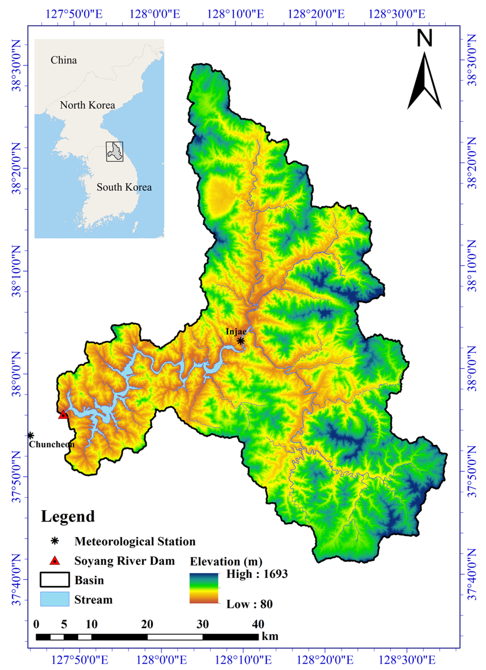
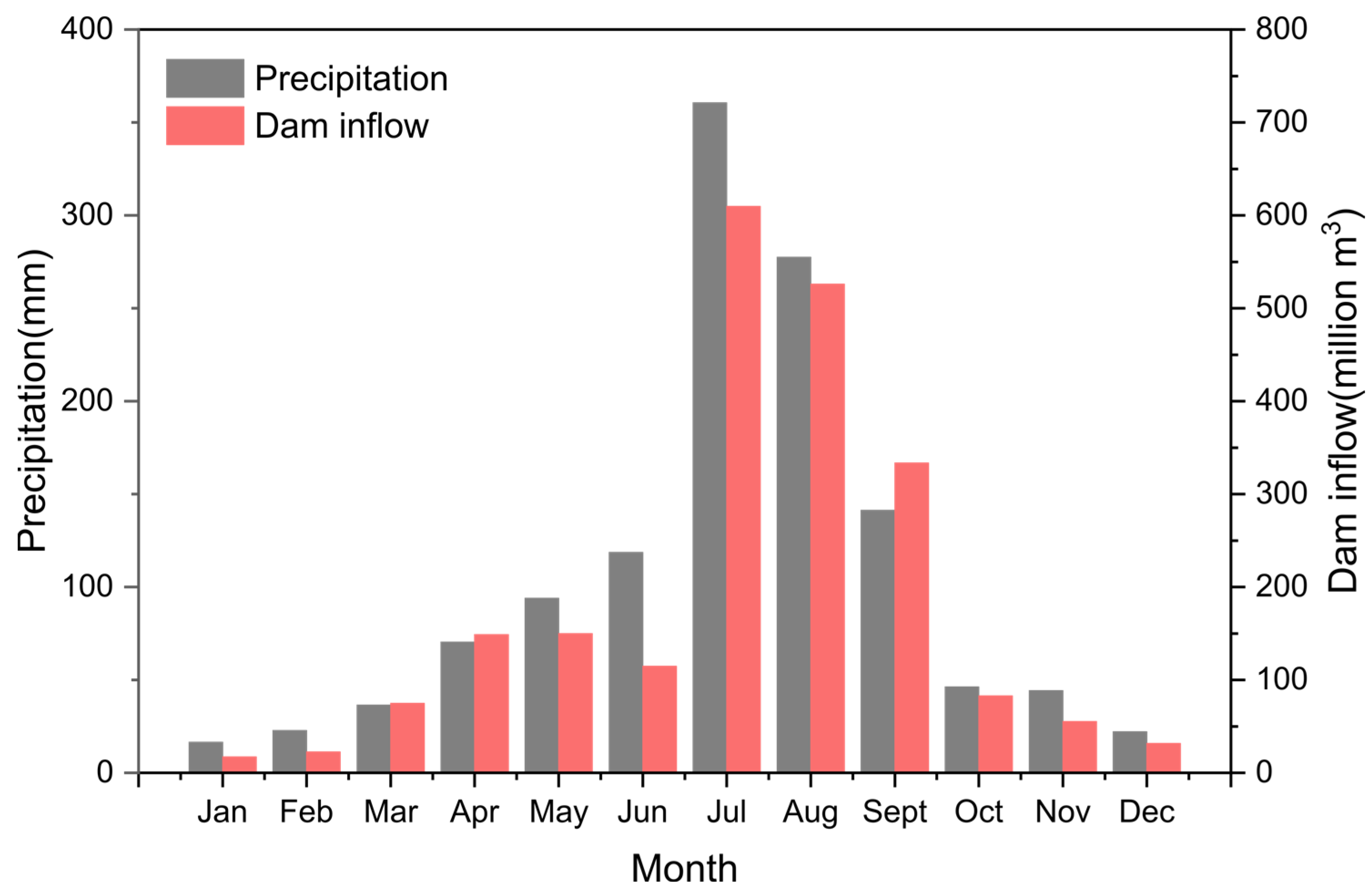
2.1. Description of the Study Area

The Soyang River Dam (SRD) in South Korea, located between 37°40′ to 38°30′ N and 127°40′ to 128°40′ E, is a crucial structure that plays a key role in controlling floods and droughts in the downstream area (Figure 1). The SRD has a 70 km2 reservoir area and supplies an average of 1.213 million m3 of water annually for residential, industrial, and irrigation use in the capital area. The 2703 km2 basin has an elevation range of 80–1693 m and is primarily composed of forest (89.5%), with smaller portions of agricultural land (5.7%), water (2.4%), and other lands (2.4%) [30]. The SRD is challenged by the large monthly variations in mean annual precipitation and dam inflow due to the Asian monsoon climate, making it difficult to manage water resources in downstream areas and establish an effective operational strategy (Figure 2). This situation is further complicated by the potential for frequent floods and droughts caused by seasonal fluctuations in precipitation due to climate change [34].

2.2. Data Collection

The flow into a dam can be influenced by various factors, including precipitation, temperature, evapotranspiration, land use, and anthropogenic activities [35]. However, it can be challenging to establish a relationship between these factors and the dam inflow. In addition, using all of these factors as input data for ML models can lead to difficulties in data preprocessing and collection. Mao et al. [36] found that dam inflow (i.e., streamflow) depends more strongly on variation in precipitation than temperature and evapotranspiration. In addition, Hong et al. [30] took into account the effect of prior weather conditions when predicting daily dam inflow using ML models by using weather and inflow data from the past one and two days. In this study, precipitation (Chuncheon and Injae stations) and SRD inflow data for 40 years (1980–2019) were obtained from the Korea Meteorological Administration (https://data.kma.go.kr, accessed on 31 March 2023) and Water Resources Management Information System (https://www.wamis.go.kr, accessed on 31 March 2023), respectively. The precipitation on the current day (Pt) and the precipitation (Pt−1 and Pt−2) and inflow data (It−1 and It−2) one and two days earlier were used as input for AS models to predict dam inflow (It). The heat map in Figure 3 shows the correlation for each input factor. The precipitation one day earlier (Pt−1) is most strongly correlated with the inflow on the day, followed by It−1, Pt−1, Pt−2, and It−2. Based on these input factors, the models were trained and validated using 35 years of data (1980–2015), and their predictive ability was tested using three years of data (2016–2019). Table 1 shows the details of the dataset used in the study.

2.3. Auto-Sklearn

AS is an AutoML framework based on the scikit-learn library that automates the process of finding the optimal ML pipeline for solving classification and regression problems within a limited time frame. The framework includes a total of 15 models, 14 feature preprocessing methods, and 4 data preprocessing methods.
To create an ensemble model, AS utilizes three techniques: meta-learning, Bayesian optimization, and ensemble selection. The meta-learning process in AS uses information from 140 pretrained reference datasets from OpenML to determine the best combination of models and hyperparameters for a given dataset [28]. During this process, the algorithm generates initial good hyperparameter configurations based on previous runs. By starting from these promising configurations, which have shown good performance on similar datasets, the efficiency of hyperparameter optimization can be significantly improved, resulting in a more accurate model [37].
After the meta-learning process, Bayesian optimization is applied to further refine the hyperparameters of top-performing models identified during meta-learning. This optimization algorithm, which uses Bayesian theory and a Gaussian process, is more efficient in finding the optimal hyperparameters by reducing the number of unnecessary configurations [38]. Finally, AS employs an ensemble selection technique [39] to create the final ensemble model, which is a combination of the top-performing models with varying weights, as determined by comparing their accuracy. The workflow of AS is illustrated in Figure 4.

2.4. MPE Model Development Using Split Datasets

Figure 5 illustrates the development of the MPE model using a combined approach with an AS. The combined approach trains two ensemble models using datasets separated by high and low inflow conditions, and the dam inflow is predicted by integrating the results. In contrast, the conventional approach trains an ensemble model using the whole training dataset and evaluates its performance on the test set.
In this study, to build the MPE model, the whole training dataset was divided into high and low inflow datasets using a high-inflow reference value of 100 m3/s, as suggested by Hong et al. [30]. Then, input factors highly correlated with inflow (i.e., precipitation on the day (Pt), precipitation from one day earlier (Pt−1), and inflow from one day earlier (It−1) were selected to determine the high-inflow reference value for the test set. The average and median values of these three factors for high-inflow (≥100 m3/s) in the whole training dataset were used to determine the high-inflow reference values. The reference values for Pt and Pt−1 were found to be 15.3 and 18.2 mm, respectively, based on the average value. The reference value for It−1, which showed a large deviation, was determined to be 197.4 m3/s using the median value.
These values are used to determine whether the MPE model will use an ensemble model for unique prediction or an ensemble model for low-flow prediction when given new input data for predicting dam inflow in the MPE model. In other words, the MPE model predicts the dam inflow by using the high-inflow prediction model if any of the three reference values (Pt, Pt−1, and It−1) are met in the test set; otherwise, the low-inflow prediction model is used. In both the conventional and combined approaches, the time_left_for_this_task and per_run_time_limit parameters of AS were set to 1 h and 360 s, respectively. The AS-based ensemble models developed through these two approaches were validated using 10-fold cross-validation, and their predictive performance was compared on the test set.

2.5. Performance Evaluation Metrics

In this study, we used the coefficient of determination (R2), Nash–Sutcliffe efficiency (NSE), root mean square errors (RMSE), and mean absolute error (MAE) to evaluate the predictive performance of the ensemble models developed through both the conventional and combined approaches. These statistical metrics are widely accepted for evaluating the accuracy of hydrological models [40]. The expressions were as follows:
R 2 = i = 1 n ( X i X ) ( Y i Y ) 2 i = 1 n ( X i X ) 2 i = 1 n ( Y i Y ) 2
N S E = 1 i = 1 n ( X i Y i ) 2 i = 1 n ( X i X ) 2
R M S E = i = 1 n ( X i Y i ) 2 n
M A E = i = 1 n X i Y i n
where  n  is the number of data samples in the time series.  X i  and  Y i  are the  i th observed and predicted dam inflow values, and  X  and  Y  are the averages of  X i  and  Y i , respectively.
R2 measures the strength of the linear relationship between observed and predicted values. It ranges from 0 to 1, a value of 1 indicates a perfect positive correlation. NSE is a normalized metric that measures the relative magnitude of the residual variance compared to the variance of the observations [41]. NSE values range from −∞ to 1, with a value of 1 being optimal. The RMSE and MAE are commonly used to measure the prediction errors of regression ML models. These metrics can be used together to determine the variation of the errors in a set of model predictions. The RMSE is always larger than or equal to the MAE, and the greater the difference between them, the greater the variance in individual errors in the sample [42]. The values of both metrics range from 0 to ∞, with values closer to 0 indicating better predictive performance.

3. Results and Discussion

3.1. Ensemble Modeling with Conventional and Combined Approaches for Inflow Prediction

Table 2 presents the results of the ensemble models constructed with conventional and combined approaches in AS. In Table 2, the weight indicates the importance of each model in the ensemble. The conventional approach comprised three models: multilayer perceptron (MLP), automatic relevance determination (ARD) regression, and gradient boosting (GB). The results showed that even when the same type of models are included in the ensemble configuration, their weights can be assigned differently based on data and feature preprocessing methods, as well as hyperparameters.
The ensemble model for high-inflow prediction consisted of extremely randomized trees (extra-trees), MLP, support vector regression (SVR), and ARD regression models. The extra-trees and MLP models had a significant impact, with weights of 0.46 and 0.40, respectively, demonstrating the models’ effectiveness in the training data and their significant contribution to accurate predictions. As a tree-based ensemble model, extra-trees builds multiple decision trees on randomly sampled subsets of data, displaying a high proficiency for capturing complex relationships. It is recognized for its reduction in variance and bias, as well as its computational efficiency and ability to handle noisy and nonlinear data [43]. The MLP can solve complex nonlinear relationships and is commonly used for high-dimensional problems. As demonstrated by Hong et al. [30], the MLP predicts high inflow more accurately than other models, such as the random forest and GB models. These results indicate that the high-inflow prediction ensemble model can effectively handle the complex and high-dimensional data structure, resulting in accurate predictions. In contrast, the low-inflow prediction ensemble model consisted of five models, with the SVR having the highest weight of 0.76. This highlights the effectiveness of SVR in accurately predicting low inflow compared to other models. The SVR has been widely and successfully applied in several studies for river flow prediction [44,45,46]. Furthermore, research conducted by Adamowski [47] and Yuan and Forshay [48] found that the SVR effectively captures nonlinear features of low flow, such as baseflow and groundwater. Sahoo et al. [49] also demonstrated the satisfactory performance of SVR in predicting monthly low flow for the Mahanadi river basin.
The study results confirmed the effectiveness of using separate training datasets for high inflow and low inflow in achieving a suitable ensemble configuration that reflects the unique characteristics of each dataset. In this study, the time_left_for_this_task and per_run_time_limit parameters, which determine the time budget in meta-learning for developing high-inflow and low-inflow prediction ensemble models, were set to the same value. The time budget in AS refers to the maximum time allowed for fitting and evaluating ML models for a specific dataset and may vary based on the dataset’s characteristics [50]. The time budget parameters can be adjusted by the user according to the size and complexity of the dataset, and available computational resources. Determining an optimal time budget that considers the characteristics of different datasets will be necessary for generating accurate and efficient ensemble results in the future. Furthermore, understanding the contribution of each model to the final prediction can be difficult, which may limit the interpretability of the AS-based ensemble model. Therefore, future research should evaluate the applicability of various analysis techniques such as SHAP (SHapley Additive exPlanations) [51] and LIME (Local Interpretable Model-Agnostic Explanations) [52] to increase the interpretability of the ensemble model.

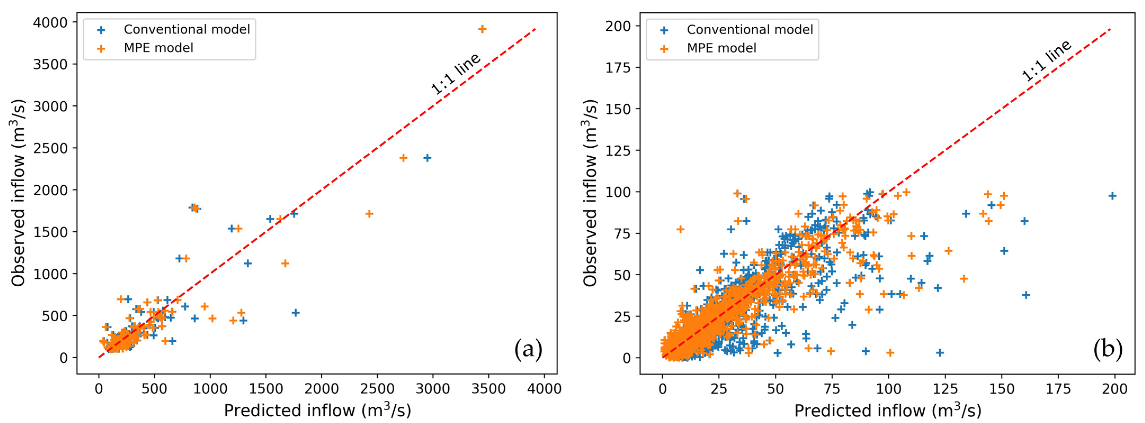
3.2. Comparison of Dam Inflow Prediction Performance

Figure 6 compares the time series of the predicted dam inflow with the observed values for the conventional and MPE models during the training and testing periods. Both models showed a reasonable prediction performance similar to previous studies [30,31,33] on dam inflow prediction using ML and deep learning (Table 3). However, the conventional model had limitations in predicting low inflow below 10 m3/s compared to the MPE model. This suggests that conventional AS-based ensemble models trained on the entire dataset may have been underfitted, resulting in an inaccurate capture of the characteristics of low-inflow data.
Figure 7b shows that the MPE model outperforms the conventional model for low-inflow values (<100 m3/s), while there is no significant difference between the models for high-inflow data (Figure 7a). Table 4 summarizes the performance of the two AS-based ensemble models for each test dataset. The MPE model improves RMSE and MAE by 4.2% and 1.6%, respectively, and increases R2 and NSE by 2.5% and 35.8%, respectively, for low-inflow data. For high-inflow data, it reduces RMSE and MAE by 22.1% and 24.9%, respectively, and increases R2 and NSE by 21.9% and 35.8%, respectively.
This improved performance can be attributed to the MPE model’s combined approach, where models are trained separately for high-inflow and low-inflow datasets, allowing for the optimization of the models using the Bayesian optimization algorithm in AS. In contrast, conventional model approaches trained on the entire dataset are less likely to be optimized for each flow regime, leading to poor predictive ability and low-flow regimes. This highlights the importance of optimizing models for different flow regimes, especially low-flow regimes, to improve their predictive ability.
It is noteworthy that the prediction performance of the AS-based ensemble models for dam inflow does not show a significant difference compared to other standalone and combined ML models. The performance of an ML model for a specific dataset can also be improved by the efforts of experts, rather than relying on meta-learning-based AS [53]. This means that AS cannot guarantee the development of the optimal prediction model for a given dataset. Furthermore, Tanaka et al. [54] found that the accuracy of an AS-based ensemble model in predicting the number of defects in software modules was comparable to that of an RF model. Shi et al. [53] also showed that the AS-based ensemble model had high performance in predicting concrete compressive strength, but there was no significant difference between its performance and that of an independent model built by an expert. However, their studies commonly demonstrated that even without extensive knowledge of ML, AS can still be utilized to construct a robust ensemble model with satisfactory predictive performance.
The development of a robust ensemble model is time- and labor-intensive and can be difficult for nonexperts. From these perspectives, AS is considered useful in efficiently developing robust ensemble models objectively and rationally, minimizing user subjectivity, and without manual processes such as preprocessing, hyperparameter optimization, and model combination. The ensemble model, based on the combined approach in this study is expected to improve the model prediction’s accuracy by resolving the imbalance of the given dataset.

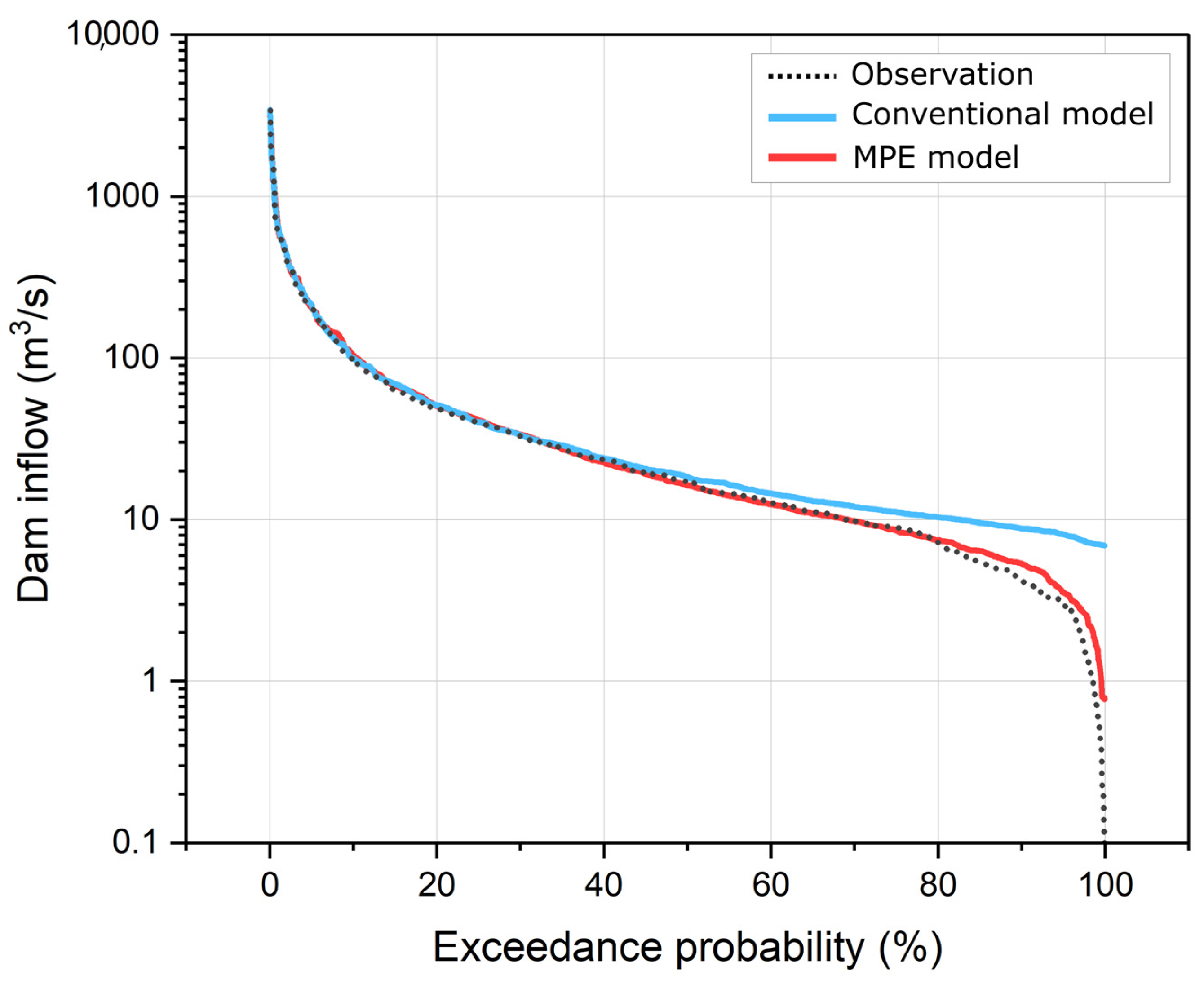
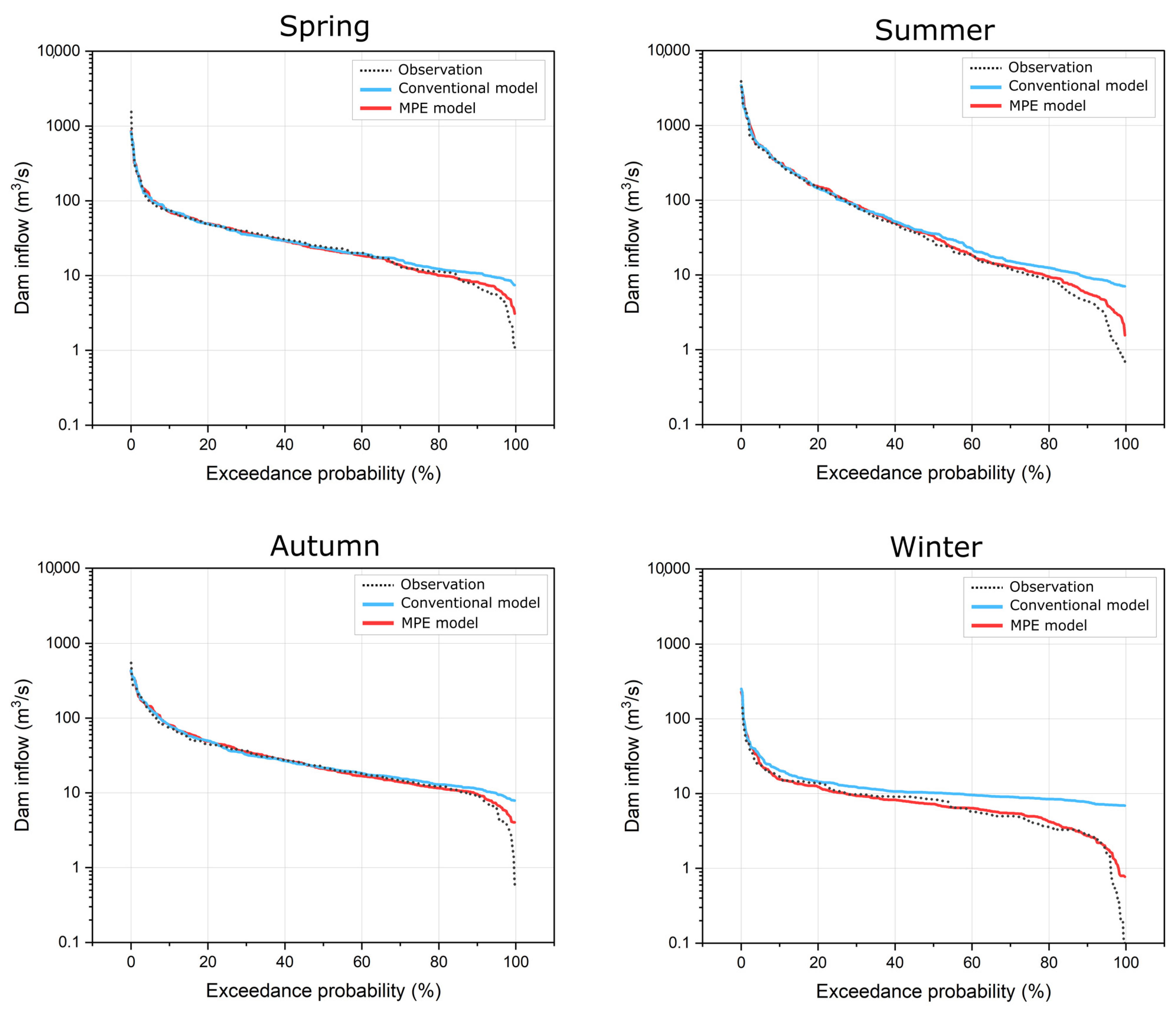
3.3. Comparison of AS-Based Ensemble Models for Dam Inflow Prediction Using FDC Analysis

The flow duration curve (FDC) is a cumulative frequency plot that displays the percentage of time-specified discharges that were equaled or exceeded during a given period [55]. The FDC is generally divided into five zones, representing different hydrologic conditions of a stream: high flow (0–10%), moist conditions (10–40%), mid-range flow (40–60%), dry conditions (60–90%), and low flow (90–100%). This can help identify sustainable water resource management plans. In this study, AS-based ensemble models were developed using conventional and combined approaches to predict dam inflow, and their performance was evaluated using FDC.
Figure 8 shows the FDCs for the dam inflow test dataset predicted by the MPE and conventional models. The AS-based ensemble models had good agreement with the observed values (<40% exceedance probability), while the conventional model performed poorly towards the lower portion of FDCs. As shown in Table 5, the MPE model performed better for the intervals below the mid-range flow range and yielded low-inflow data more accurately than the conventional model for all seasons (Figure 9). These results suggest that, although both ensemble models predicted the high inflow in the flood period with satisfactory performance, the combined approach is needed to capture the low-inflow behavior in the nonflood period well.
More specifically, Figure 10 compares the observed and predicted low inflow values using the models for each season (>60% exceedance probability), showing that the MPE model had higher R2 and NSE than the conventional model, reducing RMSE and MAE by 58.8–88.5% and 54.1–89.9%, respectively (Table 6). This indicates that the integration of ensemble models for high and low flows is necessary to produce accurate dam inflow prediction data that takes into account the seasonal characteristics of floods and dry periods. Through the above results, we confirm that the MPE model is suitable for generating seasonal low-inflow data for decision-making in dam operation, especially in the SRD basin, where 61% (756.7 mm) of rainfall occurs from June to August due to the Asian monsoon. The water level of a dam can be affected by various factors, including evapotranspiration, topography, and groundwater; however, it is directly affected by the inflow from the watershed upstream of the dam [56]. Climate change may cause changes in streamflow regimes, leading to flow variability and extreme seasonality [57,58]. Hence, the MPE model can provide accurate and consistent dam inflow prediction results for both flood and nonflood seasons, allowing for appropriate hydrological manipulations to ensure water storage and prepare for potential flood damage in downstream regions.

4. Conclusions

In this study, we aimed to develop a robust and efficient AS-based ensemble model for predicting multi-inflow in dam reservoirs. Our approach involved the development of the MPE model, which combined two types of datasets for high and low inflow conditions to predict multi-inflow. Our results show that the MPE model outperforms a conventional model in predicting both high and low inflow conditions, demonstrating the effectiveness of our ensemble approach in addressing the imbalance between high and low inflow observations in the dataset. Additionally, the MPE model was found to capture the characteristics of each flow regime and make more accurate predictions for each condition.
Our study contributes to the field of water resource management by providing a reliable method for predicting dam inflow that can inform better decision-making and planning for flood and nonflood periods. Our findings highlight the importance of using an ensemble approach to overcome the challenges associated with predicting multi-inflow and suggest that the AS-based ensemble model can be used as a tool by nonexperts without domain knowledge related to ML.
Although our study presents promising results, it is not without limitations. For instance, the study only used data from a single dam reservoir and may not generalize to other regions with different hydrological conditions. Furthermore, although we demonstrated the effectiveness of our ensemble approach, more research is needed to evaluate the robustness of the model in the face of uncertainty and other potential factors that may affect its predictive performance.
Future research could explore the potential impact of model uncertainty analysis on the predictive performance of the MPE model and its ability to make reliable predictions for various inflow conditions. Additionally, improving the library for AS to generate integrated prediction results using various ensemble models trained according to data standards set by the user could eliminate the need for manual separation of datasets and enable nonexperts to use AS-based ensemble model development.
Overall, our study underscores the scientific value added to the field of water resource management by providing a reliable method for predicting dam inflow using an ensemble approach. Our results have important implications for policymakers and decision-makers, highlighting the need to invest in the development of robust and efficient AS-based ensemble models for predicting multi-inflow in dam reservoirs.

Author Contributions

Conceptualization: K.J.L., J.K. and S.L.; Methodology: S.L., G.L. and J.H.B.; Formal analysis and investigation: D.Y.; Writing—original draft preparation: S.L. Writing—review and editing: J.K. and J.H.; Supervision: K.J.L. All authors have read and agreed to the published version of the manuscript.

Funding

This work has been supported by the Korea Environment Industry & Technology Institute (KEITI) through the Aquatic Ecosystem Conservation Research Program funded by the Korean Ministry of Environment (MOE), grant number 2020003030004.

Data Availability Statement

Some of the data, models, or codes that support the findings of this study are available from the corresponding author on reasonable request.

Conflicts of Interest

The authors declare that they have no known competing financial interests or personal relationships that could have appeared to influence the work reported in this paper.

References

  1. Simonovic, S.P. Bringing Future Climatic Change into Water Resources Management Practice Today. Water Resour. Manag. 2017, 31, 2933–2950. [Google Scholar] [CrossRef]
  2. Zhao, L.; Xia, J.; Sobkowiak, L.; Wang, Z.; Guo, F. Spatial Pattern Characterization and Multivariate Hydrological Frequency Analysis of Extreme Precipitation in the Pearl River Basin, China. Water Resour. Manag. 2012, 26, 3619–3637. [Google Scholar] [CrossRef]
  3. Samuels, R.; Rimmer, A.; Alpert, P. Effect of Extreme Rainfall Events on the Water Resources of the Jordan River. J. Hydrol. 2009, 375, 513–523. [Google Scholar] [CrossRef]
  4. Ehsani, N.; Vörösmarty, C.J.; Fekete, B.M.; Stakhiv, E.Z. Reservoir Operations under Climate Change: Storage Capacity Options to Mitigate Risk. J. Hydrol. 2017, 555, 435–446. [Google Scholar] [CrossRef]
  5. Prasanchum, H.; Kangrang, A. Optimal Reservoir Rule Curves under Climatic and Land Use Changes for Lampao Dam Using Genetic Algorithm. KSCE J. Civ. Eng. 2018, 22, 351–364. [Google Scholar] [CrossRef]
  6. Naz, B.S.; Kao, S.-C.; Ashfaq, M.; Gao, H.; Rastogi, D.; Gangrade, S. Effects of Climate Change on Streamflow Extremes and Implications for Reservoir Inflow in the United States. J. Hydrol. 2018, 556, 359–370. [Google Scholar] [CrossRef]
  7. Momiyama, S.; Sagehashi, M.; Akiba, M. Assessment of the Climate Change Risks for Inflow into Sagami Dam Reservoir Using a Hydrological Model. J. Water Clim. Chang. 2020, 11, 367–379. [Google Scholar] [CrossRef]
  8. Xu, S.; Chen, Y.; Xing, L.; Li, C. Baipenzhu Reservoir Inflow Flood Forecasting Based on a Distributed Hydrological Model. Water 2021, 13, 272. [Google Scholar] [CrossRef]
  9. Alizadeh, F.; Gharamaleki, A.F.; Jalilzadeh, M.; Akhoundzadeh, A. Prediction of River Stage-Discharge Process Based on a Conceptual Model Using EEMD-WT-LSSVM Approach. Water Resour. 2020, 47, 41–53. [Google Scholar] [CrossRef]
  10. Shelke, M.; Londhe, S.; Dixit, P.R.; Kolhe, P. Simulation of reservoir inflow using HEC-HMS; 2022. In Proceedings of the HYDRO 2021-International Conference (Hydraulics, Water Resources and Coastal Engineering), Pune, India, 23–25 December 2021. [Google Scholar]
  11. Wibowo, H.; Ridwansyah, I.; Rahmat, A. Evaluating inflow result from SWAT model at Singkarak Lake under limited data. In IOP Conference Series: Earth and Environmental Science, Proceedings of the 5th Indonesian Society of Limnology (MLI) Congress and International Conference, Online, 2–3 December 2021; IOP Publishing Ltd.: Bristol, UK, 2022; Volume 1062. [Google Scholar] [CrossRef]
  12. Zhang, X.; Wang, H.; Peng, A.; Wang, W.; Li, B.; Huang, X. Quantifying the Uncertainties in Data-Driven Models for Reservoir Inflow Prediction. Water Resour. Manag. 2020, 34, 1479–1493. [Google Scholar] [CrossRef]
  13. Tran, T.D.; Tran, V.N.; Kim, J. Improving the Accuracy of Dam Inflow Predictions Using a Long Short-Term Memory Network Coupled with Wavelet Transform and Predictor Selection. Mathematics 2021, 9, 551. [Google Scholar] [CrossRef]
  14. Ahmad, S.K.; Hossain, F. A Generic Data-Driven Technique for Forecasting of Reservoir Inflow: Application for Hydropower Maximization. Environ. Model. Softw. 2019, 119, 147–165. [Google Scholar] [CrossRef]
  15. Apaydin, H.; Feizi, H.; Sattari, M.T.; Colak, M.S.; Shamshirband, S.; Chau, K.-W. Comparative Analysis of Recurrent Neural Network Architectures for Reservoir Inflow Forecasting. Water 2020, 12, 1500. [Google Scholar] [CrossRef]
  16. Herbert, Z.C.; Asghar, Z.; Oroza, C.A. Long-Term Reservoir Inflow Forecasts: Enhanced Water Supply and Inflow Volume Accuracy Using Deep Learning. J. Hydrol. 2021, 601, 126676. [Google Scholar] [CrossRef]
  17. Mosavi, A.; Ozturk, P.; Chau, K.W. Flood Prediction Using Machine Learning Models: Literature Review. Water 2018, 10, 1536. [Google Scholar] [CrossRef] [Green Version]
  18. Zuo, G.; Luo, J.; Wang, N.; Lian, Y.; He, X. Decomposition Ensemble Model Based on Variational Mode Decomposition and Long Short-Term Memory for Streamflow Forecasting. J. Hydrol. 2020, 585, 124776. [Google Scholar] [CrossRef]
  19. Yang, S.; Yang, D.; Chen, J.; Santisirisomboon, J.; Lu, W.; Zhao, B. A Physical Process and Machine Learning Combined Hydrological Model for Daily Streamflow Simulations of Large Watersheds with Limited Observation Data. J. Hydrol. 2020, 590, 125206. [Google Scholar] [CrossRef]
  20. Tyralis, H.; Papacharalampous, G.; Langousis, A. Super Ensemble Learning for Daily Streamflow Forecasting: Large-Scale Demonstration and Comparison with Multiple Machine Learning Algorithms. Neural Comput. Appl. 2021, 33, 3053–3068. [Google Scholar] [CrossRef]
  21. Rajesh, M.; Anishka, S.; Viksit, P.S.; Arohi, S.; Rehana, S. Improving Short-Range Reservoir Inflow Forecasts with Machine Learning Model Combination. Water Resour. Manag. 2023, 37, 75–90. [Google Scholar] [CrossRef]
  22. Paul, T.; Raghavendra, S.; Ueno, K.; Ni, F.; Shin, H.; Nishino, K.; Shingaki, R. Forecasting of reservoir inflow by the combination of deep learning and conventional machine learning. In Proceedings of the 2021 International Conference on Data Mining Workshops (ICDMW), Auckland, New Zealand, 7–10 December 2021; pp. 558–565. [Google Scholar]
  23. Rezaie-Balf, M.; Naganna, S.R.; Kisi, O.; El-Shafie, A. Enhancing Streamflow Forecasting Using the Augmenting Ensemble Procedure Coupled Machine Learning Models: Case Study of Aswan High Dam. Hydrol. Sci. J. 2019, 64, 1629–1646. [Google Scholar] [CrossRef]
  24. Truong, A.; Walters, A.; Goodsitt, J.; Hines, K.; Bruss, C.B.; Farivar, R. Towards automated machine learning: Evaluation and comparison of automl approaches and tools. In Proceedings of the 2019 IEEE 31st International Conference on Tools with Artificial Intelligence (ICTAI), Portland, OR, USA, 4–6 November 2019; pp. 1471–1479. [Google Scholar]
  25. Shi, X.; Wong, Y.D.; Chai, C.; Li, M.Z.-F. An Automated Machine Learning (AutoML) Method of Risk Prediction for Decision-Making of Autonomous Vehicles. IEEE Trans. Intell. Transp. Syst. 2020, 22, 7145–7154. [Google Scholar] [CrossRef]
  26. Tsiakmaki, M.; Kostopoulos, G.; Kotsiantis, S.; Ragos, O. Implementing AutoML in Educational Data Mining for Prediction Tasks. Appl. Sci. 2020, 10, 90. [Google Scholar] [CrossRef] [Green Version]
  27. Babaeian, E.; Paheding, S.; Siddique, N.; Devabhaktuni, V.K.; Tuller, M. Estimation of Root Zone Soil Moisture from Ground and Remotely Sensed Soil Information with Multisensor Data Fusion and Automated Machine Learning. Remote Sens. Environ. 2021, 260, 112434. [Google Scholar] [CrossRef]
  28. Feurer, M.; Klein, A.; Eggensperger, K.; Springenberg, J.T.; Blum, M.; Hutter, F. Efficient and robust automated machine learning. In Advances in Neural Information Processing Systems 28 (NIPS 2015); Neural Information Processing Systems Foundation, Inc. (NeurIPS): La Jolla, CA, USA, 2015; pp. 2962–2970. [Google Scholar]
  29. Han, H.; Kim, D.; Wang, W.; Kim, H.S. Dam Inflow Prediction Using Large-Scale Climate Variability and Deep Learning Approach: A Case Study in South Korea. Water Supply 2023, 23, 934–947. [Google Scholar] [CrossRef]
  30. Hong, J.; Lee, S.; Bae, J.H.; Lee, J.; Park, W.J.; Lee, D.; Kim, J.; Lim, K.J. Development and Evaluation of the Combined Machine Learning Models for the Prediction of Dam Inflow. Water 2020, 12, 2927. [Google Scholar] [CrossRef]
  31. Moon, G.-H.; Kim, S.-H.; Bae, D.-H. Development and Evaluation of ANFIS-Based Conditional Dam Inflow Prediction Method Using Flow Regime. J. Korea Water Resour. Assoc. 2018, 51, 607–616. [Google Scholar] [CrossRef]
  32. Zhang, W.; Wang, H.; Lin, Y.; Jin, J.; Liu, W.; An, X. Reservoir Inflow Predicting Model Based on Machine Learning Algorithm via Multi-Model Fusion: A Case Study of Jinshuitan River Basin. IET Cyber-Syst. Robot. 2021, 3, 265–277. [Google Scholar] [CrossRef]
  33. Choi, H.S.; Kim, J.H.; Lee, E.H.; Yoon, S.-K. Development of a Revised Multi-Layer Perceptron Model for Dam Inflow Prediction. Water 2022, 14, 1878. [Google Scholar] [CrossRef]
  34. Lee, M.H.; Im, E.S.; Bae, D.H. Future Projection in Inflow of Major Multi-Purpose Dams in South Korea. J. Wetl. Res. 2019, 21, 107–116. [Google Scholar]
  35. Xu, S.; Qin, M.; Ding, S.; Zhao, Q.; Liu, H.; Li, C.; Yang, X.; Li, Y.; Yang, J.; Ji, X. The Impacts of Climate Variation and Land Use Changes on Streamflow in the Yihe River, China. Water 2019, 11, 887. [Google Scholar] [CrossRef] [Green Version]
  36. Mao, T.; Wang, G.; Zhang, T. Impacts of Climatic Change on Hydrological Regime in the Three-River Headwaters Region, China, 1960–2009. Water Resour. Manag. 2016, 30, 115–131. [Google Scholar] [CrossRef]
  37. Feurer, M.; Springenberg, J.; Hutter, F. Initializing Bayesian Hyperparameter Optimization via Meta-Learning. In Proceedings of the Twenty-Ninth AAAI Conference on Artificial Intelligence, Austin, TX USA, 25–30 January 2015; Volume 29. [Google Scholar] [CrossRef]
  38. Pelikan, M.; Goldberg, D.E.; Cantú-Paz, E. BOA: The bayesian optimization algorithm. In Proceedings of the Genetic and Evolutionary Computation Conference GECCO-99, Orlando, FL, USA, 13–17 July 1999; Volume 1, pp. 525–532. [Google Scholar]
  39. Caruana, R.; Niculescu-Mizil, A.; Crew, G.; Ksikes, A. Ensemble Selection from Libraries of Models. In Proceedings of the twenty-first international conference on Machine learning, Banff, AB, Canada, 4–8 July 2004. [Google Scholar]
  40. Moriasi, D.; Gitau, M.; Pai, N.; Daggupati, P. Hydrologic and Water Quality Models: Performance Measures and Evaluation Criteria. Trans. ASABE Am. Soc. Agric. Biol. Eng. 2015, 58, 1763–1785. [Google Scholar] [CrossRef] [Green Version]
  41. Nash, J.E.; Sutcliffe, J.V. River Flow Forecasting through Conceptual Models Part I—A Discussion of Principles. J. Hydrol. 1970, 10, 282–290. [Google Scholar] [CrossRef]
  42. Motaghian, H.R.; Mohammadi, J. Spatial Estimation of Saturated Hydraulic Conductivity from Terrain Attributes Using Regression, Kriging, and Artificial Neural Networks. Pedosphere 2011, 21, 170–177. [Google Scholar] [CrossRef]
  43. Galelli, S.; Castelletti, A. Assessing the Predictive Capability of Randomized Tree-Based Ensembles in Streamflow Modelling. Hydrol. Earth Syst. Sci. 2013, 17, 2669–2684. [Google Scholar] [CrossRef] [Green Version]
  44. Adnan, R.; Yuan, X.; Kisi, O.; Yuan, Y. Streamflow Forecasting Using Artificial Neural Network and Support Vector Machine Models. Am. Sci. Res. J. Eng. Technol. Sci. 2017, 29, 286–294. [Google Scholar]
  45. Yaghoubi, B.; Hosseini, S.A.; Nazif, S. Monthly Prediction of Streamflow Using Data-Driven Models. J. Earth Syst. Sci. 2019, 128, 141. [Google Scholar] [CrossRef] [Green Version]
  46. Yaseen, Z.M.; El-shafie, A.; Jaafar, O.; Afan, H.A.; Sayl, K.N. Artificial Intelligence Based Models for Stream-Flow Forecasting: 2000–2015. J. Hydrol. 2015, 530, 829–844. [Google Scholar] [CrossRef]
  47. Adamowski, J. Using Support Vector Regression to Predict Direct Runoff, Base Flow and Total Flow in a Mountainous Watershed with Limited Data in Uttaranchal, India. Ann. Warsaw Univ. Life Sci. SGGW. L. Reclam. 2013, 45, 71–83. [Google Scholar] [CrossRef]
  48. Yuan, L.; Forshay, K.J. Enhanced Streamflow Prediction with SWAT Using Support Vector Regression for Spatial Calibration: A Case Study in the Illinois River Watershed, U.S. PLoS ONE 2021, 16, e0248489. [Google Scholar] [CrossRef]
  49. Sahoo, B.B.; Jha, R.; Singh, A.; Kumar, D. Application of Support Vector Regression for Modeling Low Flow Time Series. KSCE J. Civ. Eng. 2019, 23, 923–934. [Google Scholar] [CrossRef]
  50. Eldeeb, H.; Matsuk, O.; Maher, M.; Eldallal, A.; Sakr, S. The Impact of Auto-Sklearn’s Learning Settings: Meta-Learning, Ensembling, Time Budget, and Search Space Size. In Proceedings of the EDBT/ICDT Workshops, Nicosia, Cyprus, 23–26 March 2021. [Google Scholar]
  51. Lundberg, S.; Erion, G.; Lee, S.-I. Consistent Individualized Feature Attribution for Tree Ensembles. ArXiv 2018. [Google Scholar] [CrossRef]
  52. Ribeiro, M.T.; Singh, S.; Guestrin, C. “Why should I trust you?”: Explaining the predictions of any classifier. In Proceedings of the 22nd ACM SIGKDD International Conference on Knowledge Discovery and Data Mining; Association for Computing Machinery: New York, NY, USA, 2016; pp. 1135–1144. [Google Scholar]
  53. Shi, M.; Shen, W. Automatic Modeling for Concrete Compressive Strength Prediction Using Auto-Sklearn. Buildings 2022, 12, 1406. [Google Scholar] [CrossRef]
  54. Tanaka, K.; Monden, A.; Yücel, Z. Prediction of Software Defects Using Automated Machine Learning. In Proceedings of the 2019 20th IEEE/ACIS International Conference on Software Engineering, Artificial Intelligence, Net-working and Parallel/Distributed Computing (SNPD), Toyama, Japan, 8–11 July 2019; pp. 490–494. [Google Scholar]
  55. Searcy, J.K. Flow-Duration Curves; US Government Printing Office: Washington, DC, USA, 1959. [Google Scholar]
  56. Yokoo, Y.; Sivapalan, M. Towards Reconstruction of the Flow Duration Curve: Development of a Conceptual Framework with a Physical Basis. Hydrol. Earth Syst. Sci. 2011, 15, 2805–2819. [Google Scholar] [CrossRef] [Green Version]
  57. Brunner, M.I.; Melsen, L.A.; Newman, A.J.; Wood, A.W.; Clark, M.P. Future Streamflow Regime Changes in the United States: Assessment Using Functional Classification. Hydrol. Earth Syst. Sci. 2020, 24, 3951–3966. [Google Scholar] [CrossRef]
  58. Chai, Y.; Li, Y.; Yang, Y.; Zhu, B.; Li, S.; Xu, C.; Liu, C. Influence of Climate Variability and Reservoir Operation on Streamflow in the Yangtze River. Sci. Rep. 2019, 9, 5060. [Google Scholar] [CrossRef] [Green Version]
Figure 1. Study area.
Hydrology 10 00090 g001
Figure 2. Average annual precipitation and dam inflow in the study area.
Hydrology 10 00090 g002
Figure 3. Heat map showing correlation for each input factor.
Hydrology 10 00090 g003
Figure 4. Workflow of AS.
Hydrology 10 00090 g004
Figure 5. Development of the MPE model.
Hydrology 10 00090 g005
Figure 6. Comparison of predicted and observed inflow using both models with training (a) and test (b) data.
Hydrology 10 00090 g006
Figure 7. Scatter plots of predictions of both models using separate test data for (a) ≥100 m3/s and (b) <100 m3/s.
Hydrology 10 00090 g007
Figure 8. FDCs of observed inflow and inflow predicted by both models during the whole test period.
Hydrology 10 00090 g008
Figure 9. FDCs of predicted and observed seasonal inflows.
Hydrology 10 00090 g009
Figure 10. Scatter plots of predictions of both models for seasonal low inflows.
Hydrology 10 00090 g010
Table 1. Dataset used to develop AS ensemble model.
ModelInput VariablesTarget VariablePeriod
Training and validation dataset (n =13,148)It−1, It−2
Pt, Pt−1, Pt−2
It1980–2015
Test dataset (n = 1461)It−1, It−2
Pt, Pt−1, Pt−2
It2016–2019
t: time (day) index.
Table 2. Ensemble results of AS using conventional and combined approaches.
ModelDatasetWeightData Preprocessing MethodFeature Preprocessing MethodHyperparametersModel Type
Conventional modelAll data0.20encoding = ‘one_hot_encoding’, imputation = ‘mean’, rescaling = ‘standardize’extra_trees_preproc_for_regressionactivation = ‘relu’, alpha = 6.03 × 10⁻⁷ early_stop = ‘valid’, hidden_layer_depth = 3, learning_rate_init = 0.0001, n_iter_no_change = 32, num_nodes_per_layer = 100, solver = ‘adam’MLP
0.04encoding = ‘one_hot_encoding’, imputation = ‘median’, rescaling = ‘minmax’polynomialactivation = ‘relu’, alpha = 6.11 × 10⁻⁵, early_stop = ‘valid’, hidden_layer_depth = 3, learning_rate_init = 0.0002, n_iter_no_change = 32, num_nodes_per_layer = 101, solver = ‘adam’MLP
0.38imputation = ‘mean’polynomialn_iter = 300, tol = 0.0091, alpha_1 = 4.70 × 10⁻⁵, alpha_2 = 0.0006, lambda_1 = 7.58 × 10⁻¹⁰, lambda_2= 3.92 × 10⁻⁸, threshold_lambda= 4052ARD regression
0.26encoding = ‘one_hot_encoding’, imputation = ‘median’, rescaling = ‘standardize’polynomialmax_depth = ‘none’, max_leaf_nodes = 28, min_samples_leaf = 6, n_iter_no_change = 5, learning_rate = 0.1329, l2_regularization = 8.22 × 10⁻¹⁰, early_stop = ‘valid’GB
0.04encoding = ‘one_hot_encoding’, imputation = ‘mean’polynomialmax_depth = ‘none’, max_leaf_nodes = 31, min_samples_leaf = 25, n_iter_no_change = 7, learning_rate = 0.1239, l2_regularization = 6.08 × 10⁻¹⁰, early_stop = ‘train’GB
0.08encoding = ‘one_hot_encoding’, imputation = ‘median’, rescaling = ‘minmax’polynomialmax_depth = ‘none’, max_leaf_nodes = 26, min_samples_leaf = 6, n_iter_no_change = 20, validation_fraction = 0.08, learning_rate = 0.1530, l2_regularization = 0.013, early_stop = ‘valid’GB
MPE modelHigh-inflow0.46imputation= ‘most_frequent’, rescaling = ‘minmax’polynomialmax_depth = ‘none’, max_features = 0.979, max_leaf_nodes = ‘none’, min_samples_leaf = 1, min_samples_split = 4Extra-trees
0.40encoding = ‘one_hot_encoding’, imputation = ‘mean’, rescaling = ‘standardize’extra_trees_preproc_for_regressionactivation = ‘relu’, alpha = 6.03 × 10⁻⁷, early_stop = ‘valid’, hidden_layer_depth = 3, learning_rate_init = 0.0001, n_iter_no_change = 32, num_nodes_per_layer = 100, solver = ‘adam’MLP
0.10encoding = ‘one_hot_encoding’, imputation = ‘mean’, rescaling = ‘minmax’fast_icakernel = ‘rbf’, degree = 3, gamma = 0.201, tol = 0.021, C = 194.03, epsilon = 0.001, max_iter = −1SVR
0.04encoding = ‘one_hot_encoding’, imputation = ‘most_frequent’, rescaling = ‘robust_scaler’select_rates_regressionn_iter = 300, tol = 0.0007, alpha_1 = 2.76 × 10⁻⁵, alpha_2= 9.50 × 10⁻⁷, lambda_1 = 6.51 × 10⁻⁹, lambda_2 = 4.24 × 10⁻⁷, threshold_lambda = 78,251.5, fit_intercept = ‘ture’ARD regression
Low-inflow0.76imputation = ‘most_frequent’, rescaling = ‘minmax’fast_icakernel = ‘rbf’, degree = 2, gamma = 0.032, tol = 0.0034, C = 7277.3, epsilon = 0.001, max_iter = −1SVR
0.06encoding = ‘one_hot_encoding’, imputation = ‘median’, rescaling = ‘minmax’polynomialactivation = ‘relu’, alpha = 6.11 × 10⁻⁵, early_stop = ‘valid’, hidden_layer_depth = 3, learning_rate_init = 0.0003, n_iter_no_change = 32, num_nodes_per_layer = 101, solver = ‘adam’MLP
0.06imputation = ‘mean’polynomialn_iter= 300, tol = 0.0091, alpha_1 = 4.70 × 10⁻⁵, alpha_2 = 0.0006, lambda_1 = 7.58 × 10⁻¹⁰, lambda_2 = 3.92 × 10⁻⁸, threshold_lambda = 4052, fit_intercept = ‘ture’ARD regression
0.04imputation = ‘mean’, rescaling = ‘power_transformer’euclideann_estimator = 140, learning_rate = 0.2841, loss = ‘exponential’, max_depth = 8Adaboost
0.08encoding = ‘one_hot_encoding’, imputation = ‘mean’, rescaling = ‘standardize’no_preprocessingmax_depth = ‘none’, max_leaf_nodes = 9, min_samples_leaf = 2, n_iter_no_change = 20, learning_rate = 0.0913, l2_regularization = 0.0057, early_stop = ‘train’GB
Table 3. Comparison of performance of both models on training and test data.
ModelTraining Period (1985–2015)Test Period (2016–2019)
R2NSERMSEMAER2NSERMSEMAE
Conventional model0.910.9070.7419.510.860.8567.1817.21
MPE model0.950.9455.4814.010.880.8763.9315.29
Table 4. Comparison of performance of both models on separate test data.
PeriodModelInflow
Condition
R2NSERMSEMAE
TrainingConventional model≥100 m3/s0.890.88190.2189.99
<100 m3/s0.620.4816.268.79
MPE model≥100 m3/s0.930.93149.7665.65
<100 m3/s0.790.7311.696.15
TestingConventional model≥100 m3/s0.800.80210.76103.13
<100 m3/s0.640.5313.917.92
MPE model≥100 m3/s0.820.82201.91101.50
<100 m3/s0.780.7210.845.95
Table 5. Comparison of performance of both models for flow regimes.
ModelMetricHigh FlowMoist
Conditions
Mid–Range FlowDry
Conditions
Low Flow
Conventional modelR20.970.990.990.970.97
NSE0.970.970.76−0.43−19.90
RMSE78.672.931.502.935.40
MAE28.082.141.412.775.37
MPE modelR20.961.000.990.980.97
NSE0.960.970.950.950.41
RMSE90.963.040.680.520.91
MAE34.532.130.560.420.88
Table 6. Comparison of performance of both models for seasonal low inflows.
ModelMetricSpring (Mar–May)Summer (Jun–Aug)Autumn (Sep–Nov)Winter (Dec–Feb)
Conventional modelR20.950.970.970.93
NSE0.650.030.68−9.20
RMSE2.764.542.384.80
MAE2.244.431.814.74
MPE modelR20.970.990.990.96
NSE0.950.930.950.86
RMSE1.021.260.980.55
MAE0.851.160.830.48
Disclaimer/Publisher’s Note: The statements, opinions and data contained in all publications are solely those of the individual author(s) and contributor(s) and not of MDPI and/or the editor(s). MDPI and/or the editor(s) disclaim responsibility for any injury to people or property resulting from any ideas, methods, instructions or products referred to in the content.

