
Evaluating Methods of Streamflow Timing to Approximate Snowmelt Contribution in High-Elevation Mountain Watersheds


Abstract
:1. Introduction
2. Materials and Methods
3. Results
4. Discussion
4.1. Method Evaluation
4.2. Trends in Streamflow Timing Metrics
5. Conclusions
Author Contributions
Funding
Data Availability Statement
Conflicts of Interest
Appendix A. Overview of Watersheds Analyzed


| Watershed Name | HUC | Latitude (°N) | Longitude (°W) | Elevation (m) | Area (km2) |
|---|---|---|---|---|---|
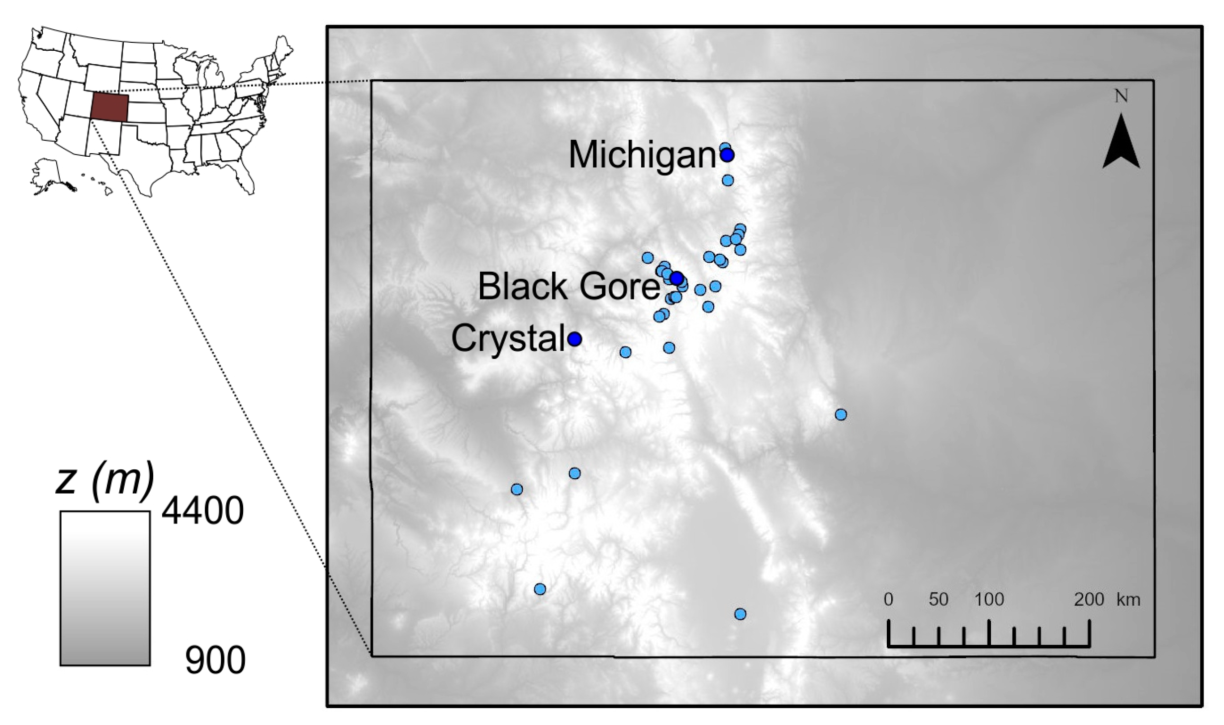
| Bighorn Creek | 09066100 | 39.63999 | −106.293 | 2629 | 12 |
| Black Gore Creek * | 09066000 | 39.59637 | −106.265 | 2789 | 32 |
| Blue River | 09046600 | 39.45582 | −106.032 | 2749 | 319 |
| Bobtail Creek | 09034900 | 39.76026 | −105.906 | 3179 | 15 |
| Booth Creek | 09066200 | 39.64832 | −106.323 | 2537 | 16 |
| Cabin Creek | 09032100 | 39.98582 | −105.745 | 2914 | 13 |
| Colorado River | 09010500 | 40.32582 | −105.857 | 2667 | 165 |
| Conejos River | 08245000 | 37.30029 | −105.747 | 3007 | 104 |
| Crystal River * | 09081600 | 39.23264 | −107.228 | 2105 | 433 |
| Darling Creek | 09035800 | 39.79719 | −106.026 | 2725 | 23 |
| Dickson Creek | 09058610 | 39.70411 | −106.457 | 2818 | 9 |
| Eagle River | 09063000 | 39.50832 | −106.367 | 2638 | 182 |
| East Meadow Creek | 09058800 | 39.73165 | −106.427 | 2882 | 9 |
| Fraser River | 09022000 | 39.84582 | −105.752 | 2902 | 27 |
| Freeman Creek | 09058700 | 39.69832 | −106.446 | 2845 | 8 |
| Gore Creek | 09065500 | 39.62582 | −106.278 | 2621 | 38 |
| Halfmoon Creek | 07083000 | 39.17221 | −106.389 | 2996 | 61 |
| Homestake Creek | 09064000 | 39.40554 | −106.433 | 2804 | 92 |
| Joe Wright Creek | 06746095 | 40.53998 | −105.883 | 3045 | 8 |
| Keystone Gulch | 09047700 | 39.59443 | −105.973 | 2850 | 24 |
| Lake Fork | 09124500 | 38.29888 | −107.23 | 2386 | 878 |
| Michigan River * | 06614800 | 40.49609 | −105.865 | 3167 | 4 |
| Middle Creek | 09066300 | 39.64582 | −106.382 | 2499 | 15 |
| Missouri Creek | 09063900 | 39.39026 | −106.47 | 3042 | 17 |
| Piney River | 09059500 | 39.79572 | −106.574 | 2217 | 219 |
| Pitkin Creek | 09066150 | 39.6436 | −106.303 | 2598 | 14 |
| Ranch Creek | 09032000 | 39.94999 | −105.766 | 2640 | 52 |
| Red Sandstone Creek | 09066400 | 39.68276 | −106.401 | 2808 | 19 |
| Roaring Fork River | 09073300 | 39.1411 | −106.774 | 2475 | 196 |
| Rock Creek | 07105945 | 38.70749 | −104.847 | 2000 | 18 |
| S Fork of Williams | 09035900 | 39.80054 | −106.026 | 2728 | 71 |
| St. Louis Creek | 09026500 | 39.90999 | −105.878 | 2737 | 85 |
| Tenmile Creek | 09050100 | 39.57526 | −106.111 | 2774 | 239 |
| Turkey Creek | 09063400 | 39.5226 | −106.337 | 2718 | 61 |
| Uncompahgre River | 09146200 | 38.18388 | −107.746 | 2096 | 386 |
| Vallecito Creek | 09352900 | 37.4775 | −107.544 | 2410 | 188 |
| Vasquez Creek | 09025000 | 39.92026 | −105.785 | 2673 | 72 |
| Wearyman Creek | 09063200 | 39.52221 | −106.324 | 2829 | 25 |
| Williams Fork | 09035500 | 39.77888 | −105.928 | 2987 | 42 |
References
- Serreze, M.C.; Clark, M.P.; Armstrong, R.L.; Mcginnis, A.; Pulwarty, R.S. Characteristics of the western United States snowpack from snowpack telemetry (SNOTEL) data. Water Resour. Res. 1999, 35, 2145–2160. [Google Scholar] [CrossRef] [Green Version]
- Li, D.; Wrzesien, M.L.; Durand, M.; Adam, J.; Lettenmaier, D.P. How much runoff originates as snow in the western United States, and how will that change in the future? Geophys. Res. Lett. 2017, 44, 6163–6172. [Google Scholar] [CrossRef] [Green Version]
- Schlaepfer, D.R.; Lauenroth, W.K.; Bradford, J.B. Consequences of declining snow accumulation for water balance of mid-latitude dry regions. Glob. Chang. Biol. 2012, 18, 1988–1997. [Google Scholar] [CrossRef]
- Clow, D.W. Changes in the Timing of Snowmelt and Streamflow in Colorado: A Response to Recent Warming. J. Clim. 2010, 23, 2293–2306. [Google Scholar] [CrossRef]
- Bales, R.C.; Molotch, N.P.; Painter, T.H.; Dettinger, M.D.; Rice, R.; Dozier, J. Mountain hydrology of the western United States. Water Resour. Res. 2006, 42, W08432. [Google Scholar] [CrossRef]
- Stewart, I.T. Changes in snowpack and snowmelt runoff for key mountain regions. Hydrol. Process. 2009, 23, 78–94. [Google Scholar] [CrossRef]
- Leung, L.R.; Qian, Y.; Bian, X.; Washington, W.M.; Han, J.; Roads, J.O. Mid-Century Ensemble Regional Climate Change Scenarios for the Western United States. Clim. Chang. 2005, 62, 75–113. [Google Scholar] [CrossRef]
- Johnson, F.A. Comments on Paper by Arnold Court, “Measures of Streamflow Timing”. J. Geophys. Res. 1964, 69, 3525–3527. [Google Scholar] [CrossRef]
- Satterlund, D.R.; Eschner, A.R. Land Use, Snow, and Streamflow Regimen in Central New York. Water Resour. Res. 1965, 1, 397–405. [Google Scholar] [CrossRef]
- Stewart, I.T.; Cayan, D.R.; Dettinger, M.D. Changes in Snowmelt Runoff Timing in Western North America under a “Business as Usual” Climate Change Scenario. Clim. Chang. 2004, 62, 217–232. [Google Scholar] [CrossRef]
- Stewart, I.T.; Cayan, D.R.; Dettinger, M.D. Changes toward Earlier Streamflow Timing across Western North America. J. Clim. 2005, 18, 1136–1155. [Google Scholar] [CrossRef]
- Fassnacht, S.R. Upper versus lower Colorado River sub-basin streamflow: Characteristics, runoff estimation and model simulation. Hydrol. Process. 2006, 20, 2187–2205. [Google Scholar] [CrossRef]
- Rauscher, S.A.; Pal, J.S.; Diffenbaugh, N.S.; Benedetti, M.M. Future changes in snowmelt-driven runoff timing over the western US. Geophys. Res. Lett. 2008, 35, L16703. [Google Scholar] [CrossRef] [Green Version]
- Dudley, R.W.; Hodgkins, G.A.; McHale, M.R.; Kolian, M.J.; Renard, B. Trends in snowmelt-related streamflow timing in the conterminous United States. J. Hydrol. 2017, 547, 208–221. [Google Scholar] [CrossRef] [Green Version]
- Whitfield, P.H. Is ‘ Centre of Volume ’ a robust indicator of changes in snowmelt timing? Hydrol. Process. 2013, 27, 2691–2698. [Google Scholar] [CrossRef]
- Court, A. Measures of Streamflow Timing. J. Geophys. Res. 1962, 67, 4335–4339. [Google Scholar] [CrossRef]
- Kampf, S.K.; Lefsky, M.A. Transition of dominant peak flow source from snowmelt to rainfall along the Colorado Front Range: Historical patterns, trends, and lessons from the 2013 Colorado Front Range floods. Water Resour. Res. 2015, 52, 407–422. [Google Scholar] [CrossRef] [Green Version]
- Nash, J.E.; Sutcliffe, J.V. River flow forecasting through conceptual models Part I—A discussion of principless. J. Hydrol. 1970, 10, 282–290. [Google Scholar] [CrossRef]
- Moriasi, D.N.; Arnold, J.G.; Van Liew, M.W.; Bingner, R.L.; Harmel, R.D.; Veith, T.L. Model Evaluation Guidelines for Systematic Quantification of Accuracy in Watershed Simulations. Trans. ASABE 2007, 50, 885–900. [Google Scholar] [CrossRef]
- Mann, H.B. Nonparametric Tests Against Trends. Econometrica 1945, 13, 245–259. [Google Scholar] [CrossRef]
- Kendall, M.; Gibbons, J.D. Rank Correlation Methods, 5th ed.; Edward Arnold: London, UK, 1990. [Google Scholar]
- Theil, H. A rank-invariant method of linear and polynomial regression analysis. Proc. R. Neth. Acad. Sci. 1950, 53, 386–392. [Google Scholar]
- Sen, P.K. Estimates of the Regression Coefficient Based on Kendall’s Tau. Am. Stat. Assoc. J. 1968, 63, 1379–1389. [Google Scholar] [CrossRef]
- Fassnacht, S.R. A Call for More Snow Sampling. Geosciences 2021, 11, 435. [Google Scholar] [CrossRef]
- Fassnacht, S.R.; Cherry, M.L.; Venable, N.B.H.; Saavedra, F. Snow and albedo climate change impacts across the United States. Cryosphere 2016, 10, 329–339. [Google Scholar] [CrossRef] [Green Version]
- Venable, N.B.H.; Fassnacht, S.R.; Adyabadam, G.; Tumenjargal, S.; Fernandez-Gimenez, M.; Batbuyan, B. Does the length of station record influence the warming trend that is perceived by Mongolian herders near the Khangai Mountains? Pirineos 2012, 167, 69–86. [Google Scholar] [CrossRef] [Green Version]
- Cayan, D.R.; Kammerdiener, S.A.; Dettinger, M.D.; Caprio, J.M.; Peterson, D.H. Changes in the Onset of Spring in the Western United States. Bull. Am. Meteorol. Soc. 2001, 82, 399–415. [Google Scholar] [CrossRef]
- Fassnacht, S.R.; Hulstrand, M. Snowpack variability and trends at long-term stations in northern Colorado, USA. Proc. IAHS 2015, 371, 131–136. [Google Scholar] [CrossRef] [Green Version]
- Fassnacht, S.R.; Venable, N.B.H.; McGrath, D.; Patterson, G.G. Sub-Seasonal Snowpack Trends in the Rocky Mountain National Park Area, Colorado, USA. Water 2018, 10, 562. [Google Scholar] [CrossRef] [Green Version]
- Gomez-Landesa, E.; Rango, A. Operational snowmelt runoff forecasting in the Spanish Pyrenees using the snowmelt runoff model. Hydrol. Process. 2002, 16, 1583–1591. [Google Scholar] [CrossRef]
- Bryan, Z. Something in Orange; Warner Records Inc.: Los Angeles, CA, USA, 2022. [Google Scholar]


| NSE | RMSE | |||||
|---|---|---|---|---|---|---|
| Timing Metric | Black Gore Cr. | Michigan R. | Crystal R. | Black Gore Cr. | Michigan R. | Crystal R. |
| tstart | 0.59 | 0.60 | 0.60 | 5.85 | 7.79 | 5.42 |
| tQ20 | −13.75 | −4.73 | −25.35 | 35.07 | 29.33 | 43.19 |
| tend | 0.69 | 0.53 | 0.64 | 6.32 | 7.04 | 8.00 |
| tQ80 | −13.25 | −9.31 | −5.87 | 42.54 | 33.01 | 34.94 |
| tse | 0.99 | 1.00 | 0.99 | 0.76 | 0.69 | 0.87 |
| tQ50 | −0.15 | 0.98 | 0.84 | 9.30 | 1.59 | 3.39 |
| tDudley | 0.15 | 0.35 | −0.29 | 8.02 | 9.17 | 9.72 |
Disclaimer/Publisher’s Note: The statements, opinions and data contained in all publications are solely those of the individual author(s) and contributor(s) and not of MDPI and/or the editor(s). MDPI and/or the editor(s) disclaim responsibility for any injury to people or property resulting from any ideas, methods, instructions or products referred to in the content. |
© 2023 by the authors. Licensee MDPI, Basel, Switzerland. This article is an open access article distributed under the terms and conditions of the Creative Commons Attribution (CC BY) license (https://creativecommons.org/licenses/by/4.0/).
Share and Cite
Pfohl, A.K.D.; Fassnacht, S.R. Evaluating Methods of Streamflow Timing to Approximate Snowmelt Contribution in High-Elevation Mountain Watersheds. Hydrology 2023, 10, 75. https://doi.org/10.3390/hydrology10040075
Pfohl AKD, Fassnacht SR. Evaluating Methods of Streamflow Timing to Approximate Snowmelt Contribution in High-Elevation Mountain Watersheds. Hydrology. 2023; 10(4):75. https://doi.org/10.3390/hydrology10040075
Chicago/Turabian StylePfohl, Anna K. D., and Steven R. Fassnacht. 2023. "Evaluating Methods of Streamflow Timing to Approximate Snowmelt Contribution in High-Elevation Mountain Watersheds" Hydrology 10, no. 4: 75. https://doi.org/10.3390/hydrology10040075