Article

Groundwater Bodies Subdivision in Corsica: A Critical Approach Based on Multivariate Water Quality Criteria Using Large Database

1
Geosciences, Water and Environment Laboratory, Faculty of Sciences Rabat, Mohammed V University, Avenue Ibn Batouta, Rabat 10100, Morocco
2
Geoscience and Environment Laboratory (LaGE), Department of Earth Sciences, Joseph KI-ZERBO University, Ouagadougou 7021, Burkina Faso
3
Laboratory of Geosciences, Faculty of Sciences, Ibn Tofaïl University, BP 133, Kenitra 14000, Morocco
4
Département d’Hydrogéologie, Université de Corse Pascal Paoli, Campus Grimaldi, BP52, 20250 Corte, France
5
Mixed Research Unit EMMAH (Environnement Méditerranéen et Modélisation des Agro-Hydrosystèmes), Hydrogeology Laboratory, Avignon University, 84916 Avignon, France
6
Faculté des Sciences et Techniques (FSTBM), BP 523, Beni Mellal 23000, Morocco
7
Institut de Recherche Pour le Développement, Géoscience Environnement Toulouse, CNRS, University of Toulouse, Observatoire Midi-Pyrénées, UMR 5563, 14 Avenue Edouard Belin, 31400 Toulouse, France
*
Author to whom correspondence should be addressed.
Hydrology 2023, 10(11), 213; https://doi.org/10.3390/hydrology10110213
Submission received: 9 October 2023 / Revised: 10 November 2023 / Accepted: 14 November 2023 / Published: 15 November 2023

Abstract

:
The cross-referencing of two databases, namely the compartmentalization into groundwater bodies (GWB) and the quality monitoring (2830 observations including 15 physico-chemical and bacteriological parameters, on 662 collection points and over a period of 27 years) is applied to better understand the diversity of the waters of the island of Corsica (France) and to facilitate the surveillance and quality monitoring of the groundwater resource. Data conditioning (log-transformation), dimensional reduction (PCA), classification (AHC) and then quantification of the information lost during grouping (ANOVA), highlight the need to sub-divide the groundwater bodies in the crystalline part of the island in order to take better account of lithological diversity and other environmental factors (slope, altitude, soil thickness, etc.). The compartmentalization into 15 units, mainly based on structural geology, provides less information than the grouping into 12 units after subdivision of the crystalline region. The diversity of the waters in terms of chemical and bacteriological composition is discussed, and the results encourage a review of the compartmentalization of the island’s GWBs, with a view to more targeted monitoring based on this diversity.

1. Introduction

Groundwater, which is less sensitive to pollution than surface water, is used primarily to supply networks for human consumption [1,2], and a proper management of this resource requires an inventory of its quantity and quality. Previous studies have shown that the identification and understanding of spatial and temporal patterns of groundwater quality are greatly improved if reactive processes are taken into account at all stages of monitoring, including data design and analysis [3,4,5]. Therefore, research has focused both on the assessment of existing monitoring networks and on modelling for the siting of new wells, using sometimes computationally intensive procedures [6,7,8]. Against this backdrop, the European Community’s Framework Directive of 12 December 2006 (2006/118/EC) encouraged member countries to map not only surface water but also groundwater bodies (GWBs) with a view to monitoring and protecting them [9]. The mapping of these GWBs has stimulated considerable research efforts in the EU Member States [10,11,12,13,14,15,16,17]. This inventory has been referenced according to the major European watersheds (Rhône, Rhine, Danube, Loire, Seine, etc.). In order to cover all territories, small coastal rivers and island areas have been attached to the nearest major basin. In France, for example, we refer to the Rhône-Méditerranée-Corse basin, which includes the Rhône basin, the basins of small rivers flowing into the Mediterranean and the island of Corsica. Independently of this inventory, the Regional Health Agencies have been carrying out regular checks on the quality of water intended for human consumption, both surface water and groundwater, throughout France for over 30 years. All this geo-referenced data conveys information acquired during the water’s journey from the surface to the aquifer, and has gradually been incorporated into a database called Sise-Eaux. The result is a large mass of information on water quality, particularly groundwater, which can be cross-referenced with GWB mapping [18]. Our research team has tackled this task with the aim of gaining a better understanding of the processes responsible for the variability (spatial and temporal) of water characteristics, in order also to facilitate the management and protection of the resource by regional health agencies [19,20,21,22]. From a practical point of view, it is also necessary to find a spatial unit for optimized monitoring and surveillance [18]. The method proposed for cross-referencing these two sources of information consists of a dimensional reduction of the data using principal component analysis, a characterization of the average groundwater quality for each GWB and on each factorial axis, and then a grouping of GWBs by degree of similarity of water quality. This method has been applied over a wide area, including the French administrative regions of Provence-Alpes-Côte d’Azur and Occitanie. The island of Corsica has a marked geological contrast between a crystalline western part and an eastern part made up of several metamorphic formations and a few small sedimentary zones. In this context, despite a certain degree of lithological heterogeneity, which may have an impact on the characteristics of the groundwater, only 3 GWBs cover the whole of the crystalline zone, with a much larger surface area than the GWB in the other sectors of the island.
The aim of this work is to assess and quantify, by analysis of variance based on physico-chemical and bacteriological parameters, whether such a division of GWBs in Corsica is relevant, or whether an alternative division more suited to monitoring and surveillance of groundwater resources can be developed.

2. Materials and Methods
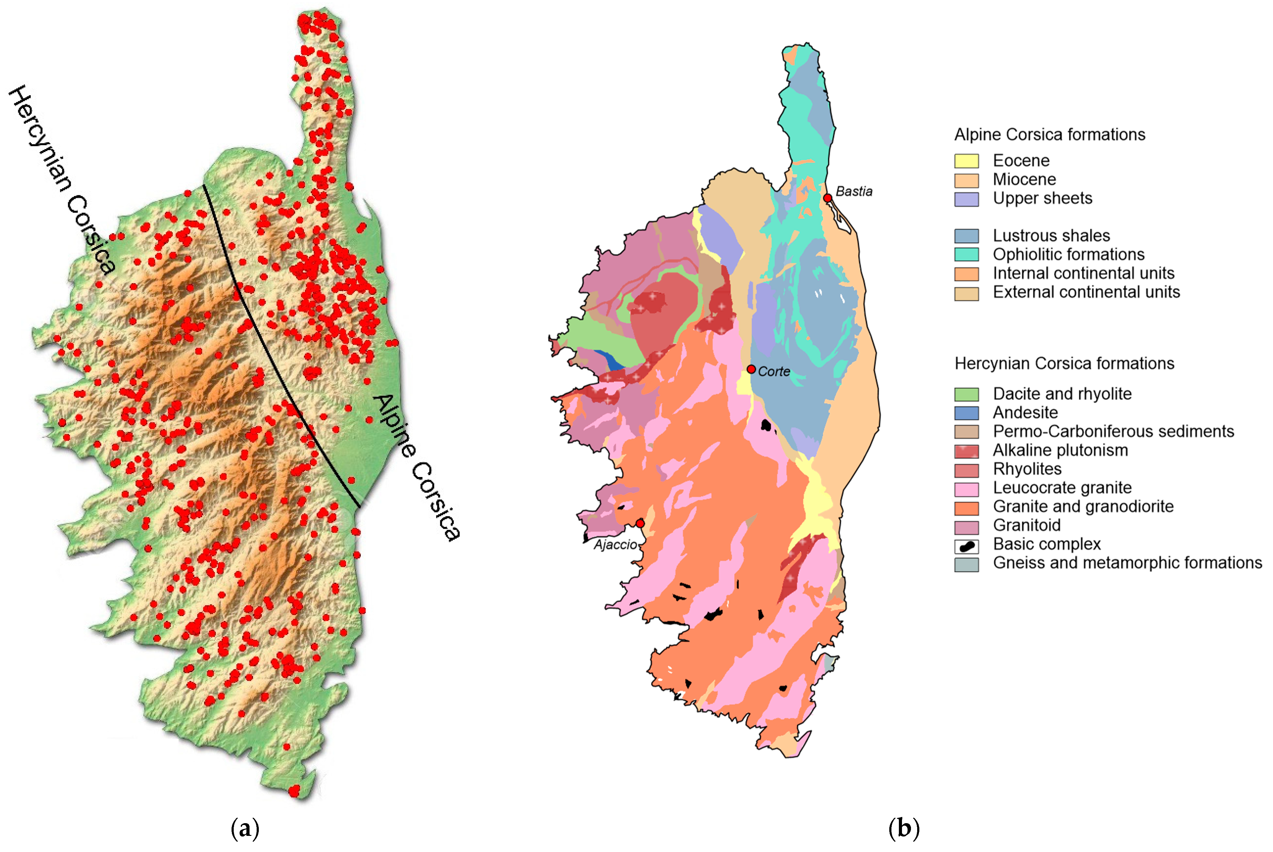
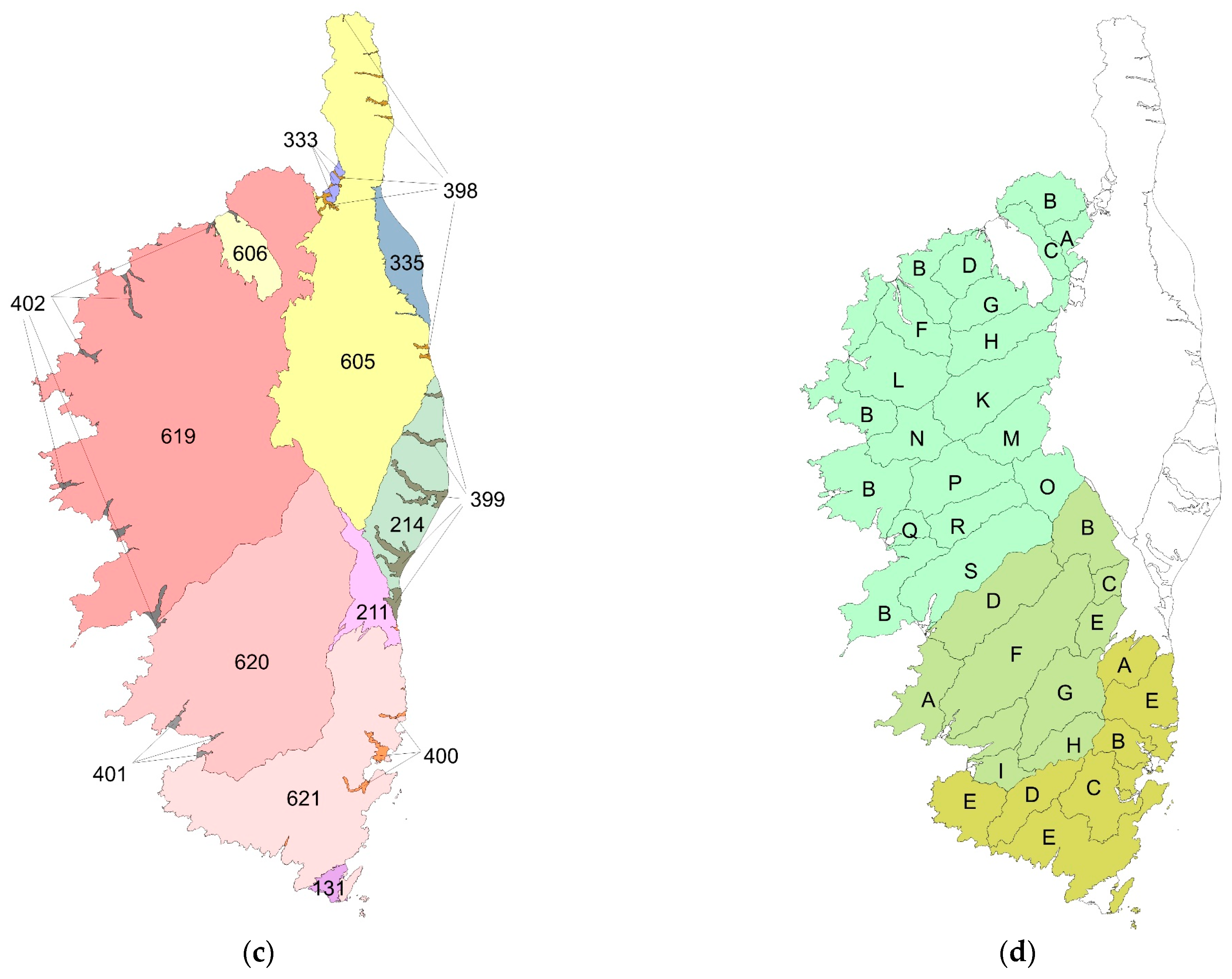
2.1. Corsica Island

The island of Corsica in the Mediterranean Sea (Figure 1a), often referred to as the mountain in the sea, is a mountainous massif 180 km long along the north–south axis and 82 km at its widest, with a total surface area of 8722 km2. The average altitude is 568 m, rising to 2706 (Monte Cinto), with many peaks over 2000 m. The steep gradients and very pronounced relief mean that the area is highly differentiated according to catchment area. From a geological point of view (Figure 1b), the island is clearly structured, with the “Hercynian Corsica” to the west, an essentially crystalline complex composed mainly of granodiorites and monzogranites, alkaline granites and volcanic formations to the north-west, but also a basic tholeiitic complex [23]. The east of the island, generally referred to as “Alpine Corsica”, is occupied by metamorphic formations, particularly schists. Carbonate-quartz sedimentary formations are found in the extreme south of the island. In the French reference system for groundwater bodies (https://services.sandre.eaufrance.fr/geo/sandre, accessed on 7 February 2022), groundwater bodies are referenced by a unique code such as FREGxxx, where FR refers to France, E denotes the Corsica Island and G refers to groundwater resource. In this frame, crystalline Corsica has been divided into three large GWBs, namely FREG619, FREG620 and FREG621, while the smaller Alpine Corsica region is covered by 11 GWBs. The sedimentary part of the extreme south comprises a single GWB (FREG131) (Figure 1c). Given the disproportion in size between the GWBs delineated within the crystalline and alpine regions of Corsica, the three GWBs of the crystalline region were subdivided into sub-GWBs on the basis of hydrographic basins using the island’s DTM (Figure 1d). The aim was to take better account of lithological variability within the crystalline region. The GWBs of the FREG619, FREG620 and FREG621 crystalline regions were therefore subdivided into 15, 8 and 5 sub-GWBs, respectively.

2.2. Sise-Eaux Database Extraction

The Sise-Eaux database (https://data.eaufrance.fr/concept/sise-eaux accessed on 15 March 2021) is supplied with the results of health inspections of water points supplying local communities [24,25]. It covers both untreated water, taken from catchment areas or boreholes, and treated water, i.e., disinfected by chlorination or another process and possibly decanted or filtered. In this work, only untreated (bulk) water has been considered. For each water sample taken, several analysis reports could have been realized, namely, complete with several hundreds of parameters, standard with about 30 parameters, or a routine follow-up, with only about ten parameters. Thus, data extraction from the whole island over 27 years (from April 1993 to September 2020) results in a matrix with a total of 5395 water analyses involving 23 parameters, but with some empty cells that need to be conditioned before processing (Figure 1a). After the manual correction of errors during data entry in the database and the elimination of empty cells, a full matrix consisting of 2830 observations and 15 parameters was used for this study. The 15 parameters selected are major ions (Ca, Mg, Na, SO4, Cl, HCO3), electrical conductivity (EC), bacteriological parameters (total Coliforms (Col.), revivable aerobic bacteria at 22 °C and 37 °C (Aer.22, Aer.37), also including the fecal contamination parameters Enterococci and Escherichia coli (Ent., E. coli), nitrate ions (NO3), and two trace metals (Fe and Mn). For some sampling points, the geographical coordinates were not entered in the database. These coordinates were retrieved from the Infoterre database of the French Geological Survey (https://infoterre.brgm.fr/ accessed on 15 March 2021). Each water sample was then assigned to a GWB, or sub-GWB for the crystalline region, based on its geographic coordinates and depth. Ultimately, these 2830 water samples came from 662 sampling points, i.e., an average of 4.3 samples for each sampling point, and spread over 40 (sub-)GWBs (Figure 1d).

2.3. Data Treatments

The Kolmogorov–Smirnov normality test, which is adapted to high-dimensional statistical distributions [26], was applied to compare the empirical cumulative distribution function to a specified normal distribution, in this case one with the same mean and standard deviation. Following this test, the next step was to perform a logarithmic conditioning of the data as suggested by Jabrane et al. [20], according to the formula: y = log(x + DL), x being the value of the physico-chemical or bacteriological parameter X, and DL the detection limit of this same parameter. The aim of this transformation was to bring the distributions of each parameter closer to a normal distribution and to limit the weight of extreme values likely to obscure certain processes responsible for the variability within the dataset [22,27]. The normality tests revealed the presence of two observations (out of 2830) which clearly showed a data entry error. These two observations were therefore removed from the study.
A principal component analysis (PCA) was then performed on the log-transformed data to reduce the dimensionality of the data hyperspace [19,28] and to identify and rank the sources of variability in the dataset [29]. The PCA was based on the correlation matrix and thus considered the reduced centered variables, which allowed the integration of parameters of very diverse natures and units. Furthermore, it was carried out by diagonalization of the correlation matrix. Under this condition, the factorial axes were perpendicular to each other, and were therefore theoretically associated with independent processes responsible for the variability of water quality. The factorial axes, totaling about 95% of the information, were retained. The last factorial axes, explaining a small percentage of the variance, and generally considered as statistical noise [30], were eliminated. The reduction in dimensionality was estimated using the Bartlett sphericity test [31].
The mean values of the coordinates of each GWB (and sub-GWB) on each factorial axis were then calculated, thus characterizing each of these hydrogeological units. An unsupervised ascending hierarchical clustering (UHC) was then used to classify the hydrogeological units by degree of similarity, all parameters considered. The result is a group of GWBs containing GWBs with similar groundwater quality. By way of comparison, this process was carried out by considering only the GWBs delineated by the French Geologic Survey, i.e., with only three GWBs covering the entire crystalline region of the island, and then subdividing this region into sub-GWBs. At this stage, its sampling point, the GWB or sub-GWB, and the group of GWBs and sub-GWBs to which it belongs characterize each water sample. The choice of the number of groups was guided by the variation of the ratio between the inter-group and intra-group variability in order to maximize the intra-group homogeneity and the inter-group heterogeneity. The results are iteratively collated to produce a dendrogram. The choice of where to cut the phenom line was determined by a compromise between, on the one hand, the break in the slope in the relationship between the number of clusters and dissimilarity, and on the other hand, the requirements in terms of managing the number of spatial units generated. Indeed, too many space units would be unmanageable in terms of monitoring and protection by the health agency.
Finally, an analysis of variance (ANOVA) was carried out to measure the variance at each grouping scale using the R2 coefficient, which is the ratio between the inter-class variance, i.e., the variance explained, and the total variance [32,33]. This analysis measures the effectiveness of the hydrogeological unit grouping method chosen by measuring the loss of information during grouping from the sampling point scale to the (sub)GWB groups [22]. The variance explained at the sampling point scale indicates the spatial variability at this scale, and the deviation of the R2 from unity indicates the variance linked to temporal variability (since there are on average 4.3 samples per sampling point), added to a variability linked to analytical imprecision deemed negligible. The loss of information accompanying clustering was measured by the R2 value indicating the spatial variability at each nested scale subGWB, GWB, subGWB group and GWB group.

3. Results

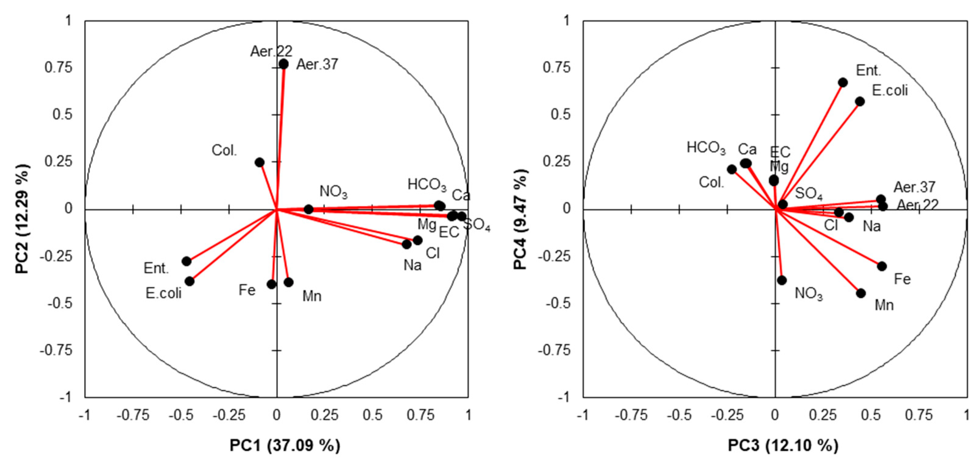
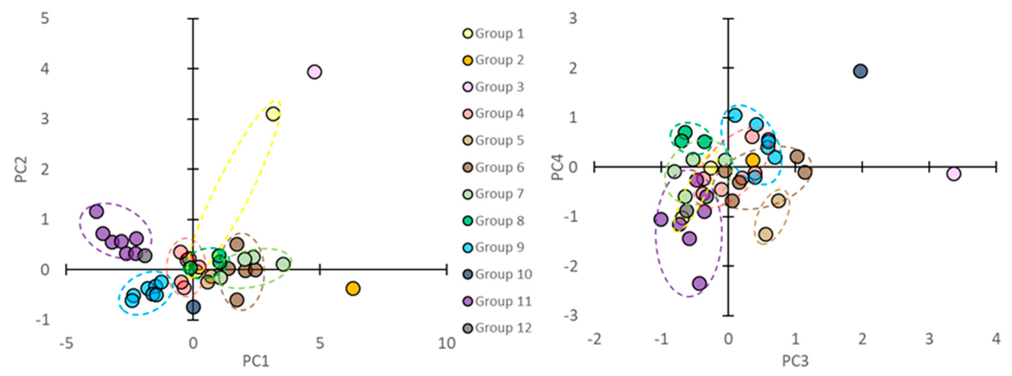
3.1. Principal Component Analysis

The distribution of the inertia of the different factorial axes is shown in Table 1. PCA allowed a significant reduction in dimensionality. The first principal component clearly stood out from the others, accounting for 37.1% of the total variance. About half of the information contained in the database (49.3%) was concentrated in the first factorial plan, which is substantial compared with the 15 parameters in the dataset. The first five factorial axes had eigenvalues greater than unity, meaning that they concentrated more information than a single parameter [29]. The first eight axes, which accounted for 94.7% of the information, were retained for further hierarchical clustering calculations. The remaining 5.3% was considered as statistical noise and information generated by minor sources of variability.
The contribution of the parameters to the first four PCs is shown in Figure 2. The first factorial axis explained 37.1% of the variance and contrasted mineralized water, positively scored with CE and major ions (Ca, Mg, Na, Cl, SO4, HCO3), with poorly mineralized water contaminated by E. coli and Enterococcus. The second factorial axis (12.3% of the variance) contrasted water marked by revivable bacteria with water with a chloride-sodium chemical profile marked by the presence of metals and fecal contamination. The third PC (12.1% of the variance) was also affected by the presence of revivable bacteria but also fecal contamination (E. coli and Ent.) and the presence of metals, again in a predominantly sodium chloride chemical context, while the fourth PC had positive coordinates for fecal contamination but negative for metals. Bartlett’s sphericity test showed a calculated X2 of 40143, much stronger than the critical X2 (=130, significance level of 0.05 and p-value < 0.0001), which highlighted the fact that the switch from 15 initial parameters to eight retained PCs, i.e., an eight-dimensional hyperspace, was a significant dimensional contraction with a loss of only 5.3% of the information.

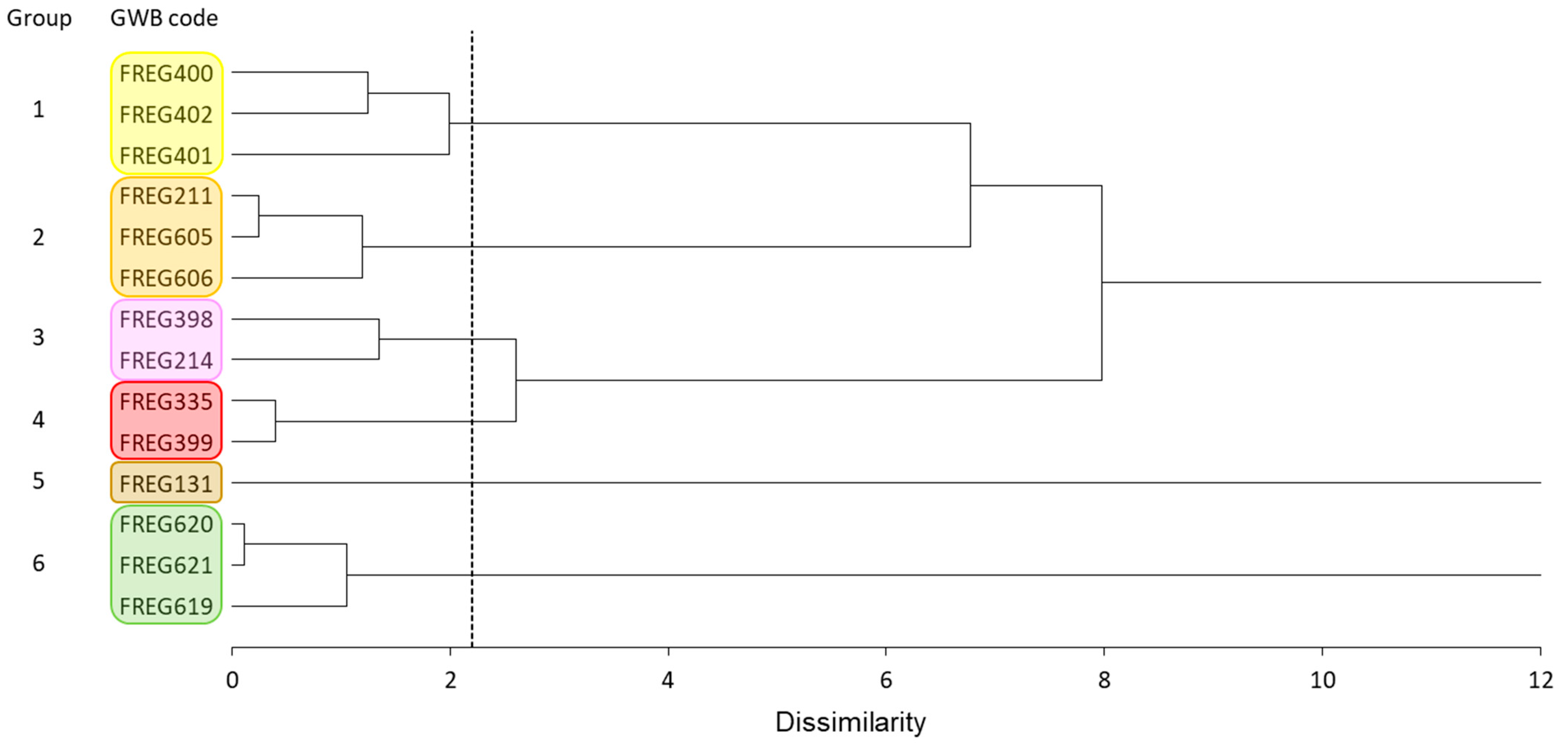
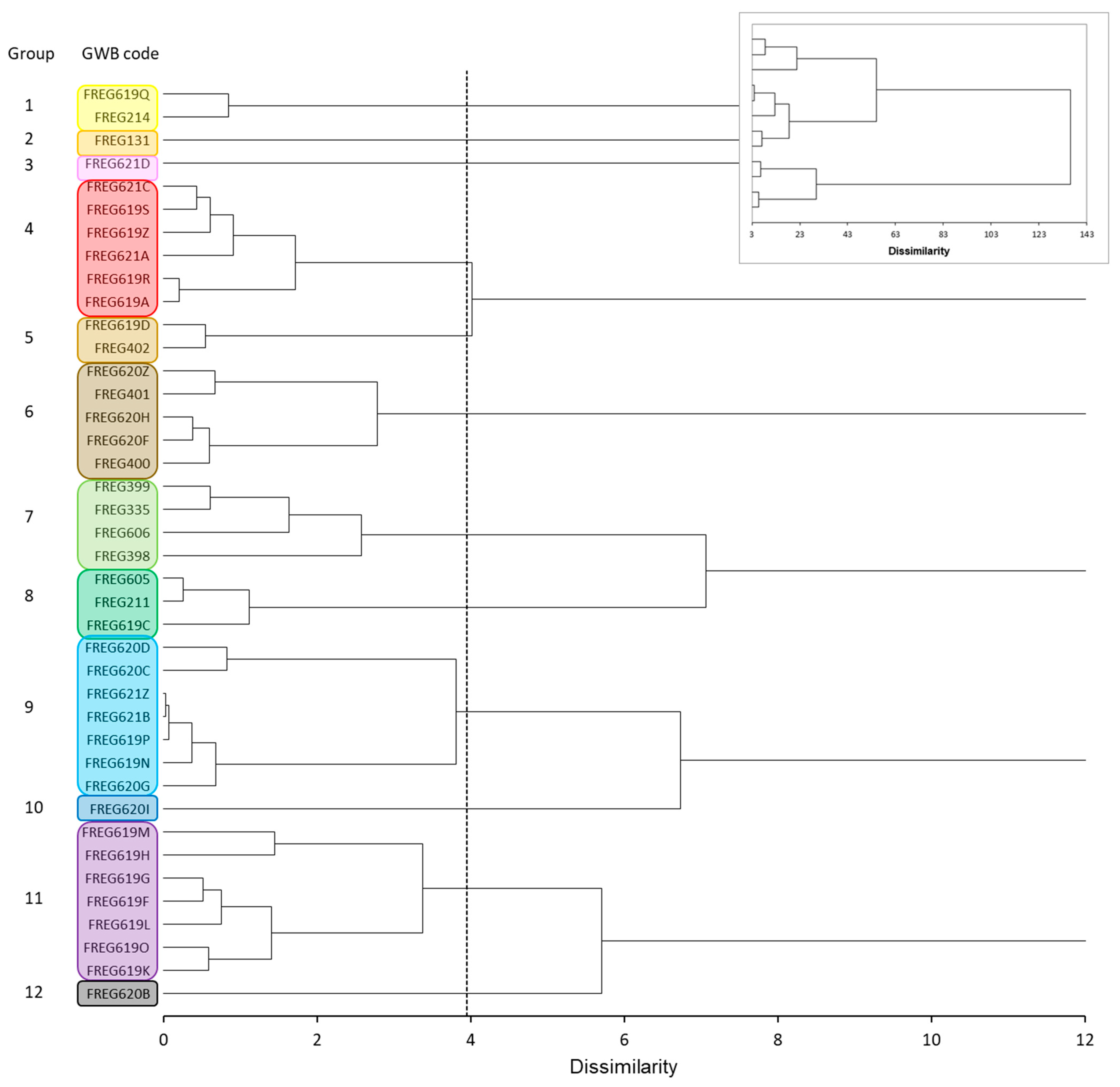
3.2. Unsupervised Agglomerative Hierarchical Clustering

The clustering diagrams obtained from the first eight factorial axes for the 15 GWBs and the 40 GWBs + sub-GWBs are shown in Figure 3 and Figure 4, respectively. The GWB coded FREG333, for which there were few water analyses, was withdrawn from the study at this clustering stage. Clustering of the GWBs reveals six groups of GWBs. The distribution of these groups highlights an opposition between crystalline Corsica, which constitutes a large undifferentiated group covering approximately two thirds of the island, and the rest of the territory (Figure 5a).
By subdividing the GWBs of the crystalline region, we obtained 40 units over the whole of the island, and the hierarchical classification resulted in 12 distinct groups, the distribution of which is presented in Figure 5b. This classification has lessened the diversity of waters within Alpine Corsica, with several previously distinct GWBs now grouped together in group 8. On the other hand, a diversity of waters appeared within the crystalline region of the Hercynian Corsica, with sub-GWBs grouped together in small patches (groups 5, 6 and 11) or dispersed (groups 3, 4, 7, 9). Some sub-GWBs stood out from the others, such as the GWB in the sedimentary material at the southern extremity of the island (group 2) and two sub-GWBs from FREG620, which formed groups 10 and 12.
The distribution of the groups obtained in the PC1-PC2 and PC3-PC4 score plots is shown in Figure 6, and the mean values of the parameters for each group are summarized in Table 2.
Groups 9 and 10, located on crystalline rocks in Hercynian Corsica, showed the highest levels of fecal contamination. Group 10 comprises a single sub-GWB, reflecting a local specificity. It had the same characteristics as group 9, but differed in that it contained an abundance of revivable bacteria and even higher levels of E. coli contamination than group 9. Both groups 9 and 10 are located in the same geographical environment, i.e., mountainous areas, and therefore sloping, on granite, leucocratic granite and granodiorite. All these factors (altitude, slope, erosion, shallow soils) are even more marked in groups 11 and 12, which correspond to high mountain areas (Monte Cinto, Monte Corona) and ridge lines (Marmano and Pietra Piana forests) with skeletal or even absent soils. Group 11 is located on a more acidic lithology of rhyolites and alkaline plutonism. In contrast, group 2, the only small area in Corsica on limestone (FREG131), is characterized by very low fecal contamination and higher mineral load. Group 3, also made up of a single sub-GWB (FREG621D) on granite, corresponds to a wide, low-altitude, non-wooded valley.

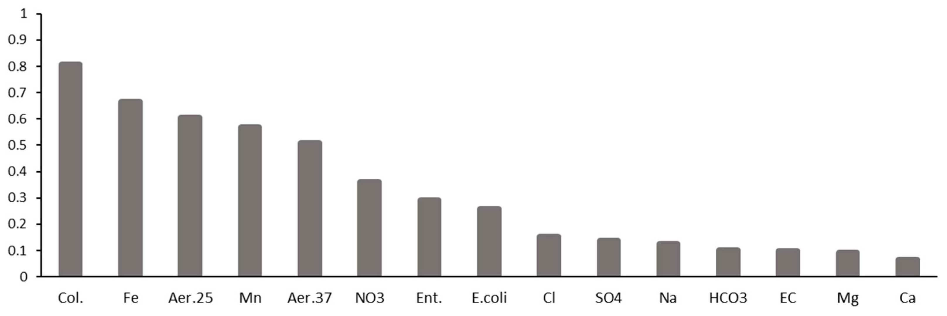
3.3. Explained Variance Measured from R2

The temporal variability for each parameter is shown in Figure 7. This was low for major ions and electrical conductivity, intermediate for fecal contamination parameters (E. coli and Ent.) and nitrates, and high for coliform parameters, revivable bacteria and metals. As a result, the proportion of spatial variability for the latter was reduced. The spatial variance explained for each parameter according to the level of grouping scale is displayed in Table 3, together with the corresponding numbers. All the results were related to the spatial variability at the scale of the collection points.
Grouping the GWBs into 40 units, i.e., considering the GWBs combined with the sub-GWBs of the crystalline region, resulted in a fairly significant reduction in the variance explained, mainly for bacteriological parameters and metals, less marked for nitrates, and even less for fecal contamination parameters and major ions. Grouping into the 15GWBs delineated by the French Geological Survey, or into 12 groups of (sub-)GWBs, was accompanied by a slight additional reduction in the explained variance. However, for most parameters, grouping into 12 units resulted in a higher proportion of explained variance than grouping into 15 units.

4. Discussion

4.1. A multifactorial Information Set

The distribution of the PC inertia, and in particular the fact that the first five eigenvalues are greater than unity, underlines that the information contained in the dataset cannot be summed up in one or two parameters, but on the contrary that this information is clearly multifactorial. The contrast between mineralized water and water with low mineral content but subject to fecal contamination (E. coli and Enterococci) has been classically observed in the processing of databases in Mediterranean climates [18,19,20,21,22]. During rainy periods, run-off water, which is poorly mineralized but turbid and loaded with bacteria, contaminates vulnerable or poorly protected water catchment structures. In contrast, during low-water periods, the catchment structures only collect groundwater, which is more mineralized, filtered by the soil and less affected by surface bacterial contamination. This interpretation is consistent with the high temporal variability of bacteriological parameters (Figure 7). However, the high contribution of fecal contamination parameters on the first four principal components suggests a more complex determinism of the spatial and temporal variations in these parameters. As the factorial axes are orthogonal in the hyperspace of the data, they cannot reflect correlated mechanisms, and each PC represents a process that is independent of the others. The pathways of fecal contamination cannot therefore be reduced solely to runoff induced by heavy rainfall, but are a priori the result of a diversity of pathways, as has already been suggested for other regions [19]. The factors are multiple and interdependent, with environmental factors influencing the presence or absence of extensive livestock farming (particularly pigs), which should contribute to this result.

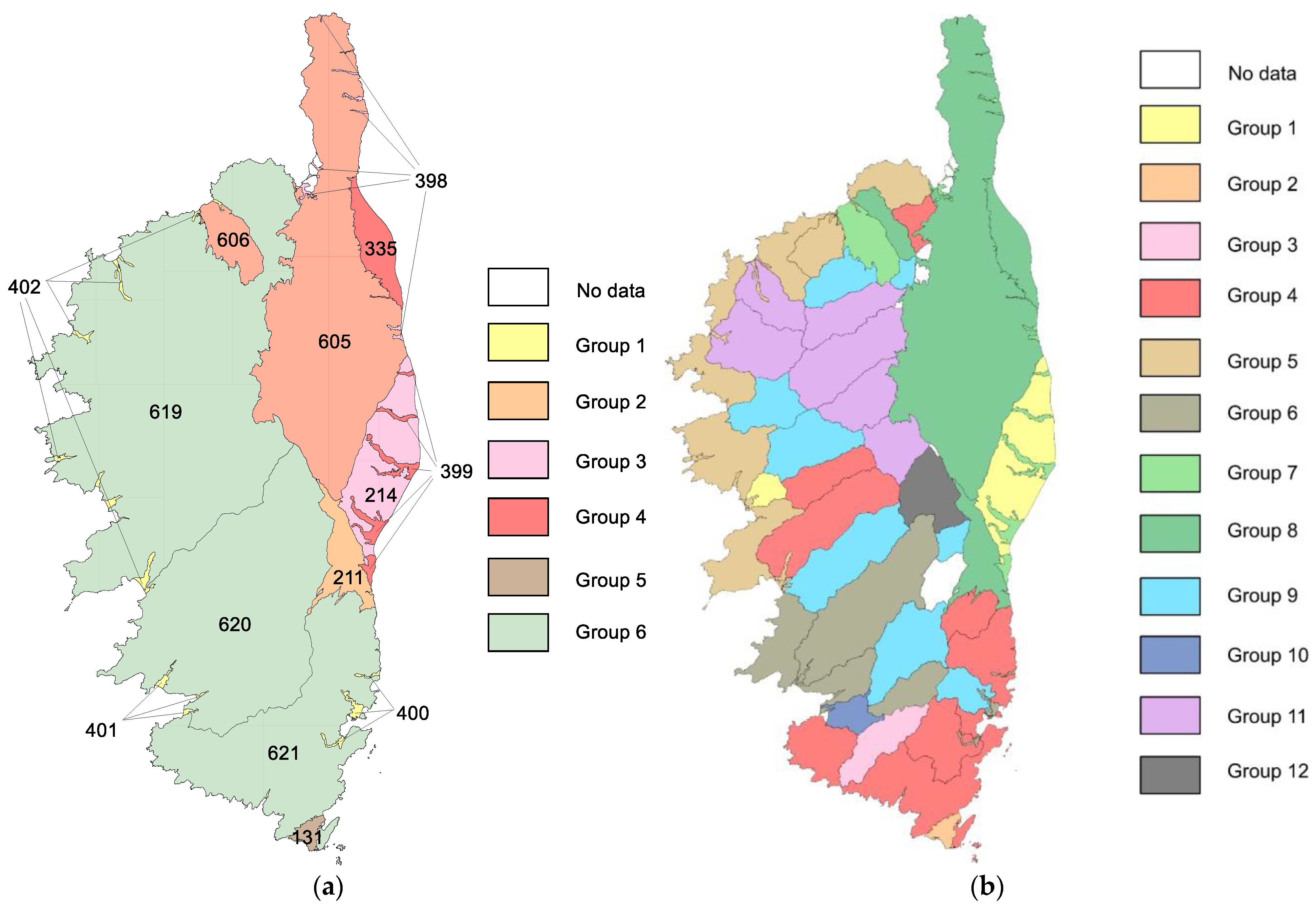
4.2. A Sub-GWB Division Better Suited to Monitoring the Resource

The large undifferentiated group of GWBs covering the crystalline region (Figure 5a) contrasts with the medium to very small groups in the other regions. This highlights the significant disparity in terms of the area covered by the different GWB groups. The effectiveness of a mapping can be measured by the variance explained for a given number of spatial units. For the same number of units, the most relevant map containing the most spatial information is the one with the highest explained variance. In our case, the 15 GWBs (Figure 1c) convey less information than 12 groups of sub-GWBs (Figure 5b) without leading to an increase in the number of spatial units. The division of the territory into GWBs proposed by the French Geological Survey on the basis of structural geology is therefore less effective than the map of sub-GWB groups in terms of groundwater quality. This result is difficult to reconcile with the development of a strategy for monitoring and protecting water resources intended for human consumption. The size of the crystalline region and its division into three GWBs makes it impossible to distinguish the lithological variability within this zone, and to visualize the resulting variability in water quality. Such a division will necessarily lead to monitoring of the crystalline region that is ill suited to the diversity of the waters in this region. The GWB’s classification into six groups, based largely on the island’s structural geology, is disappointing: it is relevant, but trivial and too schematic for the zonation of Corsican groundwater. Crystalline Corsica has highly variable rock types, particularly in terms of alkali and earth alkali content. This means that the chemical composition of the water, the nature of the soil, the physico-chemical properties of the surface formations, and the susceptibility to erosion and the transport of bacteria are all very different depending on the lithology.
This result quantifies and demonstrates (1) the need to divide large GWBs into sub-GWBs and (2) the effectiveness of grouping sub-GWBs, which ultimately corresponds to a gain in information compared with dividing into 15 units, for most parameters, particularly for fecal contamination criteria, revivable bacteria, most major ions and electrical conductivity. Only the parameters Ca, HCO3 and NO3 do not follow this rule, but the low proportion of spatial variability partly explains this result for nitrates. This result, which is valid for almost all the parameters, demonstrates the relevance and interest of working on the scale of groups of sub-GWBs and justifies, a posteriori, the approach of dividing the three GWBs of the crystalline region. This better score for dividing the area into groups of sub-GWBs is probably not due to the fact of having chosen a topographical criterion for dividing crystalline Corsica, i.e., the river basins, but rather to the fact of indirectly integrating the lithological heterogeneity internal to crystalline Corsica, even if this choice can be partially justified by the impact on likely flow paths. In hindsight, it turns out that this division into basins reflects the lithology of crystalline Corsica quite well (compare, for example, Figure 1b,d, or Figure 1b and Figure 5b). If we had chosen to focus directly on lithology, our results would probably have been just as good. This choice is valid for Corsica, but is not necessarily applicable to other sites.

4.3. A Result Closer to the Distribution of Lithology

The clustering result from the GWBs (Figure 5a) is in line with the structural geology of Corsica, since it is on this basis that the GWBs were delimited, whereas the clustering of the sub-GWBs (Figure 5b) gives a result close to the petrographic distribution, and thus seems to correspond to the reality of another geological information. This result makes sense. Within crystalline Corsica, the granitoid zones near the north-west coast are clearly differentiated in terms of water quality (group 5). Similarly, the areas of alkaline plutonism and rhyolites (group 11) stand out clearly from the granite and granodiorite areas (groups 4, 6 and 9).

4.4. Other Environmental Factors

Steep slopes and siliceous rock with a low alkaline and alkali-earth content result in very coarse-textured soils with a relatively low calcium level, which reduces the flocculation of colloids and facilitates the transfer of suspended matter, the main vector for the transport of bacteria. This explains the high level of fecal contamination in groups 9 and 10. The altitude and steep slopes also favor short-lived water-rock interaction and cooler temperatures, resulting in water with a low mineral content, which is very marked in groups 9 and 10, and even more so in groups 11 and 12. In contrast, group 2, which is on limestone and therefore rich in calcium, is more gently sloping and is characterized by very low fecal contamination, probably due to the flocculating role of calcium ions, the reduction in run-off (two major factors in solid and therefore bacterial transport), and a slow flow in the aquifer that encourages the self-purification process and the elimination of pollution. The limestone lithology, a relatively soluble rock, explains the higher mineral content. For group 3, with its fairly flat topography on granite, run-off is reduced and the soils are thicker, which limits fecal contamination, which is lower than in the surrounding units. At the same time, the shallower topography favors slower run-off and longer water–rock interaction times, resulting in a higher mineral content than in other areas of crystalline Corsica. In conclusion, lithological specificity not only affects the composition of water in terms of major ions. The relative abundance of alkaline earths or alkalis in the less siliceous lithologies probably results in greater structural stability in the soils derived from them, and consequently less vulnerability to bacterial transport, which may explain this differentiation in multi-parameter water quality between the different formations of crystalline Corsica.
To sum up, the division of the GWBs of the crystalline region into sub-GWBs has led to a better understanding of the diversity of waters, by revealing the role of:
  • The nature of the soils, an important factor in the vulnerability of water catchment structures;
  • The altitude, which has an impact on temperature and therefore on human land use, the type of forest, the intensity of pedogenesis, etc.;
  • The geomorphology;
  • The lithological diversity within the crystalline region, with an important aspect regarding the presence of flocculent cations.
While remaining on this purely lithological criterion, it appears that it would be relevant to distinguish zones with alkaline plutonism from granitic zones. The results of the study show that it would be possible to review the division of GWBs, particularly in crystalline Corsica.

4.5. Methodological Contribution

The present work highlights a series of methodological advances that we feel are relevant to bring together here:
  • The study confirms that the method implemented, and progressively improved, is suitable for highlighting the information contained in Sise-Eaux type databases. Of course, the existence of such a database is a prerequisite for its application;
  • Quantifying the loss of information that accompanies the grouping of GWBs makes it possible to measure the effectiveness of the method.
  • This analysis method, developed for vast regions of the order of 60,000 to 80,000 km2, can be deployed for regions around 10 times smaller, even if the European Commission recommends an even larger scale, that of the major European watersheds (Danube, Rhône, Rhine, Seine, Loire, Po, etc.);
  • While it now appears that the information analysis method can be extended to other administrative regions, we do not know whether it can be extended to new parameters not taken into account here (pesticides, land use, fractured medium, water–rock contact time, etc.). The use of databases of much larger dimensions is currently being tested in the Provence-Alpes-Côte d’Azur administrative region (PACA, France);
  • However, the proposed method has certain limitations. In particular, at this stage, the analysis is carried out parameter by parameter, which does not take into account the interrelations between several parameters. Access to a greater number of parameters over a larger number of observations should make it possible to establish a typology of parameter behaviour, while separating their variability in space (range of each variable) and in time (common variability of parameters during rainy events, more or less marked seasons, or even multi-annual dry or wet periods). This typology of parameters would be a further step forward in the type of information extracted from large databases.

5. Conclusions

A method for mapping groundwater quality in France has been developed by our research group over the last few years, with the aim of optimizing the surveillance and monitoring of groundwater quality by regional health agencies. As the method has been applied to areas of varying size (Provence-Alpes-Côte d’Azur and Occitanie regions), it has become increasingly effective. Here, the method has been tested in the case of a much smaller region, the island of Corsica, and its application on the basis of GWBs delineated by the French Geologic Survey gives relevant but trivial results, which do not allow discerning of the variability of water quality within Hercynian crystalline Corsica. An adaptation is proposed. It consists of dividing the large GWBs of crystalline Corsica into sub-GWBs on the basis of hydrographic basins. Our study shows that it is possible, using analysis of variance, to quantify the evolution of the loss of spatial information when changes of scale are made, from the sampling point to the various groupings of GWBs. The analysis of variance shows a gain in information despite a smaller number of spatial units, which can be explained by a better consideration of the spatial variability of groundwater quality within the crystalline region. The results obtained should serve as the starting point for a revision of the GWBs for the island of Corsica based on groundwater quality, but also on lithology. As things stand at present, very small lithological units have been taken into account, and rightly so, in drawing up the GWBs, because of their specific nature. The calculation of groups of GWBs or sub-GWBs has confirmed their specificity, but they represent extremely small areas. On the other hand, the internal variability of the lithological units, which are much more extensive within crystalline Corsica, has not been taken into account, which could prove useful, particularly for health agencies, in developing a strategy for monitoring the quality of groundwater resources.

Author Contributions

Conceptualization, H.L., V.V. and I.K.; methodology, H.L., V.V. and L.B.; software, V.V. and I.M.; validation, A.T., M.A., I.M. and H.L.; formal analysis, H.L., V.V. and L.B.; investigation, H.L.; resources, É.G., F.H. and C.M.; data curation, A.-A.B., L.B. and I.M.; writing—original draft preparation, H.L. and V.V.; writing—review and editing, L.B.; visualization, L.B. and I.M.; supervision, I.K. and V.V.; project administration, I.K. All authors have read and agreed to the published version of the manuscript.

Funding

This research received no external funding.

Data Availability Statement

The data in this study are the property of Corsica Regional Health Agency and are included in the SISE-Eaux French database.

Acknowledgments

The authors would like to thank Patrice Grandjean (Corsica Regional Health Agency) for his help with data extraction.

Conflicts of Interest

The authors declare no conflict of interest.

References

  1. Walker, D.B.; Baumgartner, D.J.; Gerba, C.P.; Fitzsimmons, K. Chapter 16—Surface Water Pollution. In Environmental and Pollution Science, 3rd ed.; Brusseau, M.L., Pepper, I.L., Gerba, C.P.B.T.-E., Eds.; Academic Press: Cambridge, MA, USA, 2019; pp. 261–292. ISBN 978-0-12-814719-1. [Google Scholar]
  2. Li, P.; Karunanidhi, D.; Subramani, T.; Srinivasamoorthy, K. Sources and Consequences of Groundwater Contamination. Arch. Environ. Contam. Toxicol. 2021, 80, 1–10. [Google Scholar] [CrossRef] [PubMed]
  3. Woldt, W.; Bogardi, I. Ground water monitoring network design using multiple criteria decision making and geostatistics. JAWRA J. Am. Water Resour. Assoc. 1992, 28, 45–62. [Google Scholar] [CrossRef]
  4. Hudak, P.F.; Loaiciga, H.A. An optimization method for monitoring network design in multilayered groundwater flow systems. Water Resour. Res. 1993, 29, 2835–2845. [Google Scholar] [CrossRef]
  5. Frapporti, G.; Hoogendoorn, J.H.; Vriend, S.P. Detailed Hydrochemical Studies as a Useful Extension of National Ground-Water Monitoring Networks. Groundwater 1995, 33, 817–828. [Google Scholar] [CrossRef]
  6. Meyer, P.D.; Brill, E.D., Jr. A method for locating wells in a groundwater monitoring network under conditions of uncertainty. Water Resour. Res. 1988, 24, 1277–1282. [Google Scholar] [CrossRef]
  7. Lee, J.-Y.; Yi, M.-J.; Yoo, Y.-K.; Ahn, K.-H.; Kim, G.-B.; Won, J.-H. A review of the National Groundwater Monitoring Network in Korea. Hydrol. Process. 2007, 21, 907–919. [Google Scholar] [CrossRef]
  8. Esquivel, J.M.; Morales, G.P.; Esteller, M.V. Groundwater Monitoring Network Design Using GIS and Multicriteria Analysis. Water Resour. Manag. 2015, 29, 3175–3194. [Google Scholar] [CrossRef]
  9. European Commission Directive 2006/118/EC of the European Parliament and of the Council of 12 December 2006 on the protection of groundwater against pollution and deterioration. Off. J. Eur. Union 2006, 372, 19–31.
  10. Allan, I.J.; Vrana, B.; Greenwood, R.; Mills, G.A.; Knutsson, J.; Holmberg, A.; Guigues, N.; Fouillac, A.-M.; Laschi, S. Strategic monitoring for the European Water Framework Directive. TrAC Trends Anal. Chem. 2006, 25, 704–715. [Google Scholar] [CrossRef]
  11. Martínez-Navarrete, C.; Jiménez-Madrid, A.; Sánchez-Navarro, I.; Carrasco-Cantos, F.; Moreno-Merino, L. Conceptual Framework for Protecting Groundwater Quality. Int. J. Water Resour. Dev. 2011, 27, 227–243. [Google Scholar] [CrossRef]
  12. Masciale, R.; Amalfitano, S.; Frollini, E.; Ghergo, S.; Melita, M.; Parrone, D.; Preziosi, E.; Vurro, M.; Zoppini, A.; Passarella, G. Assessing Natural Background Levels in the Groundwater Bodies of the Apulia Region (Southern Italy). Water 2021, 13, 958. [Google Scholar] [CrossRef]
  13. Frollini, E.; Preziosi, E.; Calace, N.; Guerra, M.; Guyennon, N.; Marcaccio, M.; Menichetti, S.; Romano, E.; Ghergo, S. Groundwater quality trend and trend reversal assessment in the European Water Framework Directive context: An example with nitrates in Italy. Environ. Sci. Pollut. Res. 2021, 28, 22092–22104. [Google Scholar] [CrossRef]
  14. Goldscheider, N. Karst groundwater vulnerability mapping: Application of a new method in the Swabian Alb, Germany. Hydrogeol. J. 2005, 13, 555–564. [Google Scholar] [CrossRef]
  15. Raihan, A.T.; Bauer, S.; Mukhopadhaya, S. An AHP based approach to forecast groundwater level at potential recharge zones of Uckermark District, Brandenburg, Germany. Sci. Rep. 2022, 12, 6365. [Google Scholar] [CrossRef]
  16. Flindt Jørgensen, L.; Villholth, K.G.; Refsgaard, J.C. Groundwater management and protection in Denmark: A review of pre-conditions, advances and challenges. Int. J. Water Resour. Dev. 2017, 33, 868–889. [Google Scholar] [CrossRef]
  17. Masses d’eau Souterraines-Métropole-Version État Des Lieux. 2019. Available online: https://geo.data.gouv.fr/fr/datasets/1a983edfe5ea441fef359a652e98217c9c3ce3c6 (accessed on 10 November 2023).
  18. Tiouiouine, A.; Jabrane, M.; Kacimi, I.; Morarech, M.; Bouramtane, T.; Bahaj, T.; Yameogo, S.; Rezende-Filho, A.; Dassonville, F.; Moulin, M.; et al. Determining the relevant scale to analyze the quality of regional groundwater resources while combining groundwater bodies, physicochemical and biological databases in southeastern france. Water 2020, 12, 3476. [Google Scholar] [CrossRef]
  19. Tiouiouine, A.; Yameogo, S.; Valles, V.; Barbiero, L.; Dassonville, F.; Moulin, M.; Bouramtane, T.; Bahaj, T.; Morarech, M.; Kacimi, I. Dimension reduction and analysis of a 10-year physicochemical and biological water database applied to water resources intended for human consumption in the provence-alpes-cote d’azur region, France. Water 2020, 12, 525. [Google Scholar] [CrossRef]
  20. Jabrane, M.; Touiouine, A.; Bouabdli, A.; Chakiri, S.; Mohsine, I.; Valles, V.; Barbiero, L. Data Conditioning Modes for the Study of Groundwater Resource Quality Using a Large Physico-Chemical and Bacteriological Database, Occitanie Region, France. Water 2023, 15, 84. [Google Scholar] [CrossRef]
  21. Jabrane, M.; Touiouine, A.; Valles, V.; Bouabdli, A.; Chakiri, S.; Mohsine, I.; El Jarjini, Y.; Morarech, M.; Duran, Y.; Barbiero, L. Search for a Relevant Scale to Optimize the Quality Monitoring of Groundwater Bodies in the Occitanie Region (France). Hydrology 2023, 10, 89. [Google Scholar] [CrossRef]
  22. Mohsine, I.; Kacimi, I.; Abraham, S.; Valles, V.; Barbiero, L.; Dassonville, F.; Bahaj, T.; Kassou, N.; Touiouine, A.; Jabrane, M.; et al. Exploring Multiscale Variability in Groundwater Quality: A Comparative Analysis of Spatial and Temporal Patterns via Clustering. Water 2023, 15, 1603. [Google Scholar] [CrossRef]
  23. De Graciansky, P.-C.; Roberts, D.G.; Tricart, P. Chapter Nine—The Tethyan Margin in Corsica. In The Western Alps, from Rift to Passive Margin to Orogenic Belt; De Graciansky, P.-C., Roberts, D.G., Tricart, P., Eds.; Elsevier: Amsterdam, The Netherlands, 2011; Volume 14, pp. 183–188. ISBN 0928-2025. [Google Scholar]
  24. Chery, L.; Laurent, A.; Vincent, B.; Tracol, R. Echanges SISE-Eaux/ADES: Identification Des Protocoles Compatibles Avec Les Scénarios D’échange SANDRE; ONEMA: Vincennes/Orléans, France, 2011. [Google Scholar]
  25. Gran-Aymeric, L. Un portail national sur la qualite des eaux destinees a la consommation humaine. Tech. Sci. Méthodes 2010, 12, 45–48. [Google Scholar] [CrossRef]
  26. Steinskog, D.J.; Tjøstheim, D.B.; Kvamstø, N.G. A Cautionary Note on the Use of the Kolmogorov–Smirnov Test for Normality. Mon. Weather Rev. 2007, 135, 1151–1157. [Google Scholar] [CrossRef]
  27. Feng, C.; Wang, H.; Lu, N.; Chen, T.; He, H.; Lu, Y.; Tu, X.M. Log-transformation and its implications for data analysis. Shanghai Arch. Psychiatry 2014, 26, 105–109. [Google Scholar] [PubMed]
  28. Barbel-Périneau, A.; Barbiero, L.; Danquigny, C.; Emblanch, C.; Mazzilli, N.; Babic, M.; Simler, R.; Valles, V. Karst flow processes explored through analysis of long-term unsaturated-zone discharge hydrochemistry: A 10-year study in Rustrel, France. Hydrogeol. J. 2019, 27, 1711–1723. [Google Scholar] [CrossRef]
  29. Helena, B.; Pardo, R.; Vega, M.; Barrado, E.; Fernandez, J.M.; Fernandez, L. Temporal evolution of groundwater composition in an alluvial aquifer (Pisuerga River, Spain) by principal component analysis. Water Res. 2000, 34, 807–816. [Google Scholar] [CrossRef]
  30. Rezende Filho, A.; Furian, S.; Victoria, R.; Mascré, C.; Valles, V.; Barbiero, L. Hydrochemical variability at the upper paraguay basin and pantanal wetland. Hydrol. Earth Syst. Sci. 2012, 16, 2723–2737. [Google Scholar] [CrossRef]
  31. Gleser, L.J. A Note on the Sphericity Test. Ann. Math. Stat. 1966, 37, 464–467. [Google Scholar] [CrossRef]
  32. Achen, C.H. What Does “Explained Variance“ Explain?: Reply. Polit. Anal. 1990, 2, 173–184. [Google Scholar] [CrossRef]
  33. Miles, J. R Squared, Adjusted R Squared. In Wiley StatsRef: Statistics Reference Online; Wiley: Hoboken, NJ, USA, 2014; ISBN 9781118445112. [Google Scholar]
Figure 1. (a) Distribution of groundwater sample collection points; (b) main geological formations; (c) compartmentalization of FREG groundwater bodies according to the French Geological Survey; (d) subdivision of the three main groundwater bodies (FREG619, FREG620 and FREG621) of the crystalline region according to river basins.
Hydrology 10 00213 g001aHydrology 10 00213 g001b
Figure 2. Distribution of the parameters on the four first principal components.
Hydrology 10 00213 g002
Figure 3. Dendrogram resulting from the agglomerating hierarchical clustering based on 14 GWB, individualizing six groups of groundwater bodies.
Hydrology 10 00213 g003
Figure 4. Dendrogram resulting from the agglomerating hierarchical clustering, based on 40 GWB and sub-GWB, individualizing 12 groups of groundwater bodies.
Hydrology 10 00213 g004
Figure 5. Distribution of (a) the 6 GWB groups from clustering based on 14 groundwater bodies and (b) the 12 subGWB groups from clustering based on 40 sub-groundwater bodies.
Hydrology 10 00213 g005
Figure 6. Distribution of the 12 sub-GWB groups in the PC1-PC2 and PC3-PC4 score plots.
Hydrology 10 00213 g006
Figure 7. Temporal variance of each water quality parameter within the dataset (2828 water samples collected over 27 years).
Hydrology 10 00213 g007
Table 1. Inertia of the factorial axes of the PCA carried out on 2828 observations and 15 parameters.
PC1PC2PC3PC4PC5PC6PC7
Explained variance %37.112.312.19.586.56
Cumulative explained variance %37.149.461.570.97985.591.5
Eigenvalue5.561.841.821.421.20.980.91
Table 2. Mean values of the parameters for each group of sub-GWBs.
Groups
123456789101112
Ent.0.150.000.000.450.170.320.120.491.121.560.560.08
E. coli0.050.080.000.450.110.390.050.351.202.060.360.11
Col.0.000.000.000.000.020.000.000.090.000.000.120.00
Aer.220.000.000.550.010.020.020.000.010.000.060.010.00
Aer.370.000.000.270.000.020.020.000.010.000.050.010.00
EC2.523.032.752.162.232.402.522.392.002.281.771.93
Ca1.312.111.550.820.921.091.531.440.701.050.460.82
Mg1.041.011.260.550.640.790.990.820.370.720.110.25
Cl1.552.151.901.321.391.571.241.091.121.410.840.83
SO41.281.581.340.820.921.031.120.950.620.860.550.46
Na1.441.881.691.171.211.391.060.890.991.230.740.82
HCO31.912.572.151.491.561.742.172.031.361.701.081.51
NO31.230.870.670.250.290.260.560.150.170.170.35−0.24
Fe1.040.981.051.131.471.281.181.181.291.461.201.43
Mn1.040.981.041.051.351.071.081.101.081.061.111.24
Table 3. Spatial variance explained for each parameter according to the level of grouping scale.
Explained Variance
Group Sub-GWBGWBSub-GWBSampling Points
Number of units121540662
Colif.0.1940.1710.2921
Fe0.1340.1250.2831
Aer. 25 °C0.0640.0070.0451
Mn0.1760.1390.2431
Aer. 37 °C0.1000.0040.1221
NO30.1450.2660.3921
Enter.0.3280.3270.5291
E. coli0.3940.3590.5931
Cl0.3270.2780.5521
SO40.4450.3750.5401
Na0.3040.3300.5811
HCO30.5080.5810.7061
EC0.5280.4390.6301
Mg0.4420.4050.5731
Ca0.5160.5950.7061
Disclaimer/Publisher’s Note: The statements, opinions and data contained in all publications are solely those of the individual author(s) and contributor(s) and not of MDPI and/or the editor(s). MDPI and/or the editor(s) disclaim responsibility for any injury to people or property resulting from any ideas, methods, instructions or products referred to in the content.

