Article

An Internal Model Based—Sliding Mode Control for Open-Loop Unstable Chemical Processes with Time Delay

1
Departamento de Ingeniería de Sistemas y Computación, Universidad Católica del Norte, Antofagasta 1270709, Chile
2
Departamento de Procesos y Energía, Universidad Nacional de Colombia, Medellín 050041, Colombia
3
School of Aerospace and Mechanical Engineering, The University of Oklahoma, Norman, OK 73019, USA
4
Colegio de Ciencias e Ingenierias, Universidad San Francisco de Quito USFQ, Quito 170157, Ecuador
*
Author to whom correspondence should be addressed.
These authors contributed equally to this work.
ChemEngineering 2023, 7(3), 53; https://doi.org/10.3390/chemengineering7030053
Submission received: 19 December 2022 / Revised: 15 April 2023 / Accepted: 10 May 2023 / Published: 2 June 2023

Abstract

:
This paper presents a dynamic sliding mode control (DSMC) for open-loop unstable chemical or biochemical processes with a time delay. The controller is based on the sliding mode and internal model control concepts. The proposed DSMC has an internal P/PD controller to provide systems with disturbance rejection. An identification method approximates the open-loop unstable nonlinear process to a first-order delayed unstable process (FODUP). The reduced-order model(FODUP) is used to synthesize the new controller. The performance of the controller is stable and satisfactory despite nonlinearities in the operating conditions due to set-point and process disturbance changes. In addition, the performance analysis of the control schemes was evaluated based on various indices and transient characteristics, including the integral of squared error (ISE), the total variation of control effort (TVu), the maximum overshoot (Mp), and the settling time (ts). Finally, the process output and the control action for all controllers are compared using the nonlinear process as the real plant.

1. Introduction

The field of chemical and biochemical engineering is plagued with various control problems, one of which is the primary focus of current work: the regulation of unstable open-loop processes. For instance, when irreversible exothermic reactions occur, many continuously operating chemical reactors become unstable in open-loop operation due to runaway reactions. This can occur if the reaction heat is particularly high and the heat exchanger cannot remove all the produced heat. Unfortunately, conventional control techniques are not always sufficient for dealing with this process. If this is the case, the control loops are not robust enough to handle the existing uncertainties, such as modeling errors, unmodeled process dynamics, or noise in signals. In addition, some typical performance specifications for self-regulating processes cannot be employed in non-self-regulating processes [1]. These facts require the development of mechanisms for addressing open-loop unstable processes, which are characterized by the mentioned issues [2]. In addition, many chemical processing units are inherently open-loop unstable. Particularly, nonlinear chemical processes exhibit multiple operating states, and some of them can be unstable. For example, some continuous-time stirred exothermic tank reactors, reactive distillation columns, polymerization processes, and some biochemical processes can have unstable poles. These processes must operate around an unstable steady state to achieve better productivity. While this high productivity is due to better driving forces for the heat or mass transfer involved, operating in an unstable steady state can pose hazards such as over-temperature and over-pressure, which can affect the construction materials of the equipment, degrade catalysts, and cause undesired phase changes, among others. Furthermore, if a time delay, commonly an inherent part of many industrial processes, is added to the unstable process, the control becomes more complicated [1].
A common robust control technique in control systems is the sliding mode control (SMC) methodology [3]. The traditional drawbacks of sliding and sampled sliding mode control policies are due to the “bang-bang” nature of the input signals, leading to “chattering” of output and state variable response signals [3,4,5]. In that sense, it is crucial to reduce the chattering phenomenon in SMC to mitigate the effect of high-frequency oscillations on the final control element. Consequently, some techniques within an SMC strategy address the elevated control activity caused by the unwanted switching of the system output. Furthermore, many strategies extend the SMC approach to other control techniques, such as Higher-Order SMC (HOSMC), Terminal SMC (TSMC), and Dynamic Sliding Mode Control (DSMC), looking for reducing or eliminating the chattering effects [3,4,6,7,8,9,10,11,12,13].
Dynamic Sliding Mode Control (DSMC) incorporates additional systems for dynamic compensation into a sliding surface [4,9], demonstrating the suitability of this control strategy for enhancing performance and stability [4]. DSMC preserves the fundamental robustness characteristics of sliding mode control techniques while producing smoothed-out controller output, thus eliminating the need for smoothing functions such as sigmoid, saturation, and hyperbolic tangent functions to replace the signum function. Furthermore, the terms of the dynamic in the control law allow that when the control signal is integrated for its application, it is smoothed against rapid oscillations of the system output for attaining the sliding surface, degrading the effects of chattering. [4,8,9,12,13]. The attributes of DSMC are especially important in chemical process control tasks where discontinuities in actuator behavior are not desirable and where fast oscillations of the controlled variable are not usually permitted due to their effect on the quality of the final product. In particular, the DSMC approach has been used in chemical processes [4,12,13], achieving minimum chattering effects while maintaining robust performance under extreme conditions of disturbances and uncertainties.
DSMC has been employed in open-loop self-regulating systems [4,13,14,15,16], and some works report the application of SMC to open-loop unstable systems [17,18,19,20,21,22,23]. However, to the author’s knowledge, there are only a small number of reported studies on the application of DSMC to open-loop non-self-regulating systems processes [24,25]. Controlling open-loop non-self-regulating processes has significant challenges, even more so if they have a time delay, which further complicates the control. In this study, DSMC is applied to open-loop unstable systems, and its design and simulation are presented. Conventional SMCs can achieve DSMC based on the ideas of internal model control (IMC) to achieve the concept of a fixed structure controller but applied to a nonlinear system [26]. Moreover, IMC reduces the adverse effects of time delay because it is closely related to the Smith Predictor concept, which improves performance until the effects of time delay are negligible [27].
The design of DSMCs for unstable systems starts with identifying the unstable plant. For example, a first-order delayed unstable process (FODUP) can be used for this purpose. Therefore, identifying the unstable system is essential for designing and tuning the control [12]. The identification process involves closing the control loop with a P/PI/PID controller and changing the setpoint. By analyzing the closed-loop system response and using analytical formulas for identification proposed by Padma and Chidambaram using a P controller [26] and by Ananth and Chidambaram using a PI/PID controller [28], the model gain, time delay, and time constant of an unstable system can be determined.
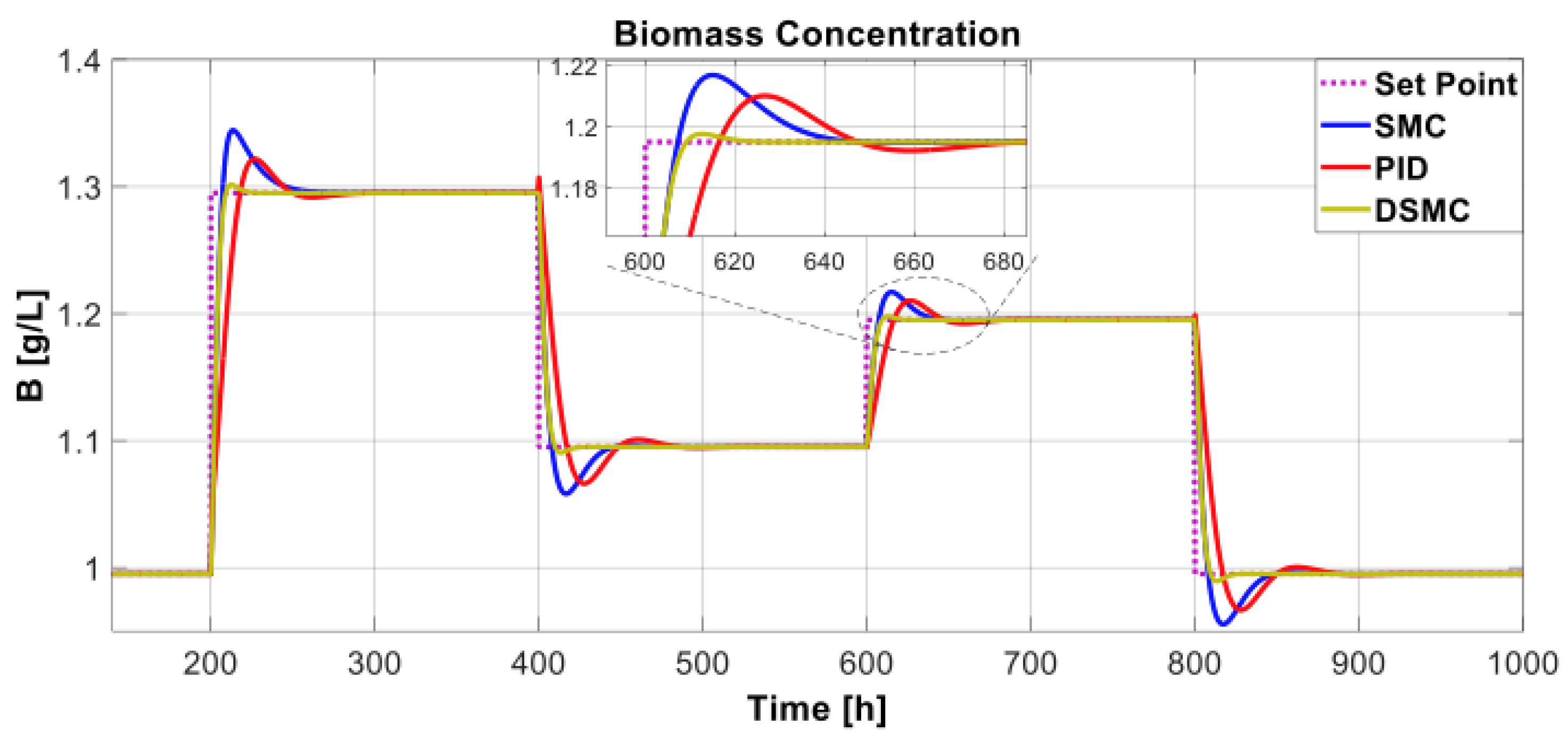
Based on the mentioned concepts, herein, by simulation, we designed and tested a DSMC for unstable open-loop systems with time delay, employing the ideas of sliding modes and internal model structures. The obtained controller has an internal P/PD controller to provide systems with disturbance rejection. In addition, the DSMC corrects modeling errors, providing better performance and increasing the lifetime of the final control element. The proposed DSMC was applied to a nonlinear bioreactor operating at an unstable point [
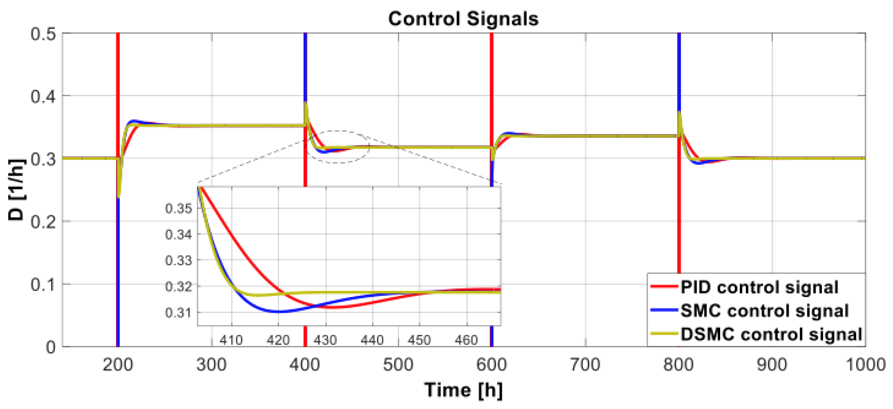
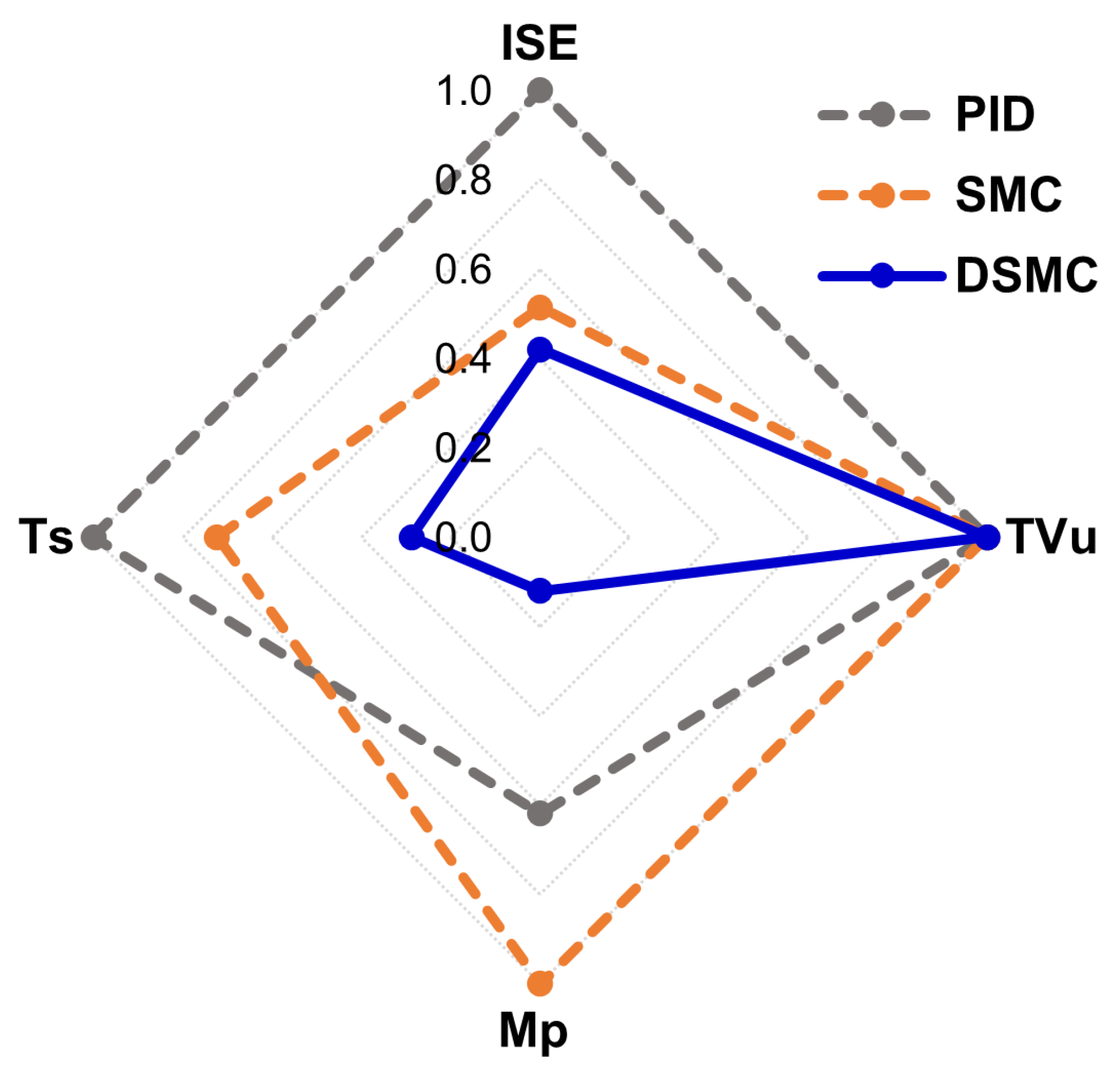
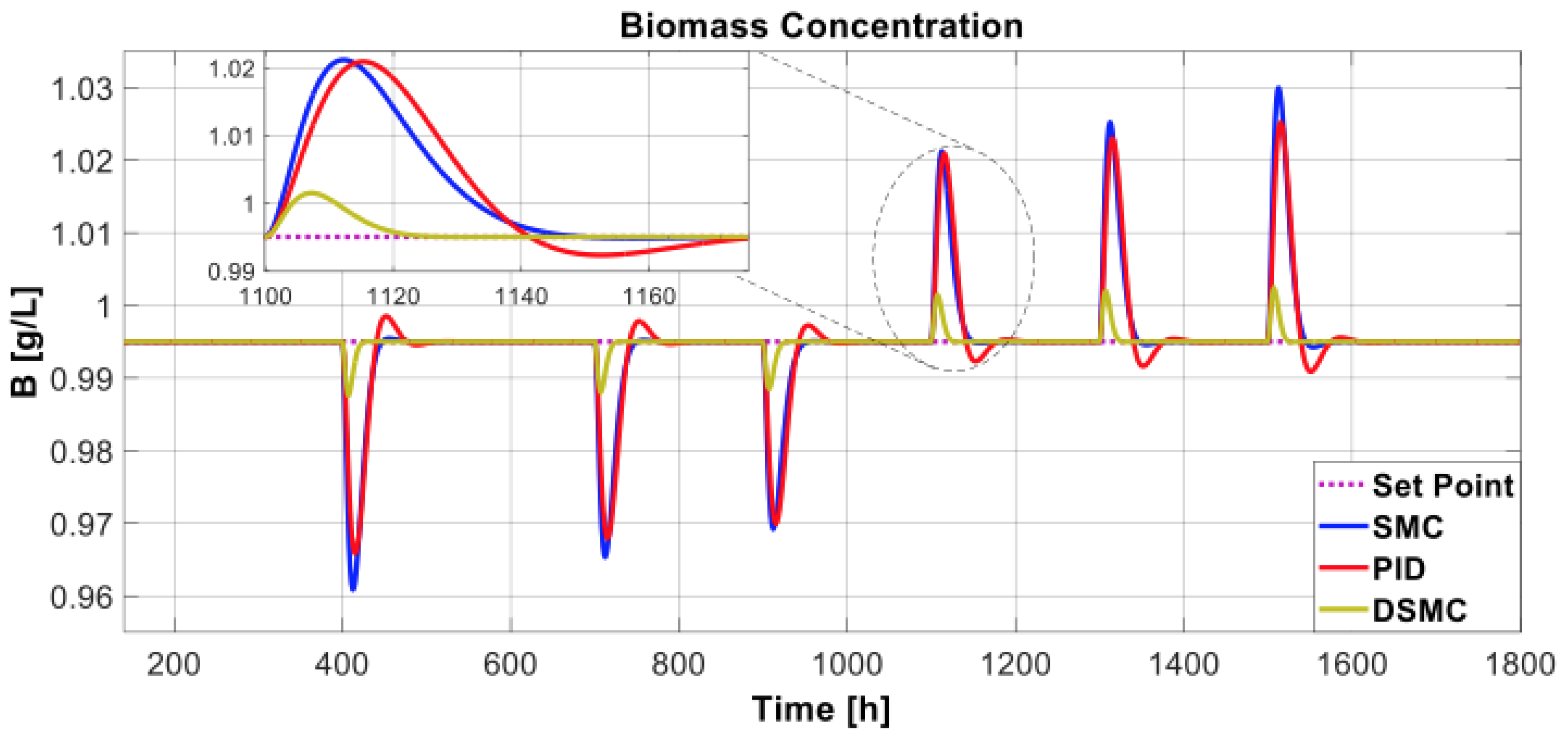
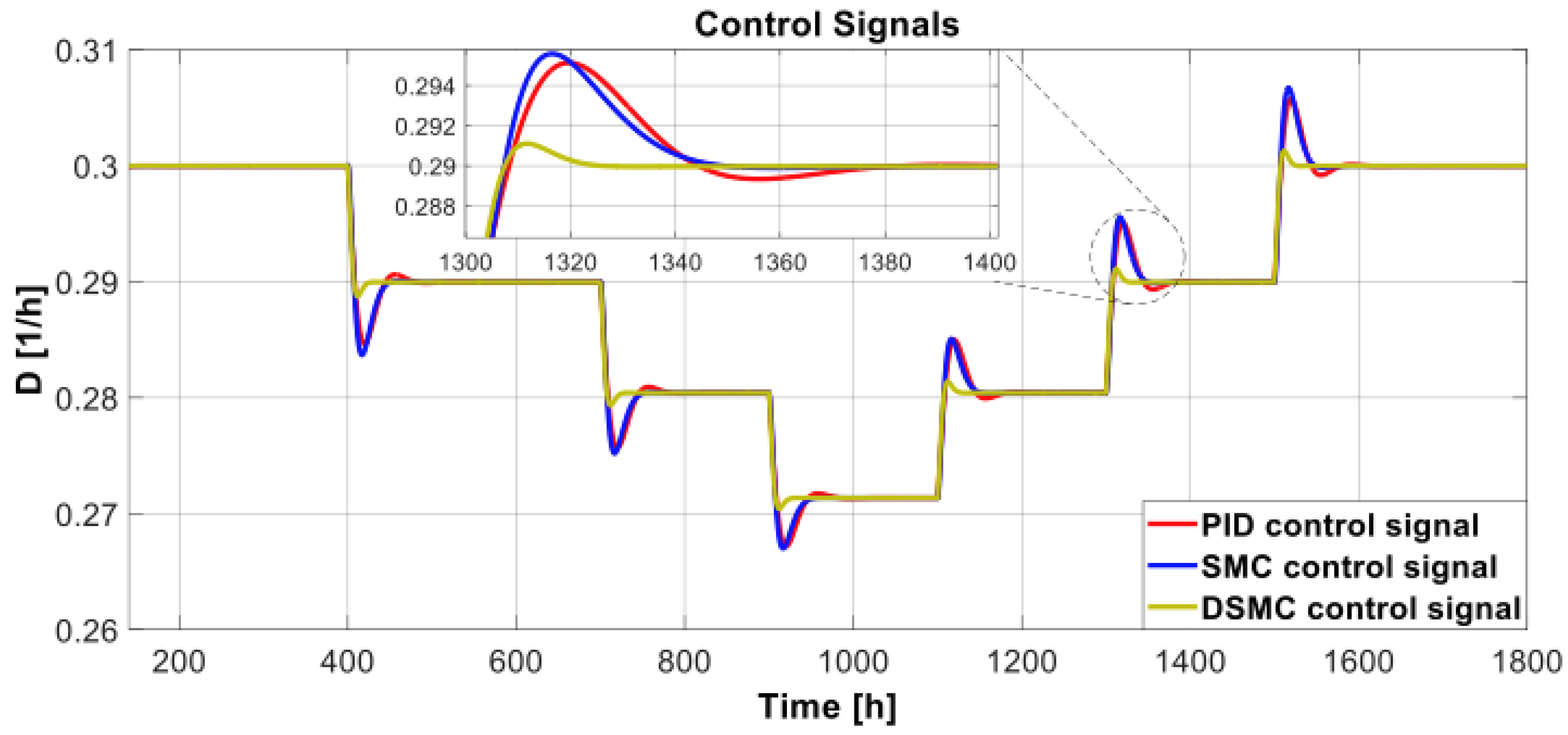
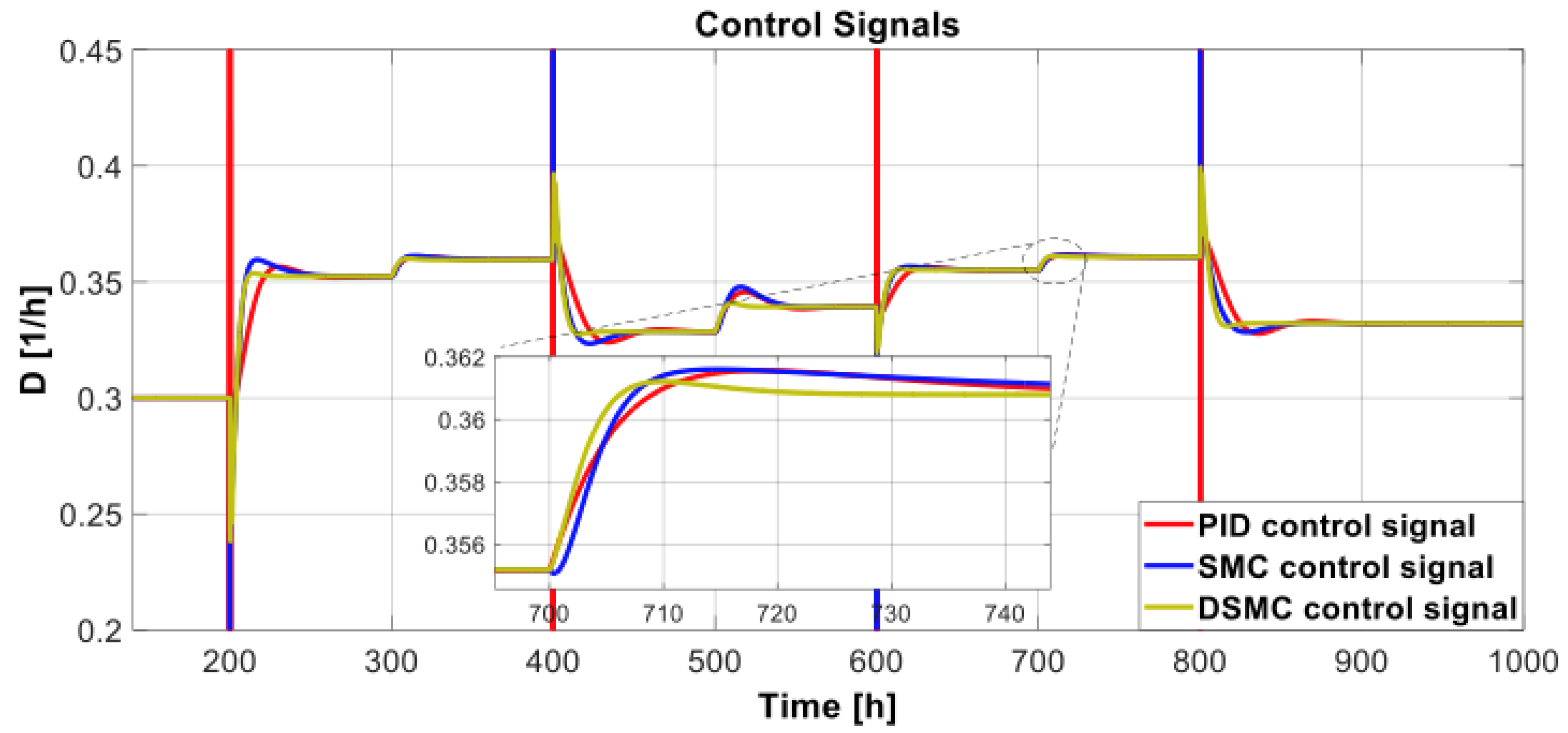
18] and was compared with the SMC presented in [17] and the PID developed in [
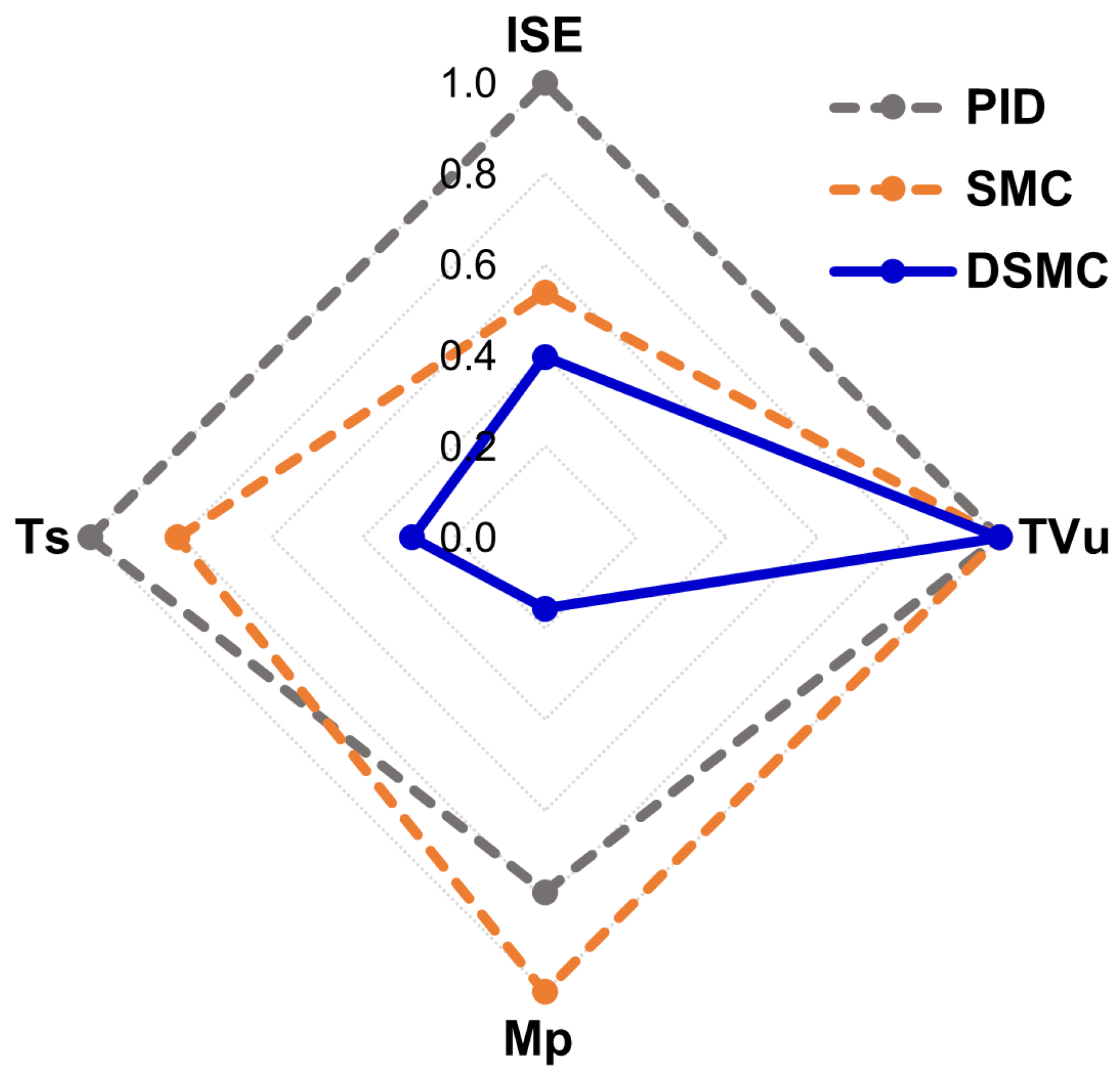
29]. The performance analysis of the control schemes was evaluated based on various indices and transient characteristics, including the integral square error (ISE), the total variation of control effort (TVu), the maximum overshoot (Mp), and the settling time (ts).
The main novelties and contributions of this paper are as follows: (i) a controller for chemical processes with an unstable open-loop response and time delay was designed and implemented by combining the concepts of IMC and SMC; (ii) the controller was developed based on a reduced-order model of the process, specifically the first-order delayed unstable process (FODUP), avoiding a complex model, resulting in a controller of fixed structure easy to implement in any computer system; (iii) the DSMC design approach has a smooth transition, and enhances tracking and disturbance rejection compared with SMC and PID; and (iv) to the best of the authors’ knowledge, this approach has not been previously employed in open-loop unstable nonlinear chemical processes.
The rest of the paper is organized as follows: Section 2 presents, in brief, the basic concepts of unstable systems, IMCs, and SMC; Section 3 presents an unstable system using a PI/PID controller; and Section 4 describes the nonlinear system for testing the controller and discusses their results. Finally, Section 5 presents the conclusions of the study.

2. Background

This section provides a brief overview of several fundamental concepts that underpin our proposed approach’s design, including unstable systems, Internal Model Control, and Sliding Mode Control.

2.1. Unstable Systems

Control engineering is based on the fundamentals of feedback theory and the analysis of nonlinear systems [30]. Feedback control is common in modern technologies, including applications requiring low stationary errors and high performance. In industrial process control applications, stabilizing unstable open-loop plants is critical. Unstable systems have at least one pole on the right-hand side of the complex plane ( j ω ); thus, their behavior cannot be predicted because the output of the systems exhibits sustained growth. Furthermore, unstable processes have inherent control complexity, mainly when a dominant time delay occurs in the system response. Thus, several approaches have been developed to control unstable processes using classical techniques [18,31].

2.2. Internal Model Control

Garcia and Morari proposed IMC in 1982, but several researchers had independently employed a similar concept, following the IMC design procedure. The complexity of the controller depends on the complexity of the model and the performance requirements preset by the designer [32]. IMC employs a systematic procedure for designing control systems based on the Q-parameterization concept, which is the basis of many modern control techniques. Thus, IMC is widely employed in process industries, particularly for tuning single-loop PID controllers [27,32].

2.3. SMC Fundamentals

SMC has been widely employed, owing to the simplicity of its design, reduced complexity of feedback design from reduced-order models, invariance to process dynamic characteristics and external disturbance rejection, good regulation and tracking task performance, and easy implementation in distributed control systems (DCS) [18,27,31]. SMC is a robust control approach that offers a systematic approach to the problem of maintaining stability and consistent performance when modeling uncertainties are present. However, the main disadvantage of this controller is the unwanted vibrations due to the high-frequency switching of the controller, a phenomenon known as chattering [3].
The control principle of SMC is defined in two parts: continuous and discontinuous. The continuous part ensures that the system output is on the desired sliding surface. In contrast, the discontinuous part ensures the system reaches the surface [7]. The feedback control principle is first selected to design the controller to verify the sliding condition. The sliding surface must be discontinuous to compensate for the modeling inaccuracies and disturbances. On the other hand, the discontinuous control principle must be adequately smoothed to achieve the right balance between the control bandwidth and tracking accuracy [3].

3. Identification Procedure for Unstable Systems Using PI/PID Control

This section describes a method for identifying the characteristic parameters of a model for designing the controller using a single experiment on a closed loop system with a step-change in the set-point of the PI or PID controller. This method was first proposed by Yuwana and Seborg [33], extended by Kavdia and Chidambaram [34], and modified by Ananth and Chidambaram [28]. The details of the procedure can be found in [28,34]. It should be noted that open-loop identification methods are not suitable for unstable systems.
In most previous studies, it was assumed that the dynamics of an open-loop unstable process with a positive pole and dead time could be described by a transfer function as follows:
G p ( s ) = K τ s 1 e t 0 s
where K is the gain, τ is the time constant, and t 0 is the dead time.
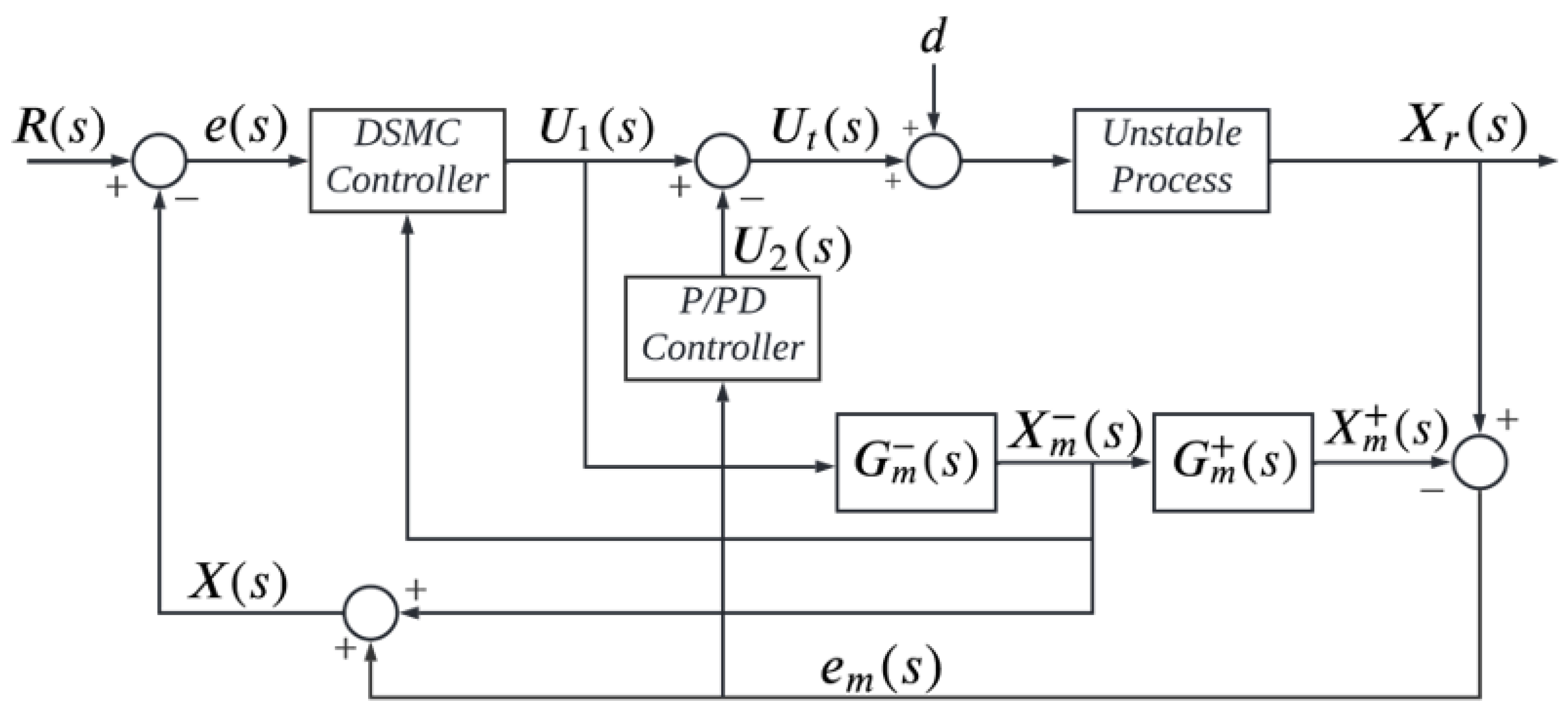
Figure 1 shows the block diagram employed herein, with the required PI/PID controller in a closed-loop [28].
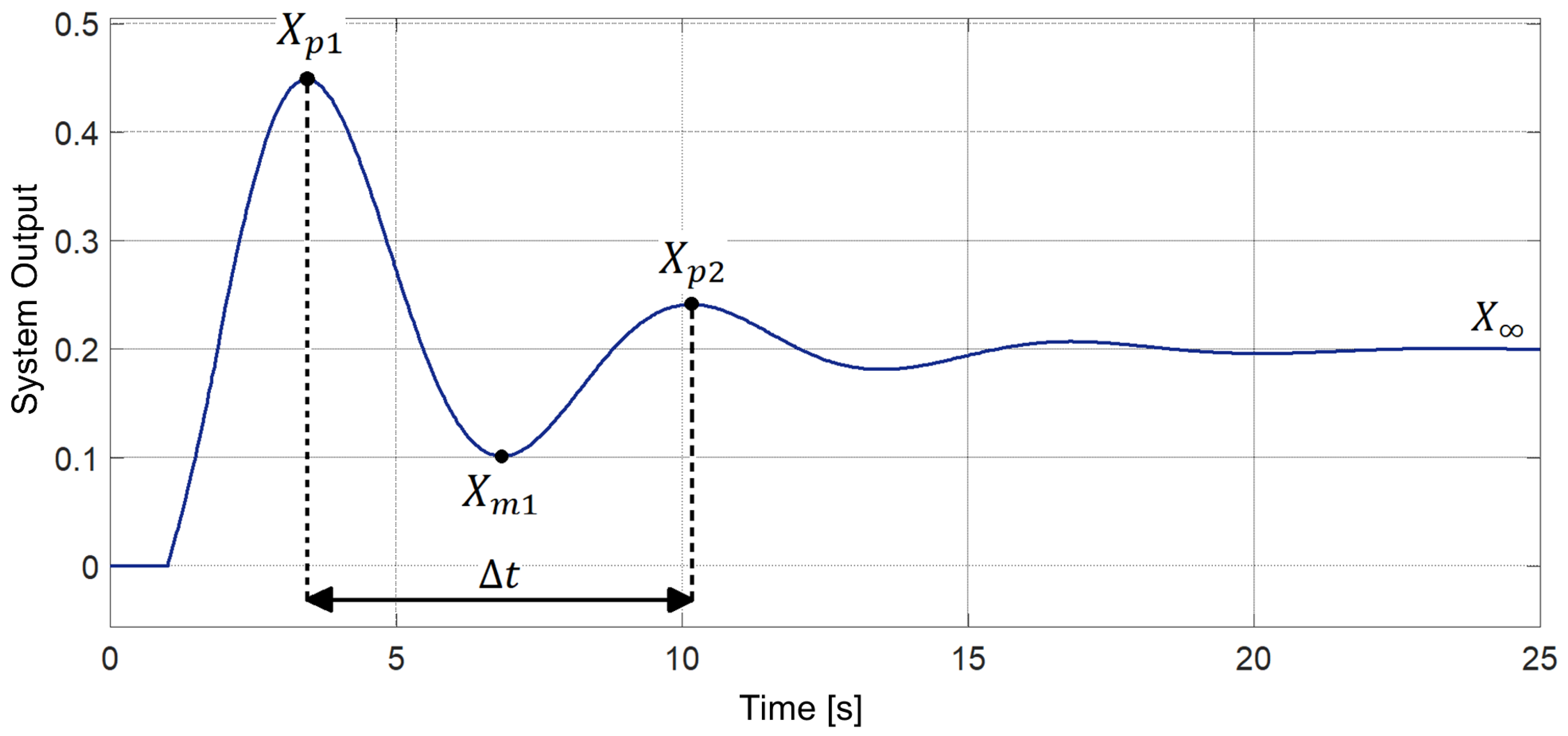
The excitation of the system is a step-input value. The controller constant values are varied until the system response is similar to or equal to that shown in Figure 2.
The response in Figure 2 provides the parameters for determining the FODUP model of the unstable system, which include the following: X p 1 , the first peak of the response; X m 1 , the first minimum value of the response; X p 2 , the second peak of the response; X , the steady-state response value; and Δ t , the time difference between X p 1 and X p 2 . Based on the values of these parameters and the PID constants ( K c , τ i , and τ d ), the first-order model values are determined from the equations proposed in [28], as shown:
K = 2 α 2 β + α 2 β 2 β α 2 β 2 B 2 A α β
τ = α B A β α 2 β 2 B 2 A α β
where:
α = ξ τ e ,
β = ( 1 ξ 2 ) 0.5 τ e ,
ξ 1 = ln ( v 1 ) π 2 + ( ln ( v 1 ) ) 2
ξ 2 = ln ( v 2 ) 4 π 2 + ( ln ( v 2 ) ) 2 ,
ξ = 0.5 ( ξ 1 + ξ 2 ) ,
τ e = Δ t 2 π ( 1 ξ 2 ) 0.5 ,
v 1 = X X m 1 X p 1 X ,
v 2 = X p 2 X X p 1 X
A = K c e t 0 α τ d ( α 2 β 2 ) + α + 1 τ i cos ( t 0 β ) + ( 2 α β τ d + β ) sin ( t 0 β )
B = K c e t 0 α ( 2 α β τ d + β ) cos ( t 0 β ) τ d ( α 2 β 2 ) + α + 1 τ i sin ( t 0 β )
Notably, the time delay t 0 is obtained from the initial part of the response to the step input. Besides, in a case where the controller is a PI, the derivative constant τ d is 0. In summary, the identification method uses the closed-loop response shown in Figure 2 to obtain the first-order open-loop unstable model using the equations proposed in [28].
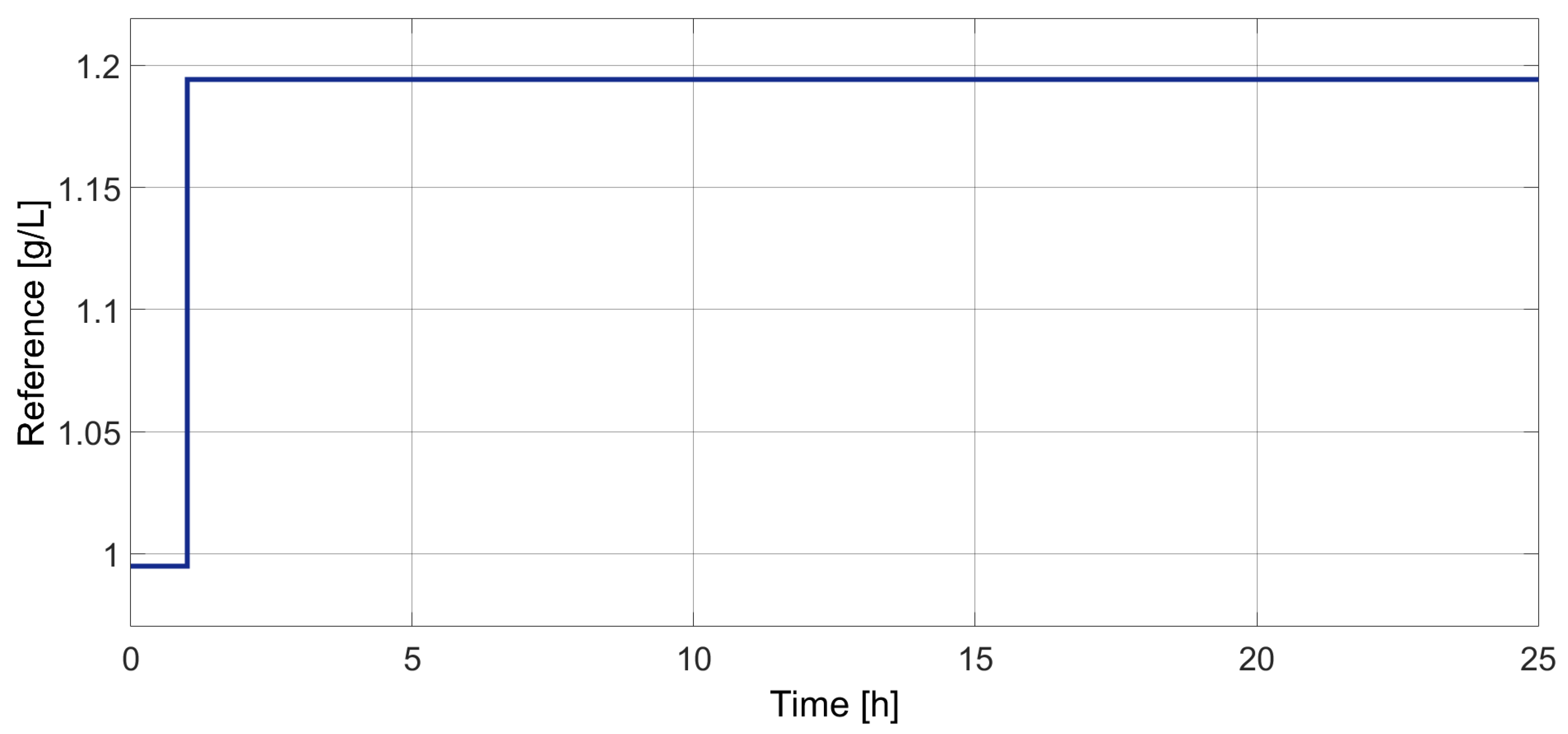
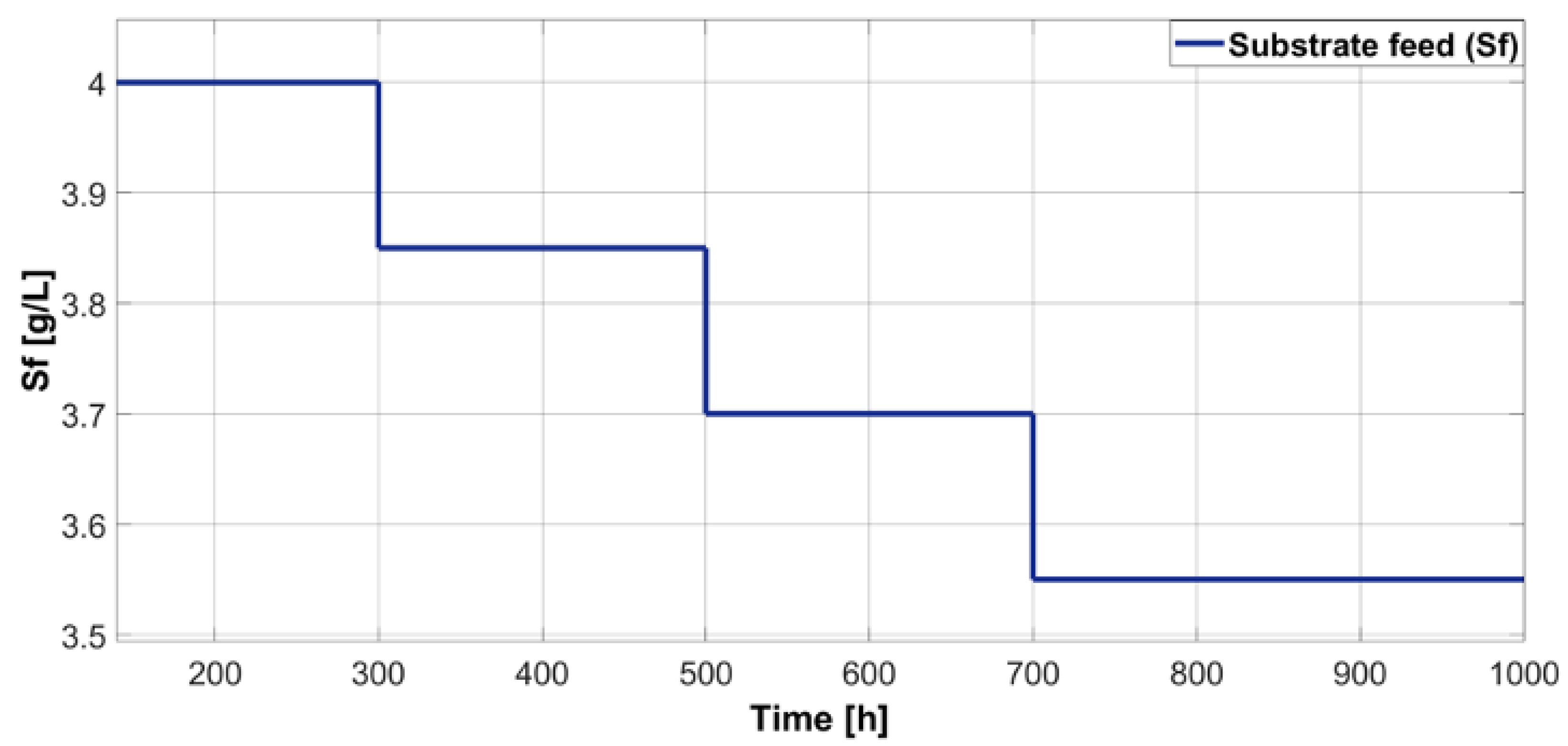
The identification method of the chemical process starts with an input setting that has an initial amplitude of 0.995 [g/L] and then, after 1 [h], grows to 1.194 [g/L] as shown in Figure 3.
PID controller is tuned from the linearized model G L ( s ) . The linearized model is obtained from [28]:
G L ( s ) = 5.89 5.96 s 1 e s
Also, the tuning parameters of the PID controller are acquired from [28], where: K p = 0.7356 , τ i = 4 and τ d = 0.2 . The expression of the PID controller is shown below.
G P I D ( t ) = 0.7356 e ( t ) + 1 4 e ( t ) d ( t ) + 0.2 d e ( t ) d t
With the reference shown in Figure 3 and the PID controller shown in Equation (15), the response of the chemical process is shown in Figure 4.
The identification parameters shown in Table 1 are obtained from the process output shown in Figure 4.
From the identification parameters and the equations proposed in [28], the process can be represented by the transfer function shown in Equation (16).
G p = 6.057 5.959 s 1 e s
Figure 5 shows the response of the process using the PID controller. The nonlinear process and process modeling do not show marked differences, so the identified model is ideal for use in the controller’s design.

4. Dsmc Design Approach

This section describes the design of the proposed approach. Figure 6 shows the proposed scheme. A P or PD controller appears in the inner loop for an adequate response to disturbances. On the other hand, the outer loop consists of the DSMC, which provides robustness and performance against modeling errors and reference changes. Additionally, the scheme has an internal model similar to the Smith predictor to compensate for time delays [13].

4.1. Controller Synthesis

This part presents the design of DSMC for open-loop unstable systems. The DSMC is oriented toward open-loop unstable high-order nonlinear chemical processes that FODUP models can approximate.
The FODUP (Equation (1)) is the basis for the controller synthesis. This equation can include dynamics with poles and zeros defined by a same-time constant τ f as proposed in [12]; re-writing the FOPUD model, it can be represented as follows
G p ( s ) = K t f s + 1 τ s 1 e t o s t f s + 1 .
Notice that the process model in Equation (17) can be separated into an invertible transfer function and in a non-invertible one [32]. The invertible part is G m s and noninvertible part is G m + s of the system:
G m s = X m s U 1 s = K t f s + 1 τ s 1 .
G m + s = e t o s t f s + 1
G m s is taken for the controller design because the inverse of G m + s can be noncausal. So, these noncausal models are not physically possible; this behavior cannot happen [12,32,35].
The performance of the process response depends on the chosen sliding surface. How the SMC works depends on the sliding surface, and changing the sliding surface can change how well the SMC works [3,15,36,37]. The sliding surface selected from [12], shown in Equation (20), is employed:
S ( t ) = K p e ( t ) + λ 0 t e ( t ) d t
Applying the Filippov [3] condition to the previous equation, the above expression is derived and equated to zero to meet the sliding condition,
d S ( t ) d t = K p d e ( t ) d t + λ e t = 0
where e ( t ) and e ( t ) are expressed in Equations (22) and (23), respectively:
e t = R t X m t
e t = R t X ( t )
Based on Equation (22), Equation (24) is obtained.
d e ( t ) d t = d R ( t ) d t d X m t d t
Equation (24) is substituted into Equation (21) to obtain Equation (25):
K p d R t d t d X m t d t + λ e t = 0
From Equation (25), it is obtained in Equation (26):
d X m t d t = d R t d t + λ K p e ( t ) .
Now, to determine the continuous part of the controller, we start from Equation (18), which can be expressed as follows:
τ X m s s X m s = K t f U 1 s s + K U 1 s
Equation (27) in the time domain is given as follows:
τ d X m t d t X m t = K t f d U 1 ( t ) d t + K U 1 ( t )
Equation (26) is substituted into Equation (28) to obtain Equation (29), as follows:
d R t d t + λ K p e t X m t = K t f d U 1 t d t + K U 1 t
From Equation (29), the continuous part of the controller is obtained as follows:
d U C ( t ) d t = τ K t f d R t d t + τ λ K K p t f e t 1 K t f X m t 1 t f U 1 t .
The discontinuous part of the controller is defined by the sign function, as expressed in Equation (31):
d U D t d t = K D s i g n S t .
The K D is an adjustable gain for the discontinuous part of the controller; it was obtained using the Nelder–Mead algorithm [38], as expressed in Equation (32):
K D = 0.51 | K | τ t o 0.76
Equation (20) can be written to ensure proper controller action, as expressed in Equation (33):
S t = s i g n K K p e ( t ) + λ 0 t e ( t ) d t
Note that s i g n   ( K ) is only a sign function of the static gain K to indicate the controller action (direct or reverse); therefore, it does not affect the sliding mode region or change the control switching over U 1 ( t ) .
DSMC is the joint of continuous and discontinuous parts [13], as expressed in Equation (34):
d U 1 t d t = d U C t d t + d U D t d t .
The final DSMC is presented in Equation (35):
d U 1 t d t = τ K t f d R t d t + τ λ K K p t f e t 1 K t f X m t 1 t f U 1 t + K D s i g n S t
Depending on the performance of the controller, d R t d t can be simplified. This does not affect the controller performance; thus, this can be simplified as follows:
d U 1 t d t = τ λ K K p t f e ( t ) 1 K t f X m ( t ) 1 t f U 1 ( t ) + K D s i g n S t
The parameter λ is obtained from [38] and is expressed as follows:
λ = τ + t 0 τ t 0

4.2. Stability Analysis

To analyze the stability of the sliding surface, the Lyapunov criteria have been used in this work [3,38]. If the projection of the system’s trajectories on the sliding surface is stable, then the system is stable.
Theorem 1.
If there exists a candidate Lyapunov function V = 1 2 S ( t ) 2 , which is a positive definite function and its derivative is negative everywhere except for the discontinuity surface, then the following inequality must satisfy the Lyapunov stability condition:
Proof. 
The Lyapunov theorem gives the reaching condition, and the following inequality must be satisfied:
S ( t ) d S ( t ) d t < 0
From Equations (21)–(23), the derivative of the sliding surface is given as follows:
d S ( t ) d t = k p d R t d t d X m t d t + λ e t
Recovering the process model of Equation (28) previously stated, we obtain the following equation:
τ d X m t d t X m t = K t f d U 1 t d t + K U 1 t ,
and substituting Equation (35) into the previous equation, the following result is obtained:
d X m t d t = K τ f τ τ K τ f d R t d t + τ λ K k p τ f e ( τ ) 1 K τ f X m ( τ ) 1 τ f U 1 ( t ) + K D s i g n [ S ( t ) ] + K τ U 1 t + 1 τ X m t .
Equation (41) can be rearranged as follows:
d X m t d t = d R t d t + λ K p e t 1 τ X m t K τ U 1 + K D τ K τ f s i g n S t + K τ U 1 t + 1 τ X m t .
Now, by replacing Equation (35) with Equation (39), the following is obtained:
d S ( t ) d t = K p d R t d t d R t d t 1 K p λ e t K D τ K τ f s i g n ( S ( t ) ) + λ e t
From the previous equation, the following equation is obtained:
d S ( t ) d t = K D K p τ K τ f s i g n S t
Let K D = K D K p τ K τ f ; then:
S ( t ) d S ( t ) d t = K D | S ( t ) | < 0 i f K D > 0
Thus,
K D | S ( t ) | < 0
Finally, to guarantee the stability of the controller, K D > 0

4.3. Internal P/PD Controller Design

The internal P/PD controller helps the system respond adequately to disturbance changes. The proportional tuning value is based on the optimal phase margin [39], as expressed in Equation (47):
P s = K c = 1 ϵ 0 < ϵ < 1
The expression of the PD controller is expressed in Equation (48) [31]:
P D s = K c 1 + τ d s 0.1 τ d s + 1 .
The expressions to determine the values of the PD controller constants are as follows [31]:
K c = 1 K 0.820 t 0 τ 0.817 + 0.278
τ d = τ 0.008 t 0 τ 2 + 0.467 t 0 τ + 0.006

5. Computer Simulations

This section first presents the non-linear mathematical model of the biochemical process chosen to test the performance of the proposed DSMC. Then, several indices are used to evaluate the performance of the controllers. The proposed DSMC, SMC [38], and PID [29] are applied to the non-linear process; likewise, they are tested and compared. The parameters used in simulation for the mentioned controllers are shown in Table 2.

5.1. Biochemical Reactor Model

A biochemical reactor that operates at an unstable point is considered to perform regulatory and tracking tests. A detailed description of the process with mathematical modeling and parameter values is given in Galluzzo [18], originally presented by Agrawal and Lim [40]. It should be noted that operation at unstable points is a frequent practice in chemical and biochemical processes. This condition allows operation at a maximum gradient for mass transfer and chemical reaction, which gives a faster process. To apply the control proposed here, two parts are presented. First, the identification method is applied to the nonlinear process, and the characteristic parameters ( K , τ , and t 0 ) are obtained and used in the controller equation. After that, the controllers are applied to the mentioned nonlinear process. Then, three control schemes (SMC, PID, and DSMC) are tested and compared. Finally, the process output and the control action for all controllers are compared using the nonlinear process as the real plant. Additionally, radial graphs showing performance indices and transient criteria, including maximum overshoots and settling times, are used to evaluate the performance of various controllers.
The bioreactor (Figure 7) is an unstable nonlinear system. The graph shows the elements that make up the system to be controlled. Given the conditions of the process, it works at the unstable equilibrium point despite the lower conversion because, at the stable equilibrium point, there is biomass inhibition, causing oscillations in the states and reducing productivity. In this bioprocess, the control objective is to drive the biomass concentration ( B ( t ) ) from the stable equilibrium point (higher conversion) to the unstable equilibrium point (lower conversion), despite the perturbations and uncertainties of the model. The dilution rate D is the manipulated variable, while the feed substrate is the main disturbance of the process, and B ( t ) is the process output.
The following differential equations describe the biomass and substrate concentration:
d B ( t ) d t = μ D t B ( t )
d S ( t ) d t = D S f S ( t ) μ B ( t ) γ
μ = μ m a x S ( t ) k m + S ( t ) + k 1 S ( t ) 2
where:
B ( t ) : Biomass concentration
S ( t ) : Substrate concentration
D ( t ) : Dilution rate
S f : Substrate concentration on process feeding (main process disturbance)
μ : Specific growth rate
μ m a x : Maximum specific growth rate
k m : Substrate saturation constant
k 1 : Substrate inhibition constant
γ : Biomass to substrate mass yield
The parameters and initial conditions of the process are shown in Table 3, where each variable is represented by its respective units.
From the procedure described by Ananth and Chidambaram [28], the nonlinear process can be approximated to a FODUP model (Equation (1)). The FODUP model was expressed in Equation (16). Once K , τ , and t 0 are known, K D and λ can be calculated using Equations (32) and (37), respectively. Meanwhile, K p and t f are determined by trial and error until the controller provides an adequate response. On the other hand, the values of the internal PD constants ( K c and τ d ) are calculated using Equations (49) and (50).

5.2. Control Performance Indices

There are many ways to evaluate the performance of process controllers. However, most of them involve comparing the quality of control with some standard or desired value [35,41,42,43]. In this part, the integral of squared error (ISE), the integral of the total variation of the control signal (TVu), the maximum overshoot, and the settling time (Ts) are considered performance indices to evaluate the proposed approach against the PID and the SMC controllers.
Integral of the Squared Error (ISE): It is a measure of the performance of the system calculated by integrating the square of the error of the system over a fixed period. It places more weight on large errors, which usually occur at the beginning of the response, and less on smaller errors, which occur toward the end. A small value of this quantity indicates small variations of the processed signal concerning the setpoint, increasing the efficacy of the process [35,43,44].
I S E = 0 e ( t ) 2 d t
Integral of the total variation of the control signal (TVu): It is an indicator of the effort of the control signal. It can be determined according to the following expression:
T V u = k = 1 u k + 1 u k
where u k and u k + 1 are the current and next-step values of the control signal, respectively. A small value of this quantity indicates smooth variations of the control signal, increasing the useful life of the final control element [42].
Peak Overshoot (Mp): It is defined as the deviation of the response at the time where a maximum peak appears, regarding the final or desired value of the response. It, also called the maximum overshoot, is the amount of the output system that exceeds its target value in %. The percentage of overshoot is the maximum value minus the steady-state value divided by the steady-state value and the result multiplied by 100 [35].
Settling time (Ts): Is the time required for the response to reach a steady state and remain within the specified tolerance bands around the final value. The normally used tolerance bands are 2 % and 5 % [35].

5.3. Tracking Performance Test

A tracking test was performed by varying the biomass concentration every 200 h. It started with an initial state of 0.995 g/L. Then, at 200 h, the biomass increased to 1.295 g/L, and at 400 h, it decreased to 1.095 g/L, after which the biomass grew again at 600 h, and the tracking reached 1.195 g/L. Finally, the biomass reached 800 h, and the tracking returned to 0.995 g/L. Figure 8 shows the behavior of the system and the controllers implemented. The proposed DSMC had a slight overshoot, presenting a faster response and greater robustness based on SMC and PID. This faster response reduces the settling time to 20 h, half or less than the other controllers.
The three simulated control signals were similar. However, the DSMC showed a slightly higher peak in the transient-state response than the others. However, DSMC showed a faster signal than PID and SMC, again only 20 h compared with 40 or more for the other controllers. However, the PID and SMC control signals showed significant peaks when the amplitude of the set-point changed (Figure 9).
Table 4 and Figure 10 show the performance indices and transient parameters for changes in the set-point of the biochemical reactor. DSMC shows the lowest ISE, indicating that DSMC exhibits the best performance. The Tvu performance index for the three controllers remained the same. On the other hand, DSMC showed the lowest value of the maximum transient overshoot, reflected in the response of the process (Figure 8). DSMC showed a settling time of 26.78 h, less than that of the other controllers (67.28 h and 93.03 h for SMC and PID, respectively).

5.4. Regulation Performance Test

The regulation performance test presented a variation in the disturbance and a constant set-point. The set-point had a constant value of 0.995 [g/L] of biomass, while the disturbance changed its value, as shown in Figure 11. The changes in S f concentration are the main process disturbance. Other changes to process inputs were tested, but the results showed low sensibility regarding process output. Therefore, it was the chosen disturbance. The variation in substrate feed concentration altered the dynamics of the biochemical reactor.
The graph in Figure 12 shows the performance of the biochemical reactor subjected to variations in substrate feed ( S f ) variations. Again, DSMC presented greater robustness since the response presented minimum peaks for the other controllers. Furthermore, in Figure 13, DSMC showed a smoother signal in response to variations S f and had a lower peak than SMC and PID.
Table 5 and Figure 14 show the performance indices of the substrate feed variations and the transient parameters. DSMC presents greater robustness and performance than other controllers because it has smaller ISE, Mp, and Ts. The TVu performance index is almost the same for all three controllers. However, in Figure 13, DSMC presents a lower peak when the substrate feed changes the amplitude. DSMC achieved the correct response trajectory in disturbance rejection faster than other controllers.

5.5. Regulation and Tracking Performance Tests

In the regulation and tracking performance tests, we used the same set point changes used in the tracking test and substrate feed variation shown in Figure 15. The perturbation started with the nominal value of 4 [g/L]; at 300 [h], it decreased to 3.85 [g/L]; at 500 [h], it further decreased to 3.7 [g/L]; finally, with the substrate feed at 700 [h], it decreased to 3.55 [g/L]. Figure 15 shows the changes in the feed substrate.
Figure 16 shows the performance of the biochemical reactor when set-point and perturbation changes occur. Although the system performance for set-point changes has already been analyzed, the disturbance ( S f ) changes the system performance. In this case, the DSMC showed a faster signal than the others and quickly reached the set point. On the other hand, SMC and PID had higher overshoots than DSMC. Therefore, we conclude that the proposed DSMC is the most robust controller. Furthermore, the control signals for the three controllers were similar (Figure 17), considering that when the magnitude of the set-point changed, the PID controller showed high peaks.
Table 6 and Figure 18 show the performance indices and transient parameters of the biochemical reactor as the substrate feed and the set point vary. DSMC performed better than SMC and PID because DSMC had the smallest ISE. Furthermore, DSMC showed the lowest overshoot, with a value of only 0.343%, approximately 2.198%, and 1.714% for SMC and PID, respectively. On the other hand, the three controllers showed the same TVu. Finally, the settlement time of the DSMC was 26.96 h, which is approximately three and three and a half times less than that of the SMC and the PID, respectively.

6. Conclusions

In this study, a DSMC was developed that combines the concepts of the internal model and sliding mode control. The controller synthesis used a FODUP model of actual processes. The DSMC aims to reduce chattering effects in the control signal. Additionally, an internal loop with a PD controller was incorporated to provide the system with a suitable response to disturbances. The computer simulation of the proposed controller in a bioreactor revealed that the performance of the controller is stable and satisfactory despite nonlinearities in the operating conditions, set-point changes, process disturbances, and modeling errors.
Furthermore, DSMC improved tracking and regulatory tasks by reducing half or more of the response time compared with PID and SMC controllers. Thus, the internal PID controller provides a better response to disturbances. Furthermore, DSMC remarkably balances the response speed and smoothness of the control action. Therefore, considering the incidence of the final control elements, a quick and smooth control response is attained.
Future work for this research includes the use of optimization algorithms to find appropriate parameters or tuning equations for the proposed controller.
In addition, to further validate the proposed control strategy in real-time, Hardware In the Loop (HIL) simulations can be used to implement the proposed algorithm in an embedded system and simulate the dynamics of a nonlinear, unstable chemical process using Matlab®.

Author Contributions

Conceptualization, C.C. and O.C.; methodology, C.C., J.E. and O.C.; software, C.C., J.E.; validation, C.C., H.A., J.E. and O.C.; formal analysis, C.C., H.A., J.E. and O.C.; investigation, C.C. and O.C.; resources, O.C.; data curation, C.C. and J.E.; writing—original draft preparation, C.C., H.A, J.E. and O.C; writing—review and editing, C.C., H.A., J.E. and O.C.; visualization, C.C. and J.E; supervision, O.C.; project administration, O.C.; funding acquisition, O.C. All authors have read and agree to the published version of the manuscript.

Funding

This research was supported by the Colegio de Ciencias e Ingenieras, Universidad San Francisco de Quito USFQ, through the Poli-Grants Program under Grant 17965.

Acknowledgments

The authors thank the USFQ Advanced Control Systems Research Group, Quito, Ecuador.

Conflicts of Interest

The authors declare no conflict of interest.

References

  1. Huang, H.P.; Chen, C.C. Control-system synthesis for open-loop unstable process with time delay. IEEE Proc. Control Theory Appl. 1997, 144, 334–346. [Google Scholar] [CrossRef] [Green Version]
  2. Sardella, M.F.; Serrano, M.E.; Camacho, O.; Scaglia, G.J. Design and application of a linear algebra based controller from a reduced-order model for regulation and tracking of chemical processes under uncertainties. Ind. Eng. Chem. Res. 2019, 58, 15222–15231. [Google Scholar] [CrossRef]
  3. Utkin, V.; Poznyak, A.; Orlov, Y.V.; Polyakov, A. Road Map for Sliding Mode Control Design; Springer: Berlin/Heidelberg, Germany, 2020. [Google Scholar]
  4. Sira-Ramírez, H. Dynamical sliding mode control strategies in the regulation of nonlinear chemical processes. Int. J. Control 1992, 56, 1–21. [Google Scholar] [CrossRef]
  5. Utkin, V.; Lee, H. Chattering problem in sliding mode control systems. In Proceedings of the International Workshop on Variable Structure Systems, VSS’06, Alghero, Italy, 5–7 June 2006; pp. 346–350. [Google Scholar]
  6. Cortes, D.; Vázquez, N.; Alvarez-Gallegos, J. Dynamical sliding-mode control of the boost inverter. IEEE Trans. Ind. Electron. 2008, 56, 3467–3476. [Google Scholar] [CrossRef]
  7. Koshkouei, A.J.; Burnham, K.J.; Zinober, A.S. Dynamic sliding mode control design. IEEE Proc. Control Theory Appl. 2005, 152, 392–396. [Google Scholar] [CrossRef] [Green Version]
  8. Shtessel, Y.; Edwards, C.; Fridman, L.; Levant, A. Sliding Mode Control and Observation; Springer: Berlin/Heidelberg, Germany, 2014; Volume 10. [Google Scholar]
  9. Liu, J.; Wang, X.; Liu, J.; Wang, X. Advanced Sliding Mode Control; Springer: Berlin/Heidelberg, Germany, 2011. [Google Scholar]
  10. Yu, X.; Feng, Y.; Man, Z. Terminal sliding mode control–an overview. IEEE Open J. Ind. Electron. Soc. 2020, 2, 36–52. [Google Scholar] [CrossRef]
  11. Li, C.; Kim, J.; Lee, M.C. Fast Terminal SMC with SPO for Trajectory Tracking of Robot Manipulator for Nuclear Reactor Dismantlement. In Proceedings of the 2022 22nd International Conference on Control, Automation and Systems (ICCAS), Busan, Republic of Korea, 27 November–1 December 2022; pp. 196–199. [Google Scholar]
  12. Báez, E.; Bravo, Y.; Leica, P.; Chávez, D.; Camacho, O. Dynamical sliding mode control for nonlinear systems with variable delay. In Proceedings of the 2017 IEEE 3rd Colombian Conference on Automatic Control (CCAC), Cartagena, Colombia, 18–20 October 2017; pp. 1–6. [Google Scholar]
  13. Herrera, M.; Camacho, O.; Leiva, H.; Smith, C. An approach of dynamic sliding mode control for chemical processes. J. Process Control 2020, 85, 112–120. [Google Scholar] [CrossRef]
  14. Proaño, P.; Capito, L.; Rosales, A.; Camacho, O. A dynamical sliding mode control approach for long deadtime systems. In Proceedings of the 2017 4th International Conference on Control, Decision and Information Technologies (CoDIT), Barcelona, Spain, 5–7 April 2017; pp. 0108–0113. [Google Scholar]
  15. Coronel, W.; Camacho, O. A Dynamic Sliding Mode Controller using a Rotating Type Moving Sliding Surface for Chemical Processes with Variable Delay. In Proceedings of the 2021 IEEE CHILEAN Conference on Electrical, Electronics Engineering, Information and Communication Technologies (CHILECON), Online, 6–9 December 2021; pp. 1–6. [Google Scholar]
  16. Asimbaya, E.; Cabrera, H.; Camacho, O.; Chávez, D.; Leica, P. A dynamical discontinuous control approach for inverse response chemical processes. In Proceedings of the 2017 IEEE 3rd Colombian Conference on Automatic Control (CCAC), Cartagena, Colombia, 18–20 October 2017; pp. 1–6. [Google Scholar]
  17. Rojas, R.; Camacho, O.; González, L. A sliding mode control proposal for open-loop unstable processes. ISA Trans. 2004, 43, 243–255. [Google Scholar] [CrossRef]
  18. Galluzzo, M.; Cirino, C. Sliding mode fuzzy logic control of an unstable bioreactor. Chem. Eng. Trans. 2013, 32, 1213–1218. [Google Scholar]
  19. Mehta, U.; Rojas, R. Smith predictor based sliding mode control for a class of unstable processes. Trans. Inst. Meas. Control 2017, 39, 706–714. [Google Scholar] [CrossRef] [Green Version]
  20. Pandey, S.; Dourla, V.; Dwivedi, P.; Junghare, A. Introduction and realization of four fractional-order sliding mode controllers for nonlinear open-loop unstable system: A magnetic levitation study case. Nonlinear Dyn. 2019, 98, 601–621. [Google Scholar] [CrossRef]
  21. Siddiqui, M.A.; Anwar, M.N.; Laskar, S.H. Sliding mode controller design for second-order unstable processes with dead-time. J. Electr. Eng. 2020, 71, 237–245. [Google Scholar] [CrossRef]
  22. Kumar, S.; Ajmeri, M. Optimal variable structure control with sliding modes for unstable processes. J. Cent. South Univ. 2021, 28, 3147–3158. [Google Scholar] [CrossRef]
  23. Kumar, S.; Ajmeri, M. Smith predictor–based sliding mode control with hyperbolic tangent function for unstable processes. Trans. Inst. Meas. Control 2023, 01423312221146338. [Google Scholar] [CrossRef]
  24. Espín, J.; Castrillon, F.; Leiva, H.; Camacho, O. A modified Smith predictor based–Sliding mode control approach for integrating processes with dead time. Alex. Eng. J. 2022, 61, 10119–10137. [Google Scholar] [CrossRef]
  25. Camacho, C.; Camacho, O. A Dynamic Sliding Mode Controller Approach for Open-Loop Unstable Systems. In Proceedings of the 2022 IEEE International Autumn Meeting on Power, Electronics and Computing (ROPEC), Ixtapa, Mexico, 9–11 November 2022; Volume 6, pp. 1–6. [Google Scholar]
  26. Sree, R.P.; Chidambaram, M. Identification and Controller Design for Unstable System in Control of Unstable Systems; Alpha Science Int’l Ltd.: London, UK, 2006. [Google Scholar]
  27. Vozäk, D.; Ilka, A. Application of Unstable System in Education of Modern Control Methods. IFAC Proc. Vol. 2013, 46, 114–119. [Google Scholar] [CrossRef]
  28. Ananth, I.; Chidambaram, M. Closed-loop identification of transfer function model for unstable systems. J. Frankl. Inst. 1999, 336, 1055–1061. [Google Scholar] [CrossRef]
  29. Seer, Q.H.; Nandong, J. Stabilization and PID tuning algorithms for second-order unstable processes with time-delays. ISA Trans. 2017, 67, 233–245. [Google Scholar] [CrossRef]
  30. Saat, M.S.M.; Nguang, S.K.; Nasiri, A. Analysis and Synthesis of Polynomial Discrete-Time Systems: An SOS Approach; Butterworth-Heinemann: Oxford, UK, 2017. [Google Scholar]
  31. Irshad, M.; Ali, A. Robust PI-PD controller design for integrating and unstable processes. IFAC-PapersOnLine 2020, 53, 135–140. [Google Scholar] [CrossRef]
  32. Rivera, D.E.; Morari, M.; Skogestad, S. Internal model control: PID controller design. Ind. Eng. Chem. Process Des. Dev. 1986, 25, 252–265. [Google Scholar] [CrossRef]
  33. Yuwana, M.; Seborg, D.E. A new method for on-line controller tuning. AIChE J. 1982, 28, 434–440. [Google Scholar] [CrossRef]
  34. Kavdia, M.; Chidambaram, M. On-line controller tuning for unstable systems. Comput. Chem. Eng. 1996, 20, 301–305. [Google Scholar] [CrossRef]
  35. Marlin, T.E. Process Control: Designing Processes and Control Systems for Dynamic Performance; McGraw-Hill Science, Engineering & Mathematics: New York, NY, USA, 2000. [Google Scholar]
  36. Vásquez, M.; Yanascual, J.; Herrera, M.; Prado, A.; Camacho, O. A hybrid sliding mode control based on a nonlinear PID surface for nonlinear chemical processes. Eng. Sci. Technol. Int. J. 2023, 40, 101361. [Google Scholar] [CrossRef]
  37. Obando, C.; Rojas, R.; Ulloa, F.; Camacho, O. Dual-Mode Based Sliding Mode Control Approach for Nonlinear Chemical Processes. ACS Omega 2023, 8, 9511–9525. [Google Scholar] [CrossRef]
  38. Camacho, O.; Smith, C.A. Sliding mode control: An approach to regulate nonlinear chemical processes. ISA Trans. 2000, 39, 205–218. [Google Scholar] [CrossRef] [PubMed]
  39. De Paor, A.M.; O’Malley, M. Controllers of Ziegler-Nichols type for unstable process with time delay. Int. J. Control 1989, 49, 1273–1284. [Google Scholar] [CrossRef]
  40. Agrawal, P.; Lim, H.C. Analyses of various control schemes for continuous bioreactors. In Bioprocess Parameter Control; Springer: Berlin/Heidelberg, Germany, 1984; pp. 61–90. [Google Scholar]
  41. Moliner, R.; Tanda, R. Herramienta para la sintonía robusta de controladores PI/PID de dos grados de libertad. Rev. Iberoam. Autom. Inform. Ind. 2016, 13, 22–31. [Google Scholar] [CrossRef] [Green Version]
  42. Torralba-Morales, L.; Reynoso-Meza, G.; Carrillo-Ahumada, J. Sintonización y comparación de conceptos de diseño aplicando la optimalidad de Pareto. Un caso de estudio del biorreactor de Cholette. Rev. Iberoam. Autom. Inform. Ind. 2020, 17, 190–201. [Google Scholar] [CrossRef]
  43. Liptak, B.G. Process control and optimization. In Instrument Engineers’ Handbook; CRC Press: Boca Raton, FL, USA, 2018; Volume 2. [Google Scholar]
  44. Smith, C.A.; Corripio, A.B. Principles and Practices of Automatic Process Control; John Wiley & Sons: Hoboken, NJ, USA, 2005. [Google Scholar]
Figure 1. Identification scheme method.
Chemengineering 07 00053 g001
Figure 2. Expected system response to obtain the identification parameters of an unstable system.
Chemengineering 07 00053 g002
Figure 3. Reference for identification method.
Chemengineering 07 00053 g003
Figure 4. Biochemical reactor output for the identification method.
Chemengineering 07 00053 g004
Figure 5. Closed-loop response of the nonlinear model and identified model using the PID controller.
Chemengineering 07 00053 g005
Figure 6. Proposed control scheme. where: R ( s ) : Reference; U 1 ( s ) : DSMC output; U 2 ( s ) : P/PD controller output; U t ( s ) : Total controller output; X m ( s ) : Invertible part output; X m + ( s ) : Non-invertible part output; X r ( s ) : Process output; e ( s ) : Overall error; e m ( s ) : Modeling error; X ( s ) : Total output of the new system.
Chemengineering 07 00053 g006
Figure 7. Biochemical Reactor Process Diagram.
Chemengineering 07 00053 g007
Figure 8. Biochemical reactor output for the set-point changes.
Chemengineering 07 00053 g008
Figure 9. Control signals with changes in the set-point.
Chemengineering 07 00053 g009
Figure 10. Radial graph of the performance indices and transient parameters for the set-point changes.
Chemengineering 07 00053 g010
Figure 11. Perturbation applied to the substrate feed, S f .
Chemengineering 07 00053 g011
Figure 12. Biochemical reactor output for the substrate feed variation.
Chemengineering 07 00053 g012
Figure 13. Control signals for the substrate feed variation.
Chemengineering 07 00053 g013
Figure 14. Radial graph of performance indices and transient parameters for substrate feed variations.
Chemengineering 07 00053 g014
Figure 15. Perturbation applied to the substrate feed, S f .
Chemengineering 07 00053 g015
Figure 16. Biochemical reactor output with substrate feed variations and set-point changes.
Chemengineering 07 00053 g016
Figure 17. Control signals with substrate feed variations and set-point changes.
Chemengineering 07 00053 g017
Figure 18. Radial graph of performance indices and transient parameters with substrate feed variations and set-point changes.
Chemengineering 07 00053 g018
Table 1. Identification parameters.
ParameterNominal Value
X p 1 1.391 [g/L]
X m 1 1.143 [g/L]
X p 2 1.208 [g/L]
X 1.194 [g/L]
Δ t 9.200 [h]
k p −0.740
τ i 3.300
τ d 0.200
Table 2. Controller tuning parameters for biochemical reactor.
Controllers
ParameterDSMCSMCPID
K−6.057−6.057-
τ 5.9595.959-
t 0 11-
t f 4--
k p 0.200--
l d 5.200--
l d 0 -0.062-
l d 1 -0.500-
K c −0.637-−0.347
τ i --20.12
τ d 0.502-1.666
ϵ --4.5
Table 3. Operation conditions of the biochemical reactor.
ParameterNominal ValueParameterNominal Value
γ 0.40 [g/g] k 1 0.455 [g/L]
S f 4.00 [g/L]D0.300 [h 1 ]
μ m a x 0.53 [L/h] B ( 0 ) 0.995 [g/L]
k m 0.12 [g/L] S ( 0 ) 1.512 [g/L]
Table 4. Performance indices and transient parameters with changes in the set-point.
ControllerIndices
ISETVuMp [%]Ts [h]
DSMC0.339279.10.36026.78
SMC0.415279.23.00167.28
PID0.807279.21.85893.03
Table 5. Performance indices and transient parameters for the substrate feed variations.
ControllerIndices
ISETVuMp[%]Ts [h]
DSMC0.0023479.40.67025.75
SMC0.0773479.83.19677.39
PID0.0834479.82.814110.06
Table 6. Performance indices and transient parameters with substrate feed variations and set-point changes.
ControllerIndices
ISETVuMp [%]Ts [h]
DSMC0.347294.00.34326.96
SMC0.470294.22.19874.70
PID0.873294.21.71492.56
Disclaimer/Publisher’s Note: The statements, opinions and data contained in all publications are solely those of the individual author(s) and contributor(s) and not of MDPI and/or the editor(s). MDPI and/or the editor(s) disclaim responsibility for any injury to people or property resulting from any ideas, methods, instructions or products referred to in the content.

