Article

Identification of Unknown Substances in Ambient Air (PM10), Profiles and Differences between Rural, Urban and Industrial Areas

1
Foundation for the Promotion of Health and Biomedical Research in the Valencian Region, FISABIO-Public Health, 21, Avenida Catalunya, 46020 Valencia, Spain
2
Environmental and Public Health Analytical Chemistry, Research Institute for Pesticides and Water, University Jaume I, S/N, Avenida Sos Baynat, 12071 Castelló de la Plana, Spain
3
Public Health Laboratory of Valencia, 21, Avenida Catalunya, 46020 Valencia, Spain
4
Analytical Chemistry Department, University of Valencia, Edifici Jeroni Muñoz, Dr. Moliner 50, 46100 Burjassot, Spain
*
Author to whom correspondence should be addressed.
Toxics 2022, 10(5), 220; https://doi.org/10.3390/toxics10050220
Submission received: 1 April 2022 / Revised: 22 April 2022 / Accepted: 24 April 2022 / Published: 27 April 2022
(This article belongs to the Special Issue Exposure and Risk Assessment of Emerging Pollutants)

Abstract

:
A fast and automated strategy has been developed for identifying unknown substances in the atmosphere (concretely, in the particulate matter, PM10) using LC-HRMS (MS3). A total of 15 samples were collected in three different areas (rural, urban and industrial). A sampling flow rate of 30 m3 h−1 was applied for 24 h, sampling a total volume of around 720 m3. A total of 49 compounds were tentatively identified using very restrictive criteria regarding exact mass, retention time, isotopic profile and both MS2 and MS3 spectra. Pesticides, pharmaceutical active compounds, drugs, plasticizers and metabolites were the most identified compounds. To verify whether the developed methodology was suitable, 11 substances were checked with their analytical standards and all of them were confirmed. Different profiles for industrial, rural and urban areas were examined. The Principal Component Analysis (PCA) model allowed us to separate the obtained data of the three assessed area. When the profiles obtained in the three evaluated areas were compared using a Volcano plot (the rural area was taken as reference), 11 compounds were confirmed as being discriminant: three of them (3-hydroxy-2-methylpyridine, 3-methyladenine and nicotine) were more likely to be found in industrial sites; ten compounds (3-hydroxy-2-methylpyridine, 3-methyladenine, azoxystrobin, cocaine, cotinine, ethoprophos, imidacloprid, metalaxyl-M, nicotine and pyrimethanil) were more probable in the case of urban sites; finally, triisopropanolamine was more likely to be detected in rural locations.

1. Introduction

The atmosphere is a reservoir of volatile emissions mainly coming from anthropogenic sources such as industrial processes, agricultural production or incineration of fossil fuels [1] but also from biogenic sources [2]. Furthermore, the atmosphere is a transport medium where chemical emissions might have lasting effects on the environment and a major impact on human health, even in communities that are somewhat remote from origin sources [1,3]. However, on top of that, the atmosphere is a chemical reactor where compounds continuously transform [4].
The literature provides comprehensive descriptions of the sources, emissions and levels of organic pollutants in the ambient air such as polyaromatic hydrocarbons (PAHs), pesticides, dioxins (PCDD/F), polychlorinated biphenyls (PCBs) and polybrominated diphenyl ethers (PBDEs) [5,6,7,8]. High concentrations of these organic air pollutants increase the risk of mortality, mainly due to respiratory and cardiovascular problems [9,10,11]. In the atmosphere, these airborne pollutants are mainly distributed between two different phases (particulate and gaseous phase) according to their physicochemical properties and ambient conditions (temperature and humidity) [12,13,14]. Particulate matter has raised significant concern in relation to public health, given that 80% or more will deposit somewhere in the respiratory system (often up to 50% of the average mass concentration) [15,16].
Concerning the levels of the organic pollutants in the ambient air, there are certain differences in the atmosphere between urban, industrial and rural areas [17,18]. On the one hand, on the whole, urban areas represent the main areas of anthropogenic emissions [19,20] although in China, black carbon emissions could be larger in rural than in urban areas [21]. In addition, many industrial areas exceed anthropogenic emissions as their activity is a major source of pollutant release into the European environment [22]. Meanwhile, pesticide concentrations are higher in rural than in urban and industrial areas, but other persistent organic pollutants (POPs), such as PCDD/F and PCBs, are found at low concentrations in rural areas [23,24]. In addition, there are differences between these pollutants taking into account the seasons of the year [25].
In order to identify new compounds, it is crucial to carry out an appropriate structural elucidation. In this sense, hybrid instruments have been successfully employed for this purpose in different matrices [26,27,28,29]. These instruments help to provide information on the accurate mass (full scan) and the fragmentation pattern (MS2, second-generation spectrum) to carry out a tentative identification of the unknown compound. Furthermore, the emergence of the Orbitrap-tribrid mass spectrometers (which include a quadrupole, an Orbitrap analyser and a linear ion-trap) has provided an increased mass resolving power (450,000 FWHM at m/z 200) and the scan speed (30 Hz) as well as the possibility of performing MSn for better structural elucidation [30,31]. The suitable characterization of unknown compounds relays on the acquisition of full-scan data, fragmentation data (MS2, MS3, third-generation spectrum, MSn) and their in-depth interpretation. Additionally, and trying to automate structural elucidation, new acquisition tools have been developed for background removal and exhaustive precursor selection [32]. Likewise, an automated library search has been improved through the data processing tool Compound Discoverer TM (CD) [33].
In the literature, there are few studies related to non-target analysis in ambient air using liquid chromatographic techniques coupled to high-resolution mass spectrometry [34,35,36,37,38], but in some cases, only MS2 fragmentation data were employed. The other published studies in the literature employed gas chromatography [39,40,41].
In the present study, a comprehensive strategy to identify unknown pollutants in the particulate matter of ambient air (PM10) and to characterize the pollutants profiles in different areas (industrial, urban and rural) has been developed. This methodology enables us to detect compounds in the ambient air using MS2 and MS3 spectra. The capabilities of a Tribrid instrument (MS3 acquisition data) improve the structural elucidation obtained in other studies (MS2 acquisition). Furthermore, the developed methodology is able to detect which compounds have the greatest power of discrimination between areas, obtaining 11 characteristic substances in the three assessed areas. For this purpose, the improved capabilities of a Tribrid instrument for non-target acquisition data (MS3) has been combined with the powerful automated data processing workflows including PCA analysis and Volcano plot.
Eleven compounds that allowed discriminating between these three areas were finally identified and confirmed using analytical reference standards. As far as we are aware, this study is the first work that uses Tribrid mass spectrometer to search for unknown compounds and to characterize pollutants profiles in the ambient air.

2. Materials and Methods

2.1. Reagent and Chemicals

The following certified commercial standards were employed to create a Quality Control Reference Material (QCRM): acetaminophen, caffeine, reserpine, sulfaguanidine, sulfadimethoxine, terfenadine and Val-Tyr-Val, all purchased from Sigma Aldrich (Taufkirchen, Germany). Individual stock standards were prepared weighting 5 mg of pure standard using a 5-decimal analytical balance and dissolving each compound in 25 mL of acetone. Mix working solutions at 10 and 1 mg L−1 were prepared in H2O/MeOH (70:30, v:v) and stored in capped amber vials at −20 °C. These standards were added in the evaluated samples at 10 ng mL−1.
In addition, to confirm the substances detected in the different areas studied, the following commercial standards were prepared: 3-hydroxy-2-methylpyridine, 3-methyladenine, azoxystrobin, cocaine, cotinine, ethoprophos, imidacloprid, metalaxyl, nicotine, pyrimethanil and triisopropanolamine, all provided by Sigma Aldrich (Taufkirchen, Germany). Individual analytical standards were prepared by weighting 10 mg of pure standard employing a 5-decimal analytical balance and dissolving each compound in 50 mL of acetone. Mix working solutions at two different concentrations (1000 ng mL−1 and 50 ng mL−1) were prepared in H2O/MeOH (70:30, v:v) and were stored at −20 °C using capped amber vials.
Acetone, ethyl acetate and water were of HPLC grade and were purchased from Merck (Darmstadt, Germany). Methanol was HPLC grade and was supplied by Scharlau (Barcelona, Spain). Formic acid 98% was provided by Panreac (Barcelona, Spain).

2.2. Sampling and Site Characterization

Sample collection was carried out in the same way as described by López et al. (2017) [6]. Samples were collected using a high-volume sampler from Digitel (Volketswill, Germany) and quartz fiber filters (QFF) of 150 mm of diameter, supplied by Munktell Filter AB (Falun, Sweden). A sampling flow rate of 30 m3 h−1 was applied for 24 h, sampling a total volume of around 720 m3. PM10 samples were collected in May 2021 from three different areas: one industrial (Onda), one urban (Valencia-Viveros), and one rural (Burriana) (see Table 1). A total of 15 samples (5 samples in each area) were collected.

2.3. Sample Preparation

When applying a wide-scope analysis, it is preferable to use a non-selective sample preparation to extract the highest number of compounds. A generic extraction method developed in a previous study using microwave assisted extraction (MAE) with ethyl acetate was employed [34]. In short, extraction was carried out using a Mars system from CEM Corporation (Mathews, NC, USA) equipped with Teflon® TFM 100 mL extraction vessels. The extraction conditions were as follows: a temperature of 50 °C was applied for 20 min, using 1200 W, and 30 mL of ethyl acetate was added. After cooling, the reactor was opened, and the extracts were filtered. Samples were evaporated with a Turbo Vap 500 (Zymark, Idstein, Germany), and the extracts were then re-dissolved with 1 mL of QCRM and centrifuged prior to the LC–HRMS determination. The pooled sample was obtained by mixing an aliquot of each extracted sample.

2.4. LC-HRMS Analysis

The chromatographic separations were performed on a Thermo Ultimate 3000 UHPLC (Ultra High Performance Liquid Chromatography) system equipped with a UHPLC reversed-phase column Hypersil Gold, 1.9 μm particle size, 100 mm × 2.1 mm (Thermo Scientific) interfaced with an Orbitrap ID-X Tribrid mass spectrometer (Thermo Fisher Scientific, Bremen, Germany). The injection volume was 5 μL, and the column was eluted with a flow rate of 300 μL min−1. The initial conditions of the mobile phase were: 90% phase A (water + 0.1% formic acid) and 10% B (methanol + 0.1% formic acid). The employed gradient was from 0 to 18 min., linear gradient to 70% B; from 18 to 21.5 min., linear gradient to 98% B; maintained at 98% B from 21.5 to 25 min; linear decrease to initial conditions from 25 to 26 min, and maintained until 30 min.
The mass spectrometer used was a heated electrospray interface (H-ESI) operating in positive ionization. The H-ESI parameters were the following: electrospray voltage of 3.5 kV; sheath gas of 25 arbitrary units (a.u); and auxiliary gas of 5 a.u. The ion transfer tube operated at 270 °C and the vaporizer temperature at 180 °C. The full scan (FS) was acquired with a resolving power of 120,000 FWHM for parental ions and a mass range of 100–900 m/z. The MS2 data were acquired at a resolving power of 15,000 FWHM, with a precursor mass range of 125–900 m/z. Both FS and MS2 were acquired in the Orbitrap analyser. The MS3 precursor was isolated in the quadrupole mass filter (0.4 Da), fragmented in the HCD cell, and detected in the Ion Trap (FWHM ≤ 0.3) [29].

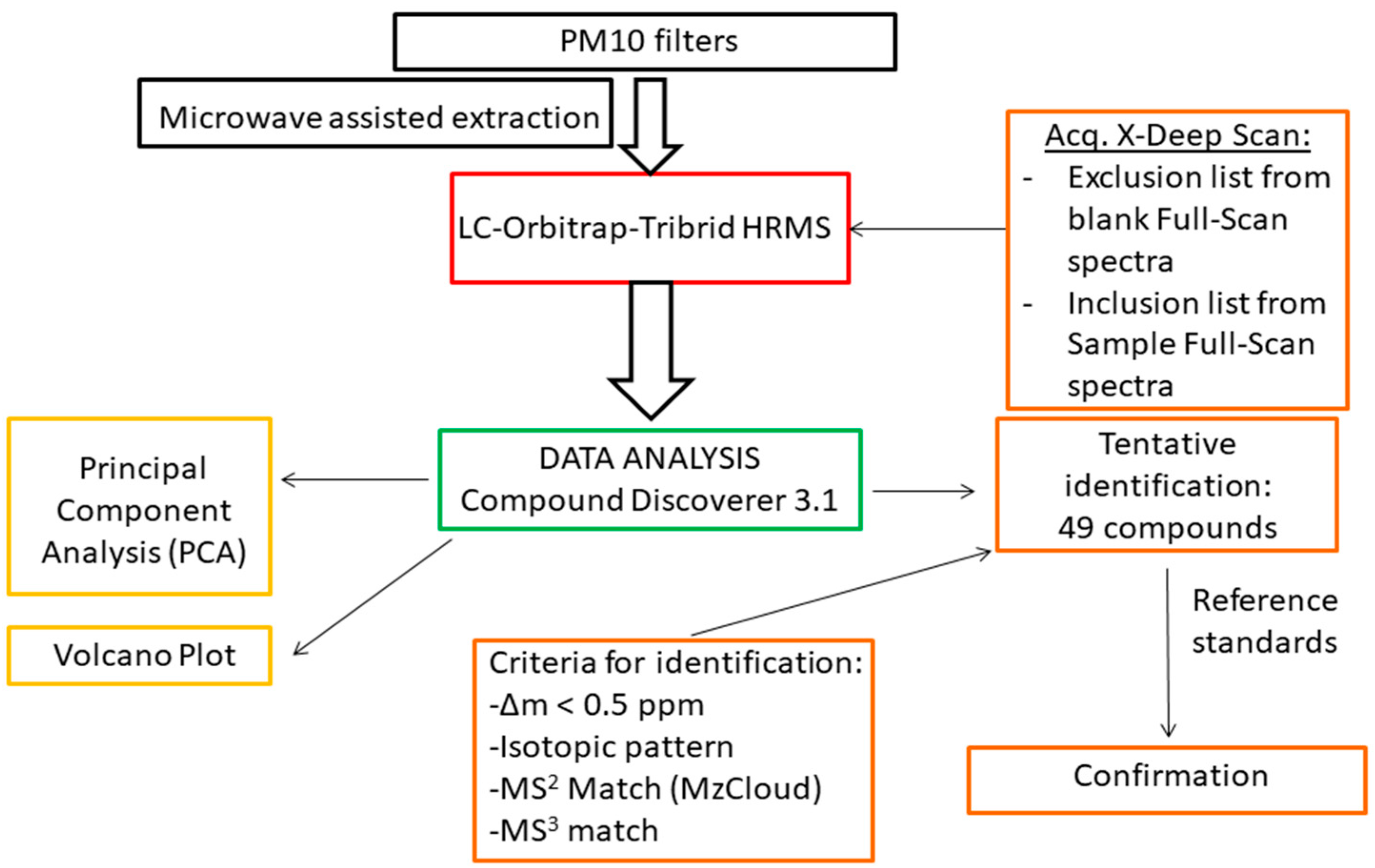
2.5. Acquisition Workflow for Unknown Analysis

A wide range of different acquisition workflows can be achieved by the use of Orbitrap Tribrid-HRMS. In this study, the AcquireX© Data Acquisition Technology (Thermo Fisher Scientific) was used in Deep Scan (DS) mode, which automatically creates an exclusion and inclusion lists after the injection of a blank and a sample (acquired in full scan), respectively. Three iterative injections of the air samples automatically update both lists (inclusion/exclusion) which permits an in-depth acquisition of the relevant features, excluding those present in the blank [29,42].

2.6. Data Processing

To be able to tentatively identify the chemicals, post-acquisition data processing was performed. Raw files were processed by CD TM 3.1 (Thermo Fisher Scientific). Mass Frontier TM 8.1 has been used in order to confirm MS3 spectra. Figure S1 shows the general workflow employed in the Orbitrap-tribrid system, and Table S1 provides a description of each node and Figure S2 illustrates the CD workflow.
In addition, CD has been employed for the statistical analysis. The data were analysed by PCA to compare the differences between the studied areas. PCA is the most commonly used approach to reduce the number of variables of a dataset while preserving as much information as possible [43]. PCA enables to explore differences between samples collected in different areas.
Moreover, a Volcano plot was performed to observe the more relevant substances in each area. A volcano plot is a type of scatter plot for replicate data that shows statistical significance (p-value) versus magnitude of change (log2Fold measures how much a variable has changed between the two measurements). In this plot, the x axis represents the log2Fold between two samples groups (generated ratio), and the y axis represents the negative log10 of the p-value (test of significance) of the fold change. Compounds in the volcano plot showing a relatively low-fold change between the two different evaluated areas appear in the centre of the plot (few differences between the two compared areas) while compounds that have significant differences between the compared areas are found in the upper-left (more likely to be found in industrial/urban areas) or the upper-right (more likely in rural areas) [44]. The following parameters were employed in order to construct the Volcano plot: p-value = 0.001 and log2Fold = 3.

2.7. Identification Criteria

In order to identify substances in the analysed samples, different levels of substance identification were considered following the criteria described by Yusà et al., (2020) [29].
The criteria used for the different levels of identification confidence were the following: predicted composition, exact mass, isotope pattern, MS2 and MS3 spectra match and RT (min). Taking into account these parameters, five different levels were defined (see Table 2) depending on the compliance of the identified substances with the identification criteria. The substances identified at Level 1 in the different Volcano plots have been compared with analytical reference standards, when these were available. In a second injection, concentrations in the ambient air (pg m−3) for these substances were estimated using the response of their analytical standards. The resulting one-point calibration (corresponding to 66 pg m−3) on identified compounds yielded semi-quantitative concentrations. This approach gives only approximate concentrations, because the purpose of the study is basically to identify and if possible confirm substances but not an accurate quantification method.
For the other 38 substances identified at Level 1, concentrations in the atmosphere (pg m−3) were estimated taking into account the average response factor of the seven substances employed in the QCRM (see average factor in Table S2).

2.8. Quality Assurance/Quality Control

To show the robustness of the developed methodology, some aspects have been assessed.
(i)
Instrument drift was monitored by analysing the areas of QCRM in the batch. Coefficient of variation (CV (%)) should be lower than 30%.
(ii)
To assure the unbiased of the methodology, all samples were injected in the same batch, sample injections were randomized, and sample preparation was performed the same day [45].
(iii)
Blank samples results were checked in order to assure that the exclusion list acquired did not contain any contamination.
(iv)
The batch acquired in CD was checked to assure that the seven substances added in the QCRM were identified.

3. Results and Discussion

The fifteen samples (5 from each area) were analysed according to the workflow described in Figure 1. After the instrumental analysis, the acquired analytical data (raw data) were processed for the following: (i) identification of unknown substances and (ii) multivariate analysis (PCA) and Volcano plot.

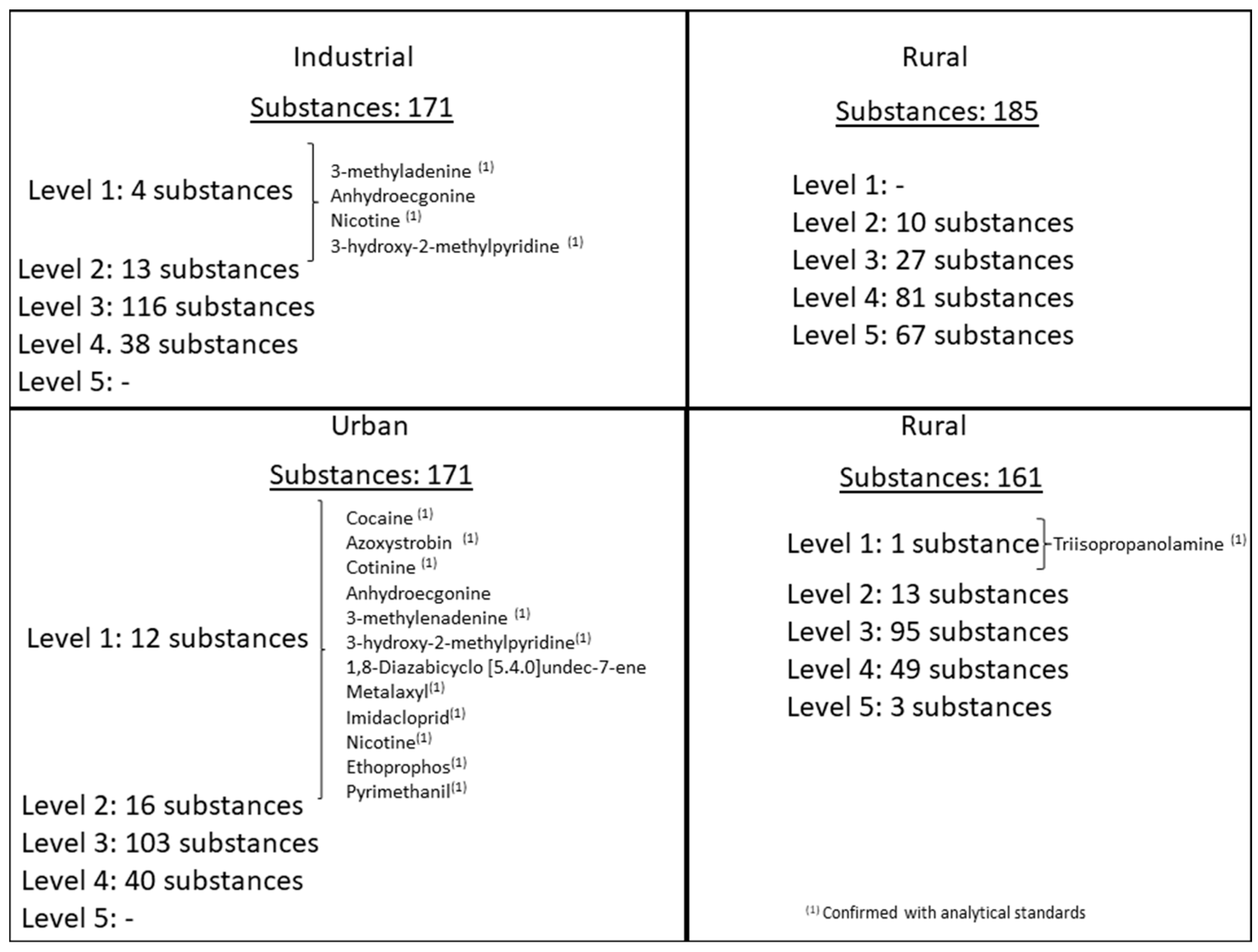
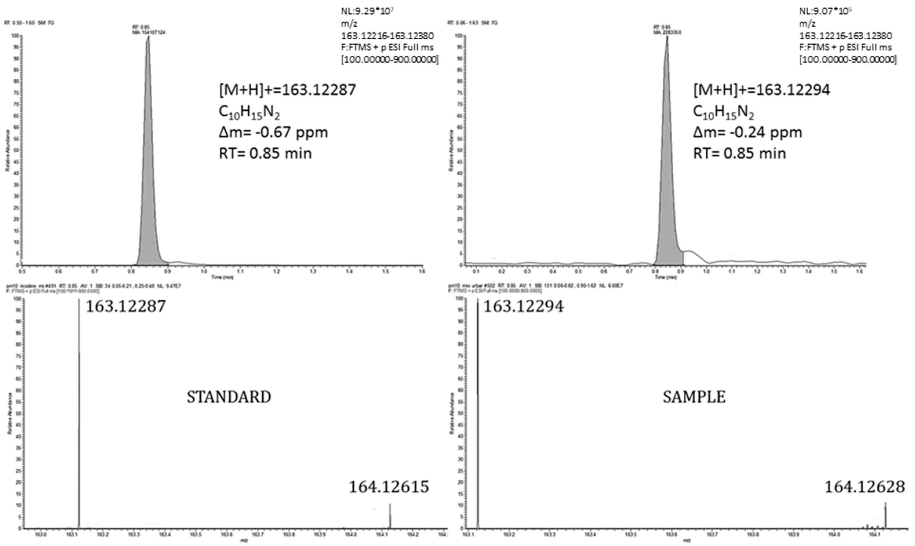
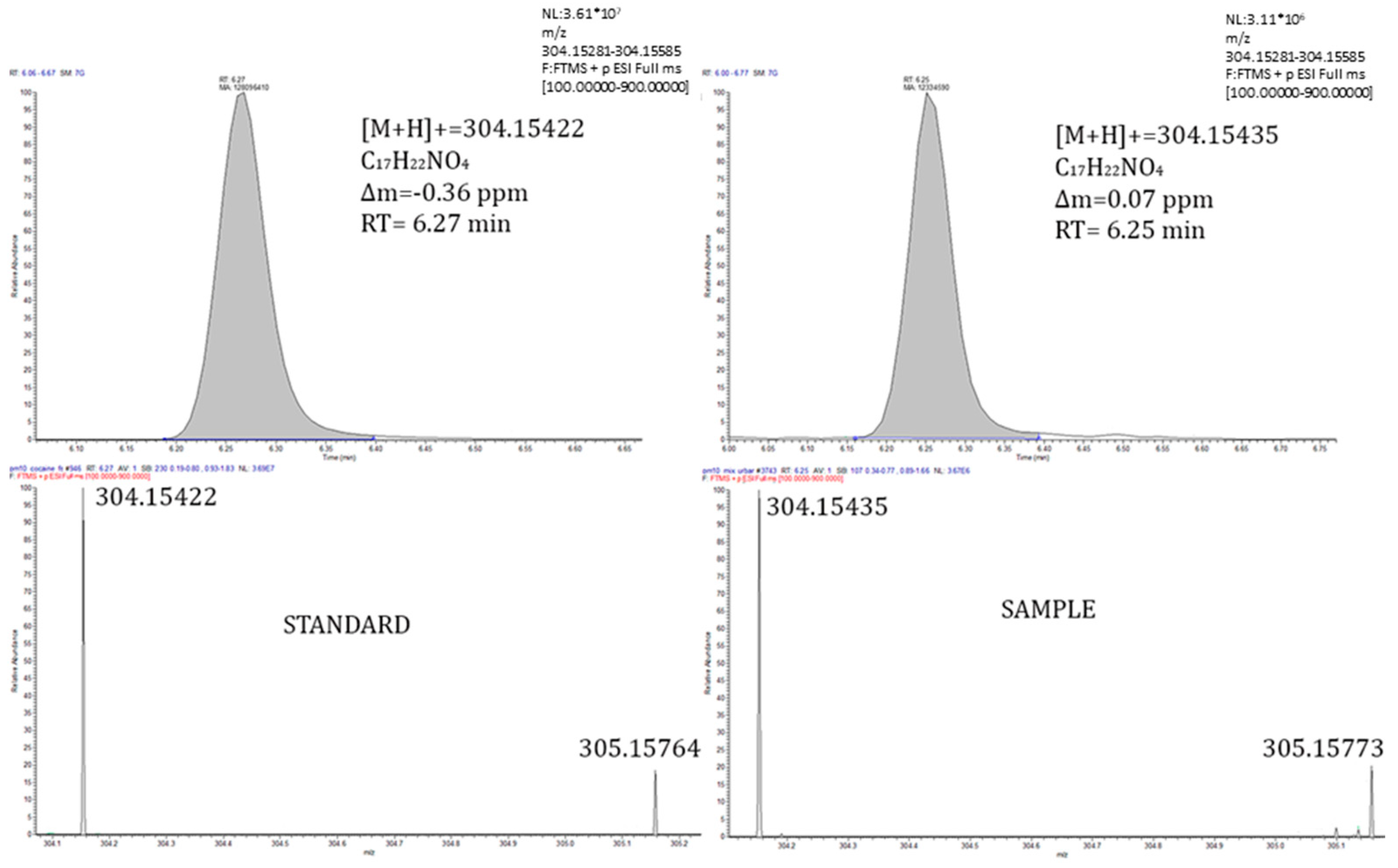
3.1. Identification of Unknown Substances

Using the employed workflow, a total of 2528 features were automatically annotated (see Figure S2). These features were classified into five different levels taking into account the identification criteria (see Table 2): 49 features met the criteria to be considered the highest confidence level (Level 1), 52 features were identified with a high confidence level (Level 2) and 1011 features were identified in level 3; meanwhile, 920 substances were tentatively identified in level 4 and 496 features were tentatively identified with the lowest confidence level (Level 5).
The experimental retention time (RT) was compared with the predicted RT considering log Kow [46] for each substance, using a known set of 116 analytical reference standards (see Table S3 and Figure S3). In most cases (more than 80%), the difference between the experimental retention time for the tentatively identified compounds and the predicted retention time was lower than 2 min.
Moreover, given that MS3 has been employed in our study and CD only automatically compares the acquired MS2 spectra with those included in the database (MzCloud) to perform the tentative identification, MS3 data need to be manually checked to increase the confidence of our results [47]. Ten out of the 49 identified substances did not have available MS3 acquired spectra in CD. Consequently, the experimental spectrum of the other 39 identified substances was compared with the available MS3 spectrum in MzCloud. For those compounds that did not have MS3 spectra in MzCloud, the theoretical in silico fragmentation performed with CD was compared with the experimental spectra. A total of 27 out of the 39 substances were successfully identified at the MS3 level.
Table S4 shows the 49 identified substances at the highest level of confidence (Level 1), which belong to different types of compounds such as pesticides, pharmaceutical active compounds, drugs, plasticizers or metabolites. While some of them had been previously detected in the ambient air, there were others which, as far as we know, have not been previously detected in the ambient air. In order to confirm that the developed methodology is suitable to identify unknown compounds, the discriminant substances detected in Section 3.2 (3-methyladenine, 3-hydroxy-2-methylpyridine, azoxystrobin, cocaine, cotinine, ethoprophos, imidacloprid, metalaxyl-M, nicotine, pyrimethanil and triisopropanolamine) were checked with their analytical reference standards. All of them were confirmed.

3.2. Differences between Areas

The acquisition in full-scan mode allowed us to obtain an individual footprint for each evaluated sample [48,49].
A PCA of the analysed samples was carried out. Figure 2 shows that the PCA model clearly enabled air samples collected in the different sampling sites to be separated. These differences imply different pollutant profiles for the assessed areas (industrial, urban and rural).
In a second step, the differences between each area (industrial, rural and urban) were assessed by comparing them in pairs to determine which substances have the greatest power of discrimination among the studied areas. In both cases, rural samples were used as reference. The substances with the greatest power of discrimination were classified according to the confidence level of their identification (see Table 2). Substances classified as Level 1 were compared with an analytical reference standard, when available so as to confirm their identification. Figure 3 summarizes the results obtained in the different Volcano plots.
Thus, taking into account the results obtained in the volcano plot where industrial samples versus rural samples were compared (see Figure S4), 171 substances (located in the upper-left) were more likely to be present in industrial areas (Table S5) while 185 compounds (located in the upper-right) were more likely to be found in rural areas (Table S6).
Four out of the 171 substances more likely to be present in industrial areas were classified as Level 1. Three of them were confirmed with their analytical standard (3-methyladenine, 3-hydroxy-2-methylpyridine and nicotine), and one of them (anhydroecgonine) was not possible to confirm because the analytical standard was unavailable. Nicotine was previously detected in the ambient air of certain urban and industrial areas: the urban atmosphere of Algiers [50]; industrial and urban areas in the National Territory Capital of Delhi in India [51] and the urban atmosphere of cities such as Amsterdam, London and Stockholm [52]. 3-methyladenine is an inhibitor of phosphatidylinositol 3-kinases (PI3K) and also has a role as a human metabolite [53], and 3-hydroxy-2-methylpyridine is an intermediate in the vitamin B6 metabolism [54]. To our knowledge, neither of these two substances has been previously identified in the ambient air. Figure 4 illustrates the chromatographic confirmation for nicotine, while in Figure S5 and Figure S6, the chromatographic confirmations for 3-methyladenine and 3-hydroxy-2-methylpyridine are shown.
Regarding the compounds more likely to be detected in rural areas, none of those detected compounds were identified at the highest confidence level (Level 1).
In the volcano plot obtained between urban and rural samples (see Figure S7), 171 compounds (in the upper-left) were classified as being more probable detected in urban areas (see Table S7), and 161 compounds (in the upper-right) were classified as more likely in rural areas (Table S8).
Twelve out of the 171 compounds classified as more probable in urban areas were identified with the highest level of confidence (Level 1). Ten out of twelve substances were confirmed using analytical standards: 3-hydroxy-2-methylpyridine, 3-methyladenine, azoxystrobin, cocaine, cotinine, ethoprophos, imidacloprid, metalaxyl, nicotine and pyrimethanil. However, two other compounds, (anhydroecgonine and 1,8-diazabicyclo [5.4.0] undec-7-ene) could not be confirmed because the analytical standards were unavailable.
Cocaine was also detected in the atmosphere of certain major cities such as Amsterdam, London [52] and Barcelona [55]. Cotinine, the most important metabolite of nicotine, was detected in urban samples. Taking into account that nicotine (its parent) has been found in some urban and industrial areas around the world, [50,51,52], it is likely that cotinine is present in urban areas. Figure 4 (nicotine), Figure 5 (cocaine) and Figure S8 (cotinine) show the confirmation of these compounds.
In this study, certain pesticides such as azoxystrobin, ethoprophos, imidacloprid, metalaxyl and pyrimethanil were identified and confirmed. These pesticides have been already detected in our region in previous studies [6]. Moreover, pyrimethanil was detected in the same urban area studied in an earlier study carried out by our research group. The detected semi-quantified levels in the present study are higher (21.84 pg m−3 vs. 8.00 pg m−3) than the ones found in our previous study [6]. Figures S9–S13 show the chromatographic confirmation of the detected pesticides.
Concerning the compounds that are more likely to be found in rural areas, one of them (triisopropanolamine) was confirmed with their analytical standard (see Figure S14) and then classified as Level 1. Triisopropanolamine is widely used as emulsifier, stabilizer, surfactant and chemical intermediate. One of its main applications of triisopropanolamine is to neutralize pesticides [56].

4. Study Limitations

Samples were collected in only one season, and there may be differences in the particulate phase at different seasons of the year.
In some cases, it could be difficult to classify in only one group a sampling area that should be part of more than one group.
Regarding structural elucidation, the detection of isomers is not possible, and we should use other techniques (for instance, nuclear magnetic resonance).

5. Conclusions

A novel analytical approach has been developed in order to identify unknown compounds in PM10 ambient air. This strategy enables the tentative identification of 49 compounds, belonging to different chemical groups such as pesticides, pharmaceutical products, drugs, plasticizers and metabolites. Furthermore, when applying it, the use of MS3 showed better structural elucidation for the detected compounds.
Different profiles were obtained for rural, urban and industrial areas, and since, each area has a specific footprint, different organic pollutants were detected.
When industrial and rural areas were compared, three substances were confirmed in industrial areas: 3-methyladenine, nicotine and 3-hydroxy-2-methylpyridine. In the comparison of urban and rural areas, 10 substances were detected in urban areas: 3-hydroxy-2-methylpyridine, 3-methyladenine, azoxystrobin, cocaine, cotinine, ethoprophos, imidacloprid, metalaxyl, nicotine and pyrimethanil whereas the presence of one substance (triisopropanolamine) was confirmed in rural areas.
This strategy could be implemented as an analytical tool in future studies related to Air Quality projects worldwide. Moreover, it may provide useful information about unknown compounds (regulated or not) which can be detected in the ambient air by LC-HRMS.

Supplementary Materials

The following supporting information can be downloaded at: https://www.mdpi.com/article/10.3390/toxics10050220/s1. Table S1: Description of the different nodes of the CD workflow; Table S2: Average response factor of internal standard; Table S3: Table of Log Kow vs. Retention time (RT) of the analytical reference standards; Table S4: Identified compounds and spectrometric and chromatographic criteria; Table S5: Compounds more probably present in industrial areas (Industrial-Rural); Table S6: Compounds more probably present in rural areas (Industrial-Rural); Table S7: Compounds more probably present in urban areas (Urban-Rural); Table S8: Compounds more probably present in rural areas (Urban-Rural); Figure S1: Workflow used in AcquireX Deep Scan Mode-MS3; Figure S2: Workflow used in Compound Discoverer™ data processing; Figure S3: Graphic of Log Kow vs. Retention time (RT) of the analytical reference standards; Figure S4: Volcano plot for identification of discriminating substances between industrial and rural areas (employed parameters: p-value = 0.001 and log2Fold = 3); Figure S5: 3-methyladenine; Figure S6: 3-hydroxy-2-methylpyridine; Figure S7: Volcano plot for identification of discriminating substances between urban and rural areas (employed parameters: p-value = 0.001 and log2Fold = 3); Figure S8: Cotinine; Figure S9: Azoxystrobin; Figure S10: Ethoprophos; Figure S11: Imidacloprid; Figure S12: Metalaxyl; Figure S13: Pyrimethanil; Figure S14: Triisopropanolamine.

Author Contributions

Conceptualization, V.Y.; methodology, A.L.; validation, A.L.; resources, A.L., E.F.; writing—original draft preparation, A.L.; writing—review and editing, E.F., V.Y., M.I. and C.C.; supervision, V.Y., M.I. and C.C. All authors have read and agreed to the published version of the manuscript.

Funding

This work is the result of the RISKAIR project “Air Quality in the Valencian Region: development of new methodologies for the determination of emerging pollutants and risk assessment” (UGP-20-309). It was funded by the UJI-FISABIO Calls for preparatory actions to support the exploration and formulation of future research or innovation coordinated by researchers from the Universitat Jaume I (UJI) and the Foundation of the Promotion of Health and Biomedical research of the Valencian Region (FISABIO). The European Commission financed the analytical instruments used here through the European Regional Development Funds (ERDF) Operational Programme of the Valencian Region (2014–2020).

Conflicts of Interest

The authors declare no conflict of interest.

References

  1. Popescu, F.; Ionel, I. Anthropogenic Air Pollution Sources. In Air Quality; Kumar, A., Ed.; InTech: New Dehli, India, 2010. [Google Scholar] [CrossRef] [Green Version]
  2. Safieddine, S.A.; Heald, C.L.; Henderson, B.H. The global nonmethane reactive organic carbon budget: A modeling perspective. Geophys. Res. Lett. 2017, 44, 3897–3906. [Google Scholar] [CrossRef] [Green Version]
  3. Woodrow, J.E.; Gibson, K.E.; Seiber, J.N. Pesticides and related toxicants in the atmosphere. Part Rev. Environ. Contam. Toxicol. Book Ser. 2018, 247, 147–196. [Google Scholar] [CrossRef]
  4. Jimenez, J.L.; Canagaratna, M.R.; Donahue, N.M.; Prevot, A.S.H.; Zhang, Q.; Kroll, J.H.; DeCarlo, P.F.; Allan, J.D.; Coe, H.; Ng, N.L.; et al. Evolution of Organic Aerosols in the Atmosphere. Science 2009, 326, 1525–1529. [Google Scholar] [CrossRef] [PubMed]
  5. Alburquerque, M.; Coutinho, M.; Borrego, C. Long-term monitoring and seasonal analysis of polycyclic aromatic hydrocarbons (PAHs) measured over a decade in the ambient air of Porto, Portugal. Sci. Total Environ. 2016, 543, 439–448. [Google Scholar] [CrossRef] [PubMed]
  6. López, A.; Yusà, V.; Muñoz, A.; Vera, T.; Borràs, E.; Ródenas, M.; Coscollà, C. Risk assessment of airborne pesticides in a Mediterranian Region of Spain. Sci. Total Environ. 2017, 574, 724–734. [Google Scholar] [CrossRef]
  7. López, A.; Coscollà, C.; S-Hernández, C.; Pardo, O.; Yusà, V. Dioxins and dioxin-like PCBs in the ambient air of the Valencian Region. Levels, human exposure and risk assessment. Chemosphere 2021, 267, 128902. [Google Scholar] [CrossRef]
  8. Beser, M.I.; Beltrán, J.; Yusà, V. Design of experiment approach for the optimization of polybrominated diphenyl ethers determination in fine airborne particulate matter by microwave-assisted extraction and gas chromatography coupled to tandem mass spectrometry. J. Chromatogr. A 2014, 1323, 1–10. [Google Scholar] [CrossRef]
  9. Thurston, G.; Ahn, J.; Cromar, K.; Shao, Y.; Reynolds, H.; Jerrett, M.; Lim, C.; Shanley, R.; Park, Y.; Hayes, R. Ambient particulate matter air pollution exposure and mortality in the NIH-AARP Diet and Health Cohort. Environ. Health Perspect. 2016, 124, 484–490. [Google Scholar] [CrossRef]
  10. Zhang, C.; Ding, R.; Xiao, C.C.; Xu, Y.C.; Cheng, H.; Zhu, F.R.; Lei, R.Q.; Di, D.S.; Zhao, Q.H.; Cao, J.Y. Association between air pollution and cardiovascular mortality in Hefei, China: A time-series analysis. Environ. Pollut. 2017, 229, 790–797. [Google Scholar] [CrossRef]
  11. Hu, C.Y.; Huang, K.; Fang, Y.; Yang, X.J.; Ding, K.; Jiang, W.; Hua, X.G.; Huang, D.Y.; Jiang, Z.X.; Zhang, X.J. Maternal air pollution exposure and congenital heart defects in offspring: A systematic review and meta-analysis. Chemosphere 2020, 253, 126668. [Google Scholar] [CrossRef]
  12. Harner, T.; Bidleman, T.F. Octanol-Air Partition Coefficient for describing particle/gas partitioning of aromatic compounds in urban air. Environ. Sci. Technol. 1998, 32, 1494–1502. [Google Scholar] [CrossRef]
  13. Lee, R.M.G.; Jones, K.C. Gas-particle partitioning of atmospheric PCDD/Fs: Measurements and observations on modeling. Environ. Sci. Technol. 1998, 33, 3596–3604. [Google Scholar] [CrossRef]
  14. Esen, F.; Tasdemir, Y.; Vardar, N. Atmospheric concentrations of PAHs, their possible sources and gas-to-particle partitioning at a residential site of Bursa, Turkey. Atmos. Res. 2008, 88, 243–255. [Google Scholar] [CrossRef]
  15. Gamble, J.F.; Lewis, R.J. Health and respirable particulate (PM10) air pollution: A causal or statistical association? Environ. Health Perspect. 1996, 104, 838–850. [Google Scholar] [CrossRef] [PubMed]
  16. Liu, A.; Wijesiri, B.; Hong, N.; Zhu, P.; Egodawatta, P.; Goonetillleke, A. Understanding re-distribution of road deposited particle-bound pollutants using a Bayesian Network (BN) approach. J. Hazard. Mater. 2018, 355, 56–64. [Google Scholar] [CrossRef]
  17. Lenschow, P.; Abraham, H.J.; Kutzner, K.; Lutz, M.; Pruß, J.D.; Reichenbächer, W. Some ideas about the sources of PM10. Atmos. Environ. 2001, 35 (Suppl. S1), S23–S33. [Google Scholar] [CrossRef]
  18. Putaud, J.-P.; Van Dingenen, R.; Alastuey, A.; Bauer, H.; Birmili, W.; Cyrys, J.; Flentje, H.; Fuzzi, S.; Gehrig, R.; Hansson, H.C.; et al. A European aerosol phenomenologye: Physical and chemical characteristics of particulate matter from 60 rural, urban, and kerbside sites across Europe. Atmos. Environ. 2004, 44, 1308–1320. [Google Scholar] [CrossRef]
  19. Bathmanabhan, S.; Saragur-Madanayak, S.N. Analysis and interpretation of particulate matter-PM10, PM2.5 and PM1 emissions from the hetergoneous traffic near an urban roadway. Atmos. Pollut. Res. 2010, 1, 184–194. [Google Scholar] [CrossRef] [Green Version]
  20. Chuturkova, R. Particulate matter air pollution (PM10 and PM2.5) in urban and industrial areas. J. Sci. Educ. Innov. 2015, 5, 13–32. [Google Scholar]
  21. Zhang, W.; Wang, J.; Xu, Y.; Wang, C.; Streets, D.G. Analyzing the spatio-temporal variation of the CO2 emissions from district heating systems with “Coal-to-Gas” transition: Evidence from GTWR model and satellite data in China. Sci. Total Environ. 2022, 803, 150083. [Google Scholar] [CrossRef]
  22. EEA. Air Quality in Europe-2012 Report. In European Environmental Agency Report. No 4/2012; EEA: Copenhagen, Denmark, 2012. [Google Scholar]
  23. Harner, T.; Shoeib, M.; Diamond, M.; Stern, G.; Rosenberg, B. Using passive air samplers to assess Urban-Rural trends for Persistent Organic Pollutants. Polychlorinated Biphenyls and Organochlorine Pesticides. Environ. Sci. Technol. 2004, 38, 4474–4483. [Google Scholar] [CrossRef] [PubMed]
  24. Guéguen, F.; Stille, P.; Millet, M. Persistent organic pollutants in the atmosphere from urban and industrial environments in the Rhine Valley: PCBs, PCDD/Fs. Environ. Sci. Pollut. Res. Int. 2013, 20, 3852–3862. [Google Scholar] [CrossRef] [PubMed]
  25. Zhang, W.; Lu, Z.; Xu, Y.; Wang, C.; Gu, Y.; Xu, H.; Streets, D.G. Black carbon emissions from biomass and coal in rural China. Atmos. Environ. 2018, 176, 158–170. [Google Scholar] [CrossRef]
  26. Lucci, P.; Saurina, J.; Núñez, A. Trends in LC-MS and LC-HRMS analysis and characterization of polyphenols in food. Trac-Trends Anal. Chem. 2016, 88, 1–24. [Google Scholar] [CrossRef] [Green Version]
  27. Martinez-Bueno, M.J.; Gomez Ramos, M.J.; Bauer, A.; Fernandez-Alba, A.R. An overview of non-targeted screening strategies based on high resolution accurate mass spectrometry for the identification of migrants coming from plastic food packaging materials. Trac-Trends Anal. Chem. 2019, 110, 191–203. [Google Scholar] [CrossRef]
  28. Yusop, A.Y.M.; Xiao, L.; Fu, S. Determination of phosphodiesterase 5 (PDE5) inhibitors in instant coffee premixes using liquid chromatography-high-resolution mass spectrometry (LC-HRMS). Talanta 2019, 204, 36–43. [Google Scholar] [CrossRef]
  29. Yusà, V.; López, A.; Dualde, P.; Pardo, O.; Fochi, I.; Pineda, A.; Coscollà, C. Analysis of unknowns in recycled LDPE plastic by LC-Orbitrap Tribrid HRMS using MS3 with an intelligent data acquisition mode. Microchem. J. 2020, 158, 1052526. [Google Scholar] [CrossRef]
  30. Liu, A.; Qu, G.; Zhang, C.; Gao, Y.; Shi, J.; Du, Y.; Jiang, G. Identification of two novel brominated contaminants in water samples by ultra-high performance liquid chromatography-Orbitrap Fusion Tribrid mass spectrometer. J. Chromatogr. A 2015, 1377, 92–99. [Google Scholar] [CrossRef]
  31. Wu, Y.; Gao, S.; Liu, Z.; Zhao, J.; Ji, B.; Zeng, X.; Yu, Z. The quantification of chlorinated paraffins in environmental samples by ultra-high-performance liquid chromatography coupled with Orbitrap Fusion Tribrid mass spectrometry. J. Chromatogr. A 2019, 1593, 102–109. [Google Scholar] [CrossRef]
  32. Thermo Scientific. SN65392-EN 0119M. AcquireX, 2019. Available online: https://www.thermofisher.com/es/es/home/industrial/mass-spectrometry/liquid-chromatography-mass-spectrometry-lc-ms/lc-ms-software/lc-ms-data-acquisition-software/acquirex-intelligent-data-acquisition-workflow.html (accessed on 18 June 2020).
  33. Thermo Scientific. 2019. Available online: https://www.thermofisher.com/es/es/home/industrial/mass-spectrometry/liquid-chromatography-mass-spectrometry-lcms/lc-ms-software/multi-omics-data-analysis/compound-discoverer-software.html (accessed on 16 June 2020).
  34. López, A.; Yusà, V.; Millet, M.; Coscollà, C. Retrospective screening of pesticide metabolites in ambient air using liquid chromatography coupled to high-resolution mass spectrometry. Talanta 2016, 150, 27–36. [Google Scholar] [CrossRef]
  35. Brüggemann, M.; van Pinxteren, D.; Wang, Y.; Yu, J.Z.; Herrmann, H. Quantification of known and unknown terpenoid organosulfates in PM10 using untargeted LC-HRMS/MS: Contrasting summertime rural Germany and the North China Plain. Environ. Chem. 2019, 16, 333–346. [Google Scholar] [CrossRef] [Green Version]
  36. Spranger, T.; van Pixteren, D.; Reemtsma, T.; Lechtenfeld, O.J.; Hermann, H. 2D Liquid chromatographic fractionation with ultra-high resolution MS analysis resolves a vast molecular diversity of trophospheric particle organics. Environ. Sci. Technol. 2019, 53, 11353–11363. [Google Scholar] [CrossRef] [PubMed]
  37. Han, L.; Kaesler, J.; Peng, C.; Reemtsma, T.; Lechtenfeld, O.J. Online Counter Gradient LC-FT-ICR-MS Enables Detection of Highly Polar Natural Organic Matter Fractions. Anal. Chem. 2021, 93, 1740–1748. [Google Scholar] [CrossRef] [PubMed]
  38. Pereira, K.L.; Ward, M.W.; Wilkinson, J.L.; Sallach, J.B.; Bryant, D.J.; Dixon, W.J.; Hamilton, J.F.; Lewis, A.C. An Automated Methodology for Non-targeted Compositional Analysis of Small Molecules in High Complexity Environmental Matrices Using Coupled Ultra Performance Liquid Chromatography Orbitrap Mass Spectrometry. Environ. Sci. Technol. 2021, 55, 7365–7375. [Google Scholar] [CrossRef] [PubMed]
  39. Chung, I.Y.; Park, Y.M.; Lee, H.J.; Kim, H.; Kim, D.H.; Kim, I.G.; Kim, S.M.; Do, Y.S.; Seok, K.S.; Kwon, J.H. Nontarget screening using passive air and water sampling with a level II fugacity model to identify unregulated environmental contaminants. Int. J. Environ. Sci. 2017, 62, 84–91. [Google Scholar] [CrossRef] [PubMed]
  40. Dubocq, F.; Bjurlid, F.; Ydstal, D.; Titaley, I.A.; Reiner, E.; Wang, T.; Ortiz-Almirall, X.; Kärrman, A. Organic contaminants formed during fire extinguishing using different firefighting methods assessed by nontarget analysis. Environ. Pollut. 2020, 265, 114834. [Google Scholar] [CrossRef] [PubMed]
  41. Zhang, X.; Saini, A.; Hao, C.; Harner, T. Passive air sampling and nontargeted analysis for screening POP-like chemicals in the atmosphere: Opportunities and challenges. Trends Anal. Chem. 2020, 132, 116052. [Google Scholar] [CrossRef]
  42. Yusà, V.; López, A.; Dualde, P.; Pardo, O.; Fochi, I.; Miralles, P.; Coscollà, C. Identification of 24 Unknown Substances (NIAS/IAS) from Food Contact Polycarbonate by LC-Orbitrap Tribrid HRMS-DDMS3: Safety Assessment. Int. J. Anal. Chem. 2021, 2021, 6654611. [Google Scholar] [CrossRef]
  43. Jolliffe, I.T.; Cadima, J. Principal component analysis: A review and recent developments. Philos. Trans. R. Soc. A 2016, 374, 20150202. [Google Scholar] [CrossRef]
  44. Hur, M.; Campbell, A.A.; Almeida-de-Macedo, M.; Li, L.; Ransom, N.; Jose, A.; Crispin, M.; Nikolau, B.J.; Wurtele, E.S. A global approach to analysis and interpretation of metabolic data for plant natural product discovery. Nat. Prod. Rep. 2013, 30, 565–583. [Google Scholar] [CrossRef] [Green Version]
  45. Broadhurst, D.; Goodacre, R.; Reinke, S.N.; Kuligowski, J.; Wilson, I.D.; Lewis, M.R.; Dunn, W.B. Guidelines and considerations for the use of system suitability and quality control samples in mass spectrometry assays applied in untargeted clinical metabolomic studies. Metabolomics 2018, 14, 72. [Google Scholar] [CrossRef] [PubMed] [Green Version]
  46. Chemspider Webpage. 2021. Available online: http://www.chemspider.com/ (accessed on 31 July 2021).
  47. Thermo Fisher Scientific. Mass Frontier Spectral Interpretation Software. Available online: https://www.thermofisher.com/es/es/home/industrial/mass-spectrometry/liquid-chromatography-mass-spectrometry-lc-ms/lc-ms-software/multi-omics-data-analysis/mass-frontier-spectral-interpretation-software.html (accessed on 19 October 2020).
  48. Katajamaa, M.; Orseic, M. Data processing for mass spectrometry-based metabolomics. J. Chromatogr. A 2007, 1158, 318–328. [Google Scholar] [CrossRef] [PubMed]
  49. López, A.; Dualde, P.; Yusà, V.; Coscollà, C. Retrospective analysis of pesticide metabolites in urine using liquid chromatography coupled to high-resolution mass spectrometry. Talanta 2016, 160, 547–555. [Google Scholar] [CrossRef]
  50. Ladji, R.; Yassaa, N.; Balducci, C.; Cecinato, A.; Meklati, B.Y. Annual variation of particulate organic compounds in PM10 in the urban atmosphere of Algiers. Atmos. Res. 2009, 92, 258–269. [Google Scholar] [CrossRef]
  51. Yadav, S.; Tandom, A.; Attri, A.K. Timeline trend profile and seasonal variations in nicotine present in ambient PM10 samples: A four year investigation from Delhi region, India. Atmos. Environ. 2014, 98, 89–97. [Google Scholar] [CrossRef]
  52. Balducci, C.; Green, D.C.; Romagnoli, P.; Perilli, M.; Johansson, C.; Panteliadis, P.; Cecinato, A. Cocaine and cannabinoids in the atmosphere of Northern Europe cities, comparison with Southern Europe. Env. Int. 2016, 97, 187–194. [Google Scholar] [CrossRef] [Green Version]
  53. Dai, S.; Wang, B.; Li, W.; Wang, L.; Song, X.; Guo, C.; Li, Y.; Liu, F.; Zhu, F.; Wang, Q.; et al. Systemic application of 3-methyladenine markedly inhibited atherosclerotic lesion in ApoE-/- mice by modulation autophagy, foam cell formation and immune-negative molecules. Cell Death Dis. 2016, 7, e2498. [Google Scholar] [CrossRef] [Green Version]
  54. Schterev, I.G.; Delchev, V.B. Excited state deactivation channels via internal conversions in two positions isomers of hydroxyl-methyl-pyridine: A theoretical study. J. Phys. Org. Chem. 2015, 28, 681–689. [Google Scholar] [CrossRef]
  55. Mastroianni, N.; Postigo, C.; López de Alda, M.; Viana, M.; Rodríguez, A.; Alastuey, A.; Querol, X.; Barceló, D. Comprehensive monitoring of the occurrence of 22 drugs and transformation products in airborne particulate matter in the city of Barcelona. Sci. Total Environ. 2015, 532, 344–352. [Google Scholar] [CrossRef]
  56. Singh, G.; Saroa, A.; Girdhar, S.; Rani, S.; Choquesillo-Lazarte, D.; Chandra-Sahoo, S. Incorporation of azo group at axial position of silatranes: Synthesis, characterization and antimicrobial activity. Appl. Organometal. Chem. 2015, 29, 549–555. [Google Scholar] [CrossRef]
Figure 1. Workflow of the different steps of the study.
Toxics 10 00220 g001
Figure 2. Two dimensional PCA score plot of air samples for industrial, rural and urban areas.
Toxics 10 00220 g002
Figure 3. Obtained results in the Volcano plots (industrial vs. rural and urban vs. rural).
Toxics 10 00220 g003
Figure 4. Extracted ion chromatogram (top) and isotopic profile (bottom) corresponding to the protonated molecule of nicotine in a standard (left) and a real sample (right).
Toxics 10 00220 g004
Figure 5. Extracted ion chromatogram (top) and isotopic profile (bottom) corresponding to the protonated molecule of cocaine in a standard (left) and a real sample (right).
Toxics 10 00220 g005
Table 1. Description of sampling sites of PM10 samples.
Sampling SiteLatitudeLongitudeDescription
Burriana39°53′52″0°03′54″Rural and agricultural area surrounded by citrus groves (orange trees). Samples collected about 20 m above sea level.
Onda39°57′46″0°15′00″Industrial area. Samples collected about 160 m above sea level.
Valencia-Viveros39°28′46″0°22′10″Commercial and urban area and inside a park (Viveros) with gardens. Samples collected at 11 m above sea level.
Table 2. Levels of confidence and criteria used for tentative identification.
LevelParameterCriteria
Level 1Molecular formula (Predicted composition) 1Full match
∆ mass (ppm) 2<0.5 ppm
Isotope profile (SFit) 3>70%
MzCloud Match 4>70%
MS2 Data 5Yes
RT (min)Consistent with the predicted RT (min) (±2 min)/analytical standard *
Level 2Molecular formula (Predicted composition) 1Full match
∆ mass (ppm) 2<0.5 ppm
Isotope profile (SFit) 350–70%
MzCloud Match 450–70%
MS2 Data 5Yes
RT (min)Consistent with the predicted RT (min) (±2 min)
Level 3Molecular formula (Predicted composition) 1Full match
∆ mass (ppm) 2<0.5 ppm
MS2 Data 5Yes
Level 4Molecular formula (Predicted composition) 1Full match
∆ mass (ppm) 2<0.5 ppm
MS2 Data 5No
Predicted substance 6Name
Level 5Molecular formula (Predicted composition) 1Full match
∆ mass (ppm) 2<0.5 ppm
MS2 Data 5No
Predicted substance 6No Name
1 Molecular formula (Predicted composition): Assigned elemental composition coincidence with a proposed substance from databases (ChemSpider, Mass List). 2 Δ mass (ppm): mass error (in ppm). 3 Isotope profile (SFit): match between the experimental isotopic pattern and the theoretical one. 4 MzCloud Match: match between the experimental and the MS2 spectra in the mzCloud library. 5 MS2 data: Match between experimental MS2 spectra and the theoretical one in CD. 6 Predicted substance: Name described in one of the employed databases: mzVault/mzCloud Library/ChemSpider/Mass List. * When analytical standard was available, the RT difference between standard and sample was compared.
Publisher’s Note: MDPI stays neutral with regard to jurisdictional claims in published maps and institutional affiliations.

