Energy Levels in Pentacoordinate d⁵ to d⁹ Complexes

Abstract

Energy levels of pentacoordinate d⁵ to d⁹ complexes were evaluated according to the generalized crystal field theory at three levels of sophistication for two limiting cases of pentacoordination: trigonal bipyramid and tetragonal pyramid. The electronic crystal field terms involve the interelectron repulsion and the crystal field potential; crystal field multiplets account for the spin–orbit interaction; and magnetic energy levels involve the orbital– and spin–Zeeman interactions with the magnetic field. The crystal field terms are labelled according to the irreducible representations of point groups D_3h and C_4v using Mulliken notation. The crystal field multiplets are labelled with the Bethe notations for the respective double groups D’₃ and C’₄. The magnetic functions, such as the temperature dependence of the effective magnetic moment and the field dependence of the magnetization, are evaluated by employing the apparatus of statistical thermodynamics as derivatives of the field-dependent partition function. When appropriate, the formalism of the spin Hamiltonian is applied, giving rise to a set of magnetic parameters, such as the zero-field splitting D and E, magnetogyric ratio tensor, and temperature-independent paramagnetism. The data calculated using GCFT were compared with the ab initio calculations at the CASSCF+NEVPT2 level and those involving the spin–orbit interaction.

1. Introduction

A correct interpretation of electronic spectra for transition metal complexes (d-d transitions), magnetometric data (magnetic susceptibility and magnetization), and spectra of electron spin resonance requires appropriate theoretical support. A traditional approach is represented by the crystal field theory, which is well elaborated for octahedral complexes (O_h symmetry), even with tetragonal (trigonal) distortion (D_4h, D_3d) [1,2,3,4,5]. Analogously, tetrahedral patterns (T_d) and their distortion daughters to prolate and/or oblate bispheoids (D_2d) are also known. However, one is rather helpless when dealing with pentacoordination in its limiting cases represented by trigonal bipyramids (D_3h) and tetragonal pyramids (C_4v) and especially for intermediate geometries on the Berry rotation path (C_2v).

A target of the present work is to elucidate a comprehensive view of the crystal field terms and crystal field multiplets in the case of pentacoordinate d⁵ to d⁹ complexes. Whereas multielectron crystal field terms are labelled according to Mulliken notation (A, B, E, T), the involvement of the spin–orbit interaction requires a passage from common symmetry point groups to double groups; therefore, crystal field multiplets are labelled according to Bethe notation (Γ₁ to Γ₈).

Geometries belonging to point groups O_h, T_d, D_4h, or D_2d are mostly omitted hereafter; numerical computer-assisted treatment is necessary when ligands occupy arbitrary positions. This approach is slightly more complicated, involving algebra of complex numbers due to the occurrence of complex spherical harmonic functions fixing the ligand positions. The treatment used below is termed the Generalized Crystal Field Theory, as outlined elsewhere [6].

The eigenvalues of the model Hamiltonian refer to the energy levels at a given approximation. The eigenvectors bear all information about the symmetry of the wave function; therefore, they can be utilized to assign irreducible representations (IRs) either of the crystal field terms $\left|d^n:(LS);G:\mathsf{\Gamma }\gamma a\right.〉$ or the crystal field multiplets $\left|d^n:(J);G^{\prime }:{\mathsf{\Gamma }}^{\prime }{\gamma }^{\prime }{a}^{\prime }\right.〉$. The irreducible representation within point group G is Γ, γ (its component when IR is degenerate), and a (the branching (repetition) number). The same holds true for double group G′.

2. Results

The generalized crystal field theory (GCFT) applied below is fully described elsewhere, along with the closed formulae for the matrix elements of the involved operators in the basis set of the electronic atomic terms $\left|\mathsf{\Psi }\right.〉=\left|d^n:\nu LS{M}_L{M}_S\right.〉$, where the apparatus of the irreducible tensor operators has been utilized [6,7]. (Here, the seniority number (ν) for the terms can distinguish between terms possessing the same set $\left\{LS\right\}$; the quantum numbers adopt their usual meaning [8]). These matrix elements refer to five operators:

(a)

Interelectronic repulsion $〈{\mathsf{\Psi }}^{\prime }\left|{\widehat{V}}_{\mathrm{ee}}\right|\mathsf{\Psi }〉$ parametrized by the Racah parameters B_M and C_M;

(b)

Crystal field potential $〈{\mathsf{\Psi }}^{\prime }\left|{\widehat{V}}_{\mathrm{cf}}\right|\mathsf{\Psi }〉$ depending upon crystal field poles (strengths) F_k(R_L) of the k-th order (k = 4, 2) for each ligand (L) and its position;

(c)

Spin–orbit interaction $〈{\mathsf{\Psi }}^{\prime }\left|{\widehat{V}}_{\mathrm{so}}\right|\mathsf{\Psi }〉$ depending upon the spin–orbit coupling constant (ξ_M);

(d)

The orbital Zeeman term $〈{\mathsf{\Psi }}^{\prime }\left|{\widehat{V}}_{\mathrm{lB}}(B)\right|\mathsf{\Psi }〉$, which eventually involves the orbital reduction factors; and

(e)

The spin Zeeman term $〈{\mathsf{\Psi }}^{\prime }\left|{\widehat{V}}_{\mathrm{sB}}(B)\right|\mathsf{\Psi }〉$, which contains the spin-only magnetogyric (g_e) factor.

The position of ligands (L) is arbitrary and fixed by the polar coordinates {${\vartheta }_L,{\phi }_L$}. The model Hamiltonian involves three important cases:

1.

Diagonalization of (a) + (b) yields the energies of crystal field terms $\left|d^n:(LS);G:\mathsf{\Gamma }\gamma a\right.〉$, which span the IRs of point group G;

2.

Diagonalization of (a) + (b) + (c) produces energies of the crystal field multiplets in the zero magnetic field $\left|d^n:(J);G^{\prime }:{\mathsf{\Gamma }}^{\prime }{\gamma }^{\prime }{a}^{\prime }\right.〉$, which span the IRs of double group G′;

3.

Diagonalization of (a) + (b) + (c) + (d) + (e) gives the magnetic energy levels in the applied magnetic field.

The energy levels of crystal field multiplets for the half-integral spin (S = 1/2, 3/2, 5/2) appear as Kramers doublets and remain doubly degenerate in the absence of a magnetic field. This is the case of high-spin Fe(III), Mn(II), Co(II), and Cu(II) complexes.

Traditional crystal field theory operates with a set of collective parameters, such as 10Dq = Δ, Ds, Dt, etc., and is useful for cases certain symmetry, such as O_h, T_d, and D_4h, all of which are derived from the crystal field poles (F₄(L) and eventually F₂(L)), e.g.,

• For O_h/D_4h: 10Dq = (10/6)F₄(xy);
• Dt = (2/21)[F₄(xy) − F₄(z)];
• Ds = (2/7) [F₂(xy) − F₂(z)]; and
• For T_d: 10Dq = (20/27)F₄(xy).

The crystal field poles originate in the partitioning of the matrix elements of the crystal field potential into radial (R) and angular (A) parts in the polar coordinates $(R_K,{\vartheta }_K,{\phi }_K)$.

$$〈{\mathsf{\Psi }}^{\prime }(R,A)\left|{\widehat{V}}_{\mathrm{cf}}(R,A)\right|\mathsf{\Psi }(R,A)〉=〈{\mathsf{\Psi }}^{\prime }(R)\left|{\widehat{V}}_{\mathrm{cf}}(R)\right|\mathsf{\Psi }(R)〉·〈{\mathsf{\Psi }}^{\prime }(A)\left|{\widehat{V}}_{\mathrm{cf}}(A)\right|\mathsf{\Psi }(A)〉$$

(1)

The integration of the angular part yields some values (manually calculated for some cases, such as O_h symmetry). This part contains the spherical harmonic functions $Y_{k,q}({\vartheta }_K,{\phi }_K)$ for the positions of ligand K, and in general, it is a complex number. The radial part contains the metal–ligand distance (R_K) and defines the crystal field poles:

$$F_k(R_K)={\displaystyle \underset{0}{\overset{\infty }{\int }}{R}_{nl}^{\ast }(r)\frac{r_{<}^k}{r_{>}^{k+1}}}{R}_{nl}(r)r^2\mathrm{d}r\approx 〈r^k〉/R_K^{k+1}$$

(2)

(k = 0, 2, 4), where the integration runs over the electronic coordinates. The matrix elements of the crystal field operators can be expressed as:

$$\begin{array}{l}〈l^{n}vLS{M}_L{M}_S\left|{\widehat{V}}^{\mathrm{cf}}\right|l^n{v}^{\prime }{L}^{\prime }{S}^{\prime }{M}_L^{\prime }{M}_S^{\prime }〉\\ ={\delta }_{S,S^{\prime }}{\delta }_{M_S,M_S^{\prime }}{\displaystyle \sum _{k=0,2,4}^{2l}{\displaystyle \sum _{q=-k}^{+k}\left[〈l‖{\mathbf{C}}^k‖l〉{\left(\frac{4\pi }{2k+1}\right)}^{1/2}{\displaystyle \sum _{K=1}^N{z}_K{F}_k(R_K)·Y_{k,q}^{\ast }({\vartheta }_K,{\phi }_K)}\right]}}\\ ·\left[〈l^{n}vLS‖{\mathbf{U}}^k‖l^n{v}^{\prime }{L}^{\prime }{S}^{\prime }〉{(-1)}^{L-M_L}·\left(\begin{array}{lll}L\hfill & k\hfill & L^{\prime }\hfill \\ -M_L\hfill & q\hfill & M_L^{\prime }\hfill \end{array}\right)\right]\end{array}$$

(3)

where for the reduced matrix elements $〈l^{n}vLS‖{\mathbf{U}}^k‖l^n{v}^{\prime }{L}^{\prime }{S}^{\prime }〉$, $〈l‖{\mathbf{C}}^k‖l〉$ and the 3j symbols, closed formulae exist [6,7] and can be evaluated with a desktop computer.

In practice, the crystal field poles are not subject to evaluation; they are taken as parameters of the theory and depend on the quality of the ligand (halide, amine, phosphine, cyanide, carbonyl, etc.), as well as the quality and oxidation state of the central atom. For practical applications, the spectroscopic series is used according to the Δ-value [4]. The values of Δ can be deduced from the transitions observed in the electronic d-d spectra. Moreover, the Δ value can be estimated based on the empirically determined increments f_L for the ligands and g_M for the central atoms

$$\Delta =f_{\mathrm{L}}·g_{\mathrm{M}}$$

(4)

However, the same ligand can produce different crystal field strengths depending on the actual metal–ligand distance (cf. Equation (2)). For instance, the -NCS^– group can be attached at distance R(Ni–N) = 2.2 or 2.0 Å. In the second case, it produces a much stronger crystal field.

For the hexacoordinate complexes, value of F₄ = 5000 cm⁻¹ refers to Δ(O_h) = 8300 cm⁻¹, which is a weak crystal field (appropriate for the halido ligand). Then, F₄ = 15,000 cm⁻¹ is equivalent to Δ(O_h) = 25,000 cm⁻¹, which refers to the strong crystal field (appropriate for cyanido or carbonyl ligands). For tetrahedral complexes, F₄ = 5000 (15,000) cm⁻¹ refers to Δ(T_d) = 3700 (11,100) cm⁻¹.

2.1. Crystal Field Terms

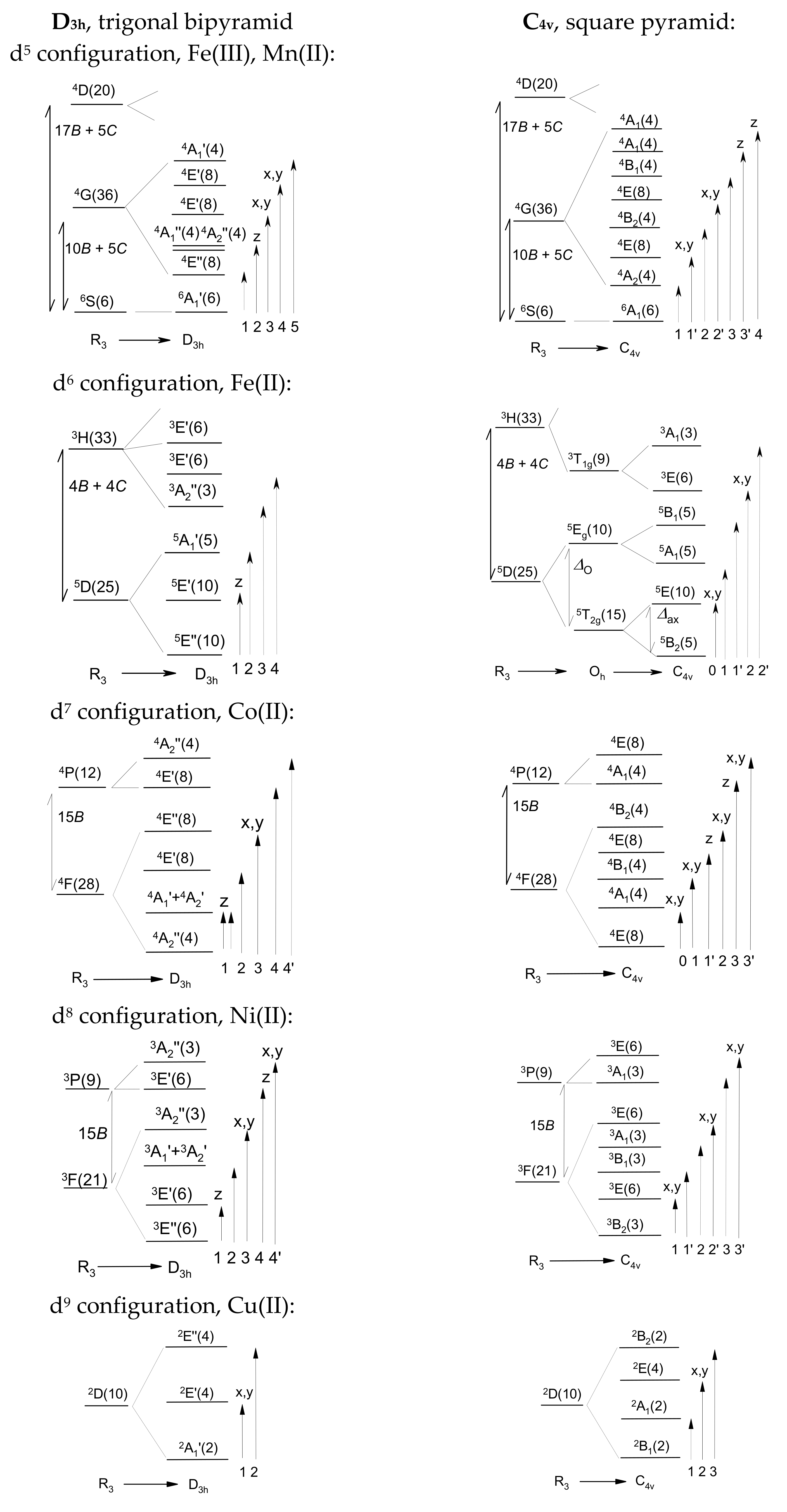
Figure 1 displays the relative energies of the crystal field terms (not to scale) for individual dⁿ configurations. These result from the GCFT calculations using the weak crystal field characterized by the crystal field poles F₄(L) = 5000 cm⁻¹ for each ligand. For the tetragonal pyramid (C_4v), the angle L^a-M-L^e = 104 deg was maintained. The passage from the fully rotation group R₃ of a free atom to point group D_3h or C_4v is shown as the splitting of the atomic terms by the crystal field. The literature outlines the branching rules for such a reduction process [9].

The character tables for the point groups usually assign the dipole moment components to the IRs; these are useful in determining the selection rules for the excitation energies. For instance, within group D_3h, the direct product of IRs is ${\mathrm{A}}_1^{\prime }\otimes {\mathrm{A}}_2^{″}={\mathrm{A}}_2^{″}\in z$, meaning that the z component of the dipole moment is active in transition ${\mathrm{A}}_1^{\prime }\to {\mathrm{A}}_2^{″}$, yielding the non-zero transition moment $〈{\mathrm{A}}_1^{\prime }\left|{\mu }_z\right|{\mathrm{A}}_2^{″}〉\ne 0$ (orbitally allowed transition). On the contrary, ${\mathrm{A}}_1^{\prime }\otimes {\mathrm{A}}_1^{″}={\mathrm{A}}_1^{″}\notin x,y,z$ and thus transition $〈{\mathrm{A}}_1^{\prime }\left|{\mu }_{x,y,z}\right|{\mathrm{A}}_1^{″}〉=0$ are forbidden.

In addition to the energy levels, Figure 1 also shows the allowed/forbidden polarized electronic dipole transitions, which are displayed as solid/dashed arrows. These data can be compared with the observations of the electronic d-d spectra [10].

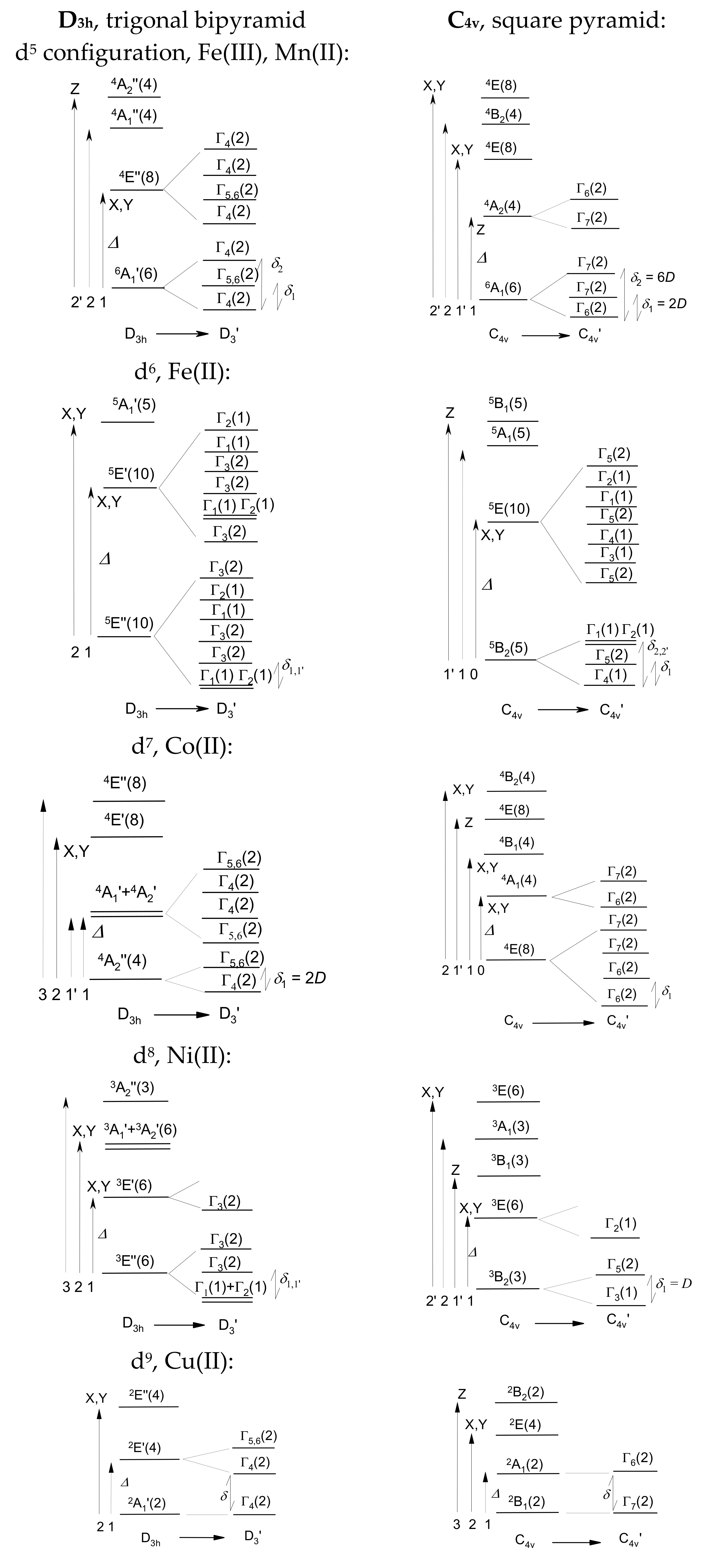
2.2. Crystal Field Multiplets

The crystal field terms represent a starting point for the further precision of the energy levels: upon introduction of the spin–orbit interaction, the crystal field terms are further spit into a set of crystal field multiplets (energy levels in the zero magnetic field) [11,12]. The basis set and the resulting multiplets contain 256, 210, 120, 45 and 10 members for electron configurations d⁵ through d⁹, respectively. In this case, the energy levels are labelled using the Bethe notation for the IRs within double group G’. These symbols involve Γ₁ through Γ₈, and their degeneracy is shown parentheses, e.g., Γ₄(2). (The IR tables for the double groups are useful for practical reasons).

The spin and the orbital parts of the wave function are assessed independently. For instance, in D_3h the level, ⁶A_1′(6) transforms its spin according to {2Γ₄ + (Γ₅ + Γ₆)}. The orbital part matches A₁ = Γ₁. Finally, the spin–orbit wavefunction transforms according to the direct product {2Γ₄ + (Γ₅ + Γ₆)}$\otimes$Γ₁, and the result is {2Γ₄ + (Γ₅ + Γ₆)}. In this special case, the levels (Γ₅ + Γ₆) form a complex conjugate pair that can be abbreviated as Γ_5,6(2) or simply Γ₅(2). To this end, upon passage from the D_3h to double group D’₃, the crystal field term ⁶A_1′(6) is split into a set of {2Γ₄(2) + Γ_5,6(2)} multiplets. However, this part of the theory says nothing about the relative energies of the final three Kramers doublets; these result from numerical calculations by GCFT.

The principal result of the CGTF calculations with spin–orbit coupling in the complete space spanned by dⁿ configurations is the spectrum of the crystal field multiplets. The lowest zero-field energy gaps are abbreviated as δ₁, δ₂, …, provided that the energy of the ground multiplet (δ₀) is set to zero (

Table 1. Multiplet gaps (in cm−1) calculated by GCFT for pentacoordinate systems.

System	D3h, Trigonal Bipyramid	C4v, Square Pyramid
Fe(III), F4 = 15,000 cm−1	6A1′: δ1(2) = 3.68 (4D), δ2(2) = 5.53 (6D)	6A1: δ1(2) = 1.50 (2D), δ2(2) = 4.51 (6D)
Fe(III), F4 = 5000 cm−1	6A1′: δ1(2) = 0.29 (4D), δ2(2) = 0.44 (6D)	6A1: δ1(2) = 0.10 (2D), δ2(2) = 0.31 (6D)
Fe(II), F4 = 5000 cm−1	5E″: δ1(2) = 85, δ2(2) = 180, δ3,3′(2) = {270, 301}, δ4(2) = 400	5B2: δ1(2) = 0.31 (D), δ2,2′(2) = {1.64, 1.87} (~4D)
Co(II), F4 = 5000 cm−1	4A2″: δ1(2) = 84.7 (2D)	4E: δ1(2) = 220, δ2(2) = 389, δ3(2) = 697
Ni(II), F4 = 5000 cm−1	3E″: δ1(2) = 533, δ2(2) = 1191	3B2: δ1(2) = 27.4 (D)
Cu(II), F4 = 5000 cm−1	2A1: Δ = 3020	2B1: Δ = 1691

). For the non-degenerate ground state (A or B type), the lowest multiplet gaps relate to the axial zero-field splitting parameter (D). For d⁵-Fe(II) (and, analogously, d⁵-Mn(III)), the sequence of the spin–orbit multiplet does not strictly follow D and 4D (there is a small difference (δ_a) around 4D). For Cu(II), the ground electronic term is not split by the spin–orbit interaction; however, the spin–orbit multiplets are slightly influenced by the spin–orbit coupling. The concept of the D parameter is strictly related to the spin–Hamiltonian theory.

The effect of the spin-orbit interaction leading to the passage from the crystal-field terms to the crystal-field multiplets is depicted in Figure 2.

2.3. Zero-Field Splitting

The concept of the spin Hamiltonian is a popular and very useful tool for interpretation of the spectra of electron paramagnetic resonance, as well as for analysis of DC magnetometric data. The key formulae of the spin Hamiltonian are based on consideration of only the spin kets $\left|S,M_S\right.〉$ of non-degenerate ground term A or B. The second-order perturbation theory offers the Λ tensor in the following form:

$${\Lambda }_{ab}=-{\hslash }^{-2}{\displaystyle \sum _{K\ne 0}\frac{〈0\left|{\widehat{L}}_a\right|K〉〈K\left|{\widehat{L}}_b\right|0〉}{E_K-E_0}}$$

(5)

where K runs over all excited electronic terms, and the magnetic tensors are expressed as follows:

• the κ tensor (reduced, temperature−independent paramagnetic susceptibility tensor):

  $${\kappa }_{ab}^{\mathrm{para}}={\mu }_{\mathrm{B}}^2{\Lambda }_{ab}$$

  (6)
• the g tensor (magnetogyric ratio tensor):

  $$g_{ab}=g_{\mathrm{e}}{\delta }_{ab}+2\lambda {\Lambda }_{ab}$$

  (7)
• the D tensor (spin–spin interaction tensor):

  $$D_{ab}={\lambda }^2{\Lambda }_{ab}$$

  (8)

This approximation fails in the case of orbital (pseudo) degeneracy. The matrix elements of the angular momentum $〈0\left|{\widehat{L}}_a\right|K〉$ can be assessed by exploiting the symmetry of the ground and excited crystal field terms; the matrix element is non-zero only if the direct product (${\mathsf{\Gamma }}_0\otimes {\mathsf{\Gamma }}_K={\mathsf{\Gamma }}_{Lx,Ly,Lz}+\dots$) contains the irreducible representation of at least one component of the angular momentum. For instance, within group D_3h, ${\mathrm{A}}_1^{\prime }\otimes {\mathrm{E}}^{″}={\mathrm{E}}^{″}\in L_{x,y}$ and the common character tables indicate that the result contains the irreducible representation of L_x and L_y.

The spin Hamiltonian parameters calculated via the GCFT are listed in

Table 2. Calculated spin Hamiltonian parameters for pentacoordinate systems.

Center	D3h, Trigonal Bipyramid			C4v, Square Pyramid
	D/hc/cm−1	gz, gxy	χTIP/10−9 [SI] 1	D/hc/cm−1	gz, gxy	χTIP/10−9 [SI] 1
Fe(II)	undefined	2.002, 2.096	2.05	0.50	2.111, 2.121	3.77
Co(II)	42.8	2.002, 2.500	6.34	undefined	2.218, 2.494	7.62
Ni(II)	undefined	2.002, 2.401	2.77	36.6	2.343, 2.576	5.16
Cu(II)	undefined	2.002, 2.672	1.76	undefined	2.901, 2.294	1.95

¹ SI unit for χ_TIP is m³ mol⁻¹. Calculated according to the weak-field limit of F₄ = 5000 cm⁻¹.

. For Fe(III) and Mn(II), the ground electronic term ⁶A does not allow transitions to excited terms with different spin multiplicities. Therefore, D = 0, g_i = g_e in this approximation. In this case, the spin Hamiltonian formalism is insufficient, so ⁶A₁ + ⁴T₁ terms must be considered for the O_h symmetry [13].

The spin Hamiltonian is often presented in the following form:

$${\widehat{H}}^{\mathrm{zfs}}=[D({\widehat{S}}_z^2-{\widehat{S}}^2/3)+E({\widehat{S}}_x^2-{\widehat{S}}_y^2)]{\hslash }^{-2}$$

(9)

where the D tensor is considered diagonal and traceless, yielding only two independent parameters: the axial zero-field splitting parameter (D) and the rhombic zero-field splitting parameter (E). This form is widely used for analysis of magnetometric and EPR data. According to convention, the rhombic part is minor: |D| > 3E > 0. D serves as a measure of zero-field splitting. This energy gap can also be measured also by FAR-infrared spectroscopy (FIRMS and FDMRS techniques), inelastic neutron scattering, calorimetry, etc. [14].

As mentioned above, the case of d⁶-Fe(II) or d⁶-Mn(III) is specific, as for C_4v geometry, the sequence of the spin–orbit multiplets differs depending on the exact multiplet splitting {0, δ₁(2), δ_22′(1 + 1) and the spin Hamiltonian formalism {0, D(2), 4D(2)}; the number in parentheses corresponds to the multiplicity. The ground crystal field term is ⁵B₂; the orbital and spin parts transform as B₂ → Γ₄, S = 2 → Γ₁ + Γ₃ + Γ₄ + Γ₅, and their direct product is Γ₄$\otimes$(Γ₁ + Γ₃ + Γ₄ + Γ₅) = Γ₁(1) + Γ₂(1) + Γ₄(1) + Γ₅(2). Only Γ₅(2) is doubly degenerate, whereas the remaining multiplets are nondegenerate: Γ₁(1), Γ₂(1), and Γ₄(1). The GCFT calculations for d⁶-Fe(II) in the complete basis set of 210 kets obtains Γ₄ as the ground multiplet and the multiplet splitting E(Γ₅) − E(Γ₄) = δ₁ = 0.31 cm⁻¹; E(Γ₁) − E(Γ₄) = δ₂ = 1.64 cm⁻¹; E(Γ₂) − E(Γ₄) = δ_2′ = 1.87 cm⁻¹. This feature is reflected in the spectrum of electron paramagnetic resonance. Details about the symmetry rules are listed in Supplementary Information.

Table 3. Review of the SH formalism for pentacoordinate systems ¹.

System	D3h, Trigonal Bipyramid τ5 = 1	C2v, Intermediate Geometry τ5 = 0.47	C4v, Square Pyramid τ5 = 0
d1, Ti(III)	2E″, D—undefined	2A2, D—undefined	2B2, D—undefined
d2, V(III)	3A2″, D = 16	3B1, D = 19, E = 0.3	3E, D—undefined
d3, Cr(III)	4E″, D—undefined	4A2, 2D = −17, E = 0.6	4B2, 2D = 6.2
d4, Mn(III)	5A1′, D = 3.2	5A1, D = 3.1, E = 0.4	5B1, D = −2.9
d5, Fe(III)	6A1′, D—small	6A1, D—small	6A1, D—small
d6, Fe(II)	5E″, D—undefined	5A2, D = −8, E = 1	5B2, D = 0.5
d7, Co(II)	4A2″, 2D = 85	4B1, 2D = 102, E = 1	4E, D—undefined
d8, Ni(II)	3E″, D—undefined	3A2, D = −105, E = 7	3B2, D = 37
d9, Cu(II)	2A1′, D—undefined	2A1, D—undefined	2B1, D—undefined

¹ The Addison structural parameter (τ₅ = (β − α)/60), where: β > α are the two greatest valence angles of the coordination center [15]. Data on D and E in cm⁻¹ calculated with F₄ = 5000 cm⁻¹.

shows a comparison of the dⁿ configurations from the viewpoint of the spin Hamiltonian formalism. This table is also enriched by data for d¹ to d⁴ configurations, as well as data for the intermediate geometry with C_2v symmetry and τ₅ = 0.47.

Table 4. Review of the SH formalism for hexacoordinate systems with tetragonal distortion ¹.

System	D4h, Compressed Bipyramid	Oh, Octahedron	D4h, Elongated Bipyramid
d1, Ti(III)	2Eg, D—undefined	2T2g, D—undefined	2B2g, D—undefined
d2, V(III)	3A2g, D = 55	3T1g, D—undefined	3Eg, D—undefined
d3, Cr(III)	4B1g, 2D = −0.7	4A2g, D = 0	4B1g, 2D = 0.9
d4, Mn(III)	5A1g, D = 2.5	5Eg(JT), D—undefined	5B1g, D = −2.8
d5, Fe(III)	6A1g, D—small	6A1g, D—small	6A1g, D—small
d6, Fe(II)	5Eg, D—undefined	5T2g, D—undefined	5B2g, D = 16
d7, Co(II)	4A2g, 2D = 300	4T1g, D—undefined	4Eg, D—undefined
d8, Ni(II)	3B1g, D = −4.3	3A2g, D = 0	3B1g, D = 5.3
d9, Cu(II)	2A1g, D—undefined	2Eg(JT), D—undefined	2B1g, D—undefined

¹ JT points to a strong Jahn–Teller effect, owing to which a spontaneous symmetry descent proceeds. Data on D in cm⁻¹ calculated with F₄ = 5000 cm⁻¹.

analogously summarizes data for the hexacoordinate complexes.

2.4. DC Magnetic Functions

The magnetic energy levels ${\epsilon }_{i,a}(B_m)$ result from the diagonalization of the interaction matrix ((a) + (b) + (c) + (d) + (e)), which includes interelectronic repulsion, crystal field potential, spin–orbit coupling, and orbital and Zeeman terms in the applied magnetic field. Statistical thermodynamics offers formulae for magnetization and magnetic susceptibility when the partition function is evaluated for three reference fields: B_m = B₀ − δ, B₀, B₀ + δ (allowing numerical derivatives):

$$Z_a(T,B_m)={\displaystyle \sum _i\exp [{\epsilon }_{i,a}(B_m)/k_{\mathrm{B}}T]}$$

(10)

Hence, the molar magnetization is:

$${(M_{\mathrm{mol}})}_a=\frac{RT}{Z_a}{\left(\frac{\partial Z_a}{\partial B_a}\right)}_T$$

(11)

The molar magnetic susceptibility is expressed as:

$${({\chi }_{\mathrm{mol}})}_{ab}={\mu }_0{\left(\frac{\partial {(M_{\mathrm{mol}})}_a}{\partial B_b}\right)}_T$$

(12)

where the physical constants adopt their usual meaning. The index a refers either to the Cartesian coordinates {x, y, z} or to the grid point over a sphere along which the magnetic field is aligned, which is used to obtain the powder-sample average. Therefore, the magnetic susceptibility and magnetization are functions of discrete parameters (atomic parameters B_M, C_M, and ξ_M; ligand positions θ_L and φ_L; crystal field poles F₄(L); and eventually F₂(L)), as well as the continuous parameters, such as the reference field (B_m) and temperature (T).

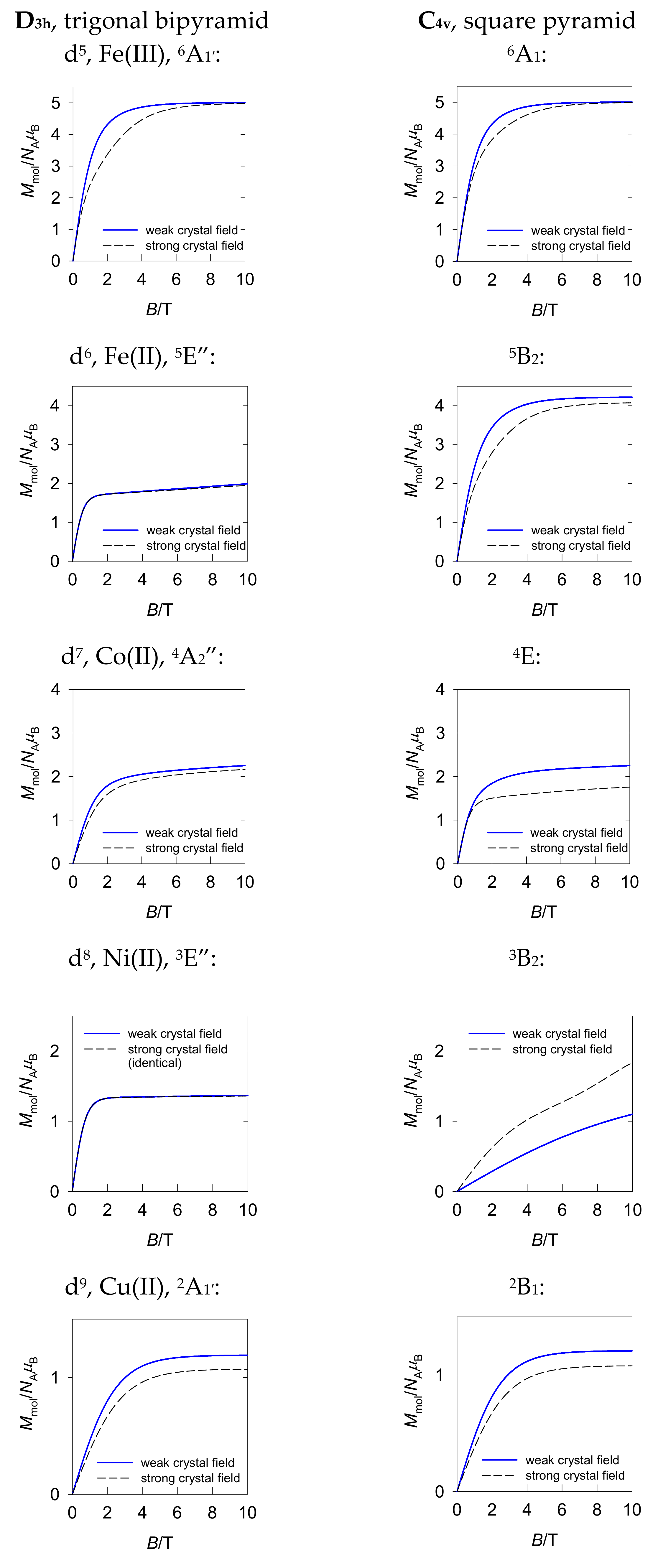
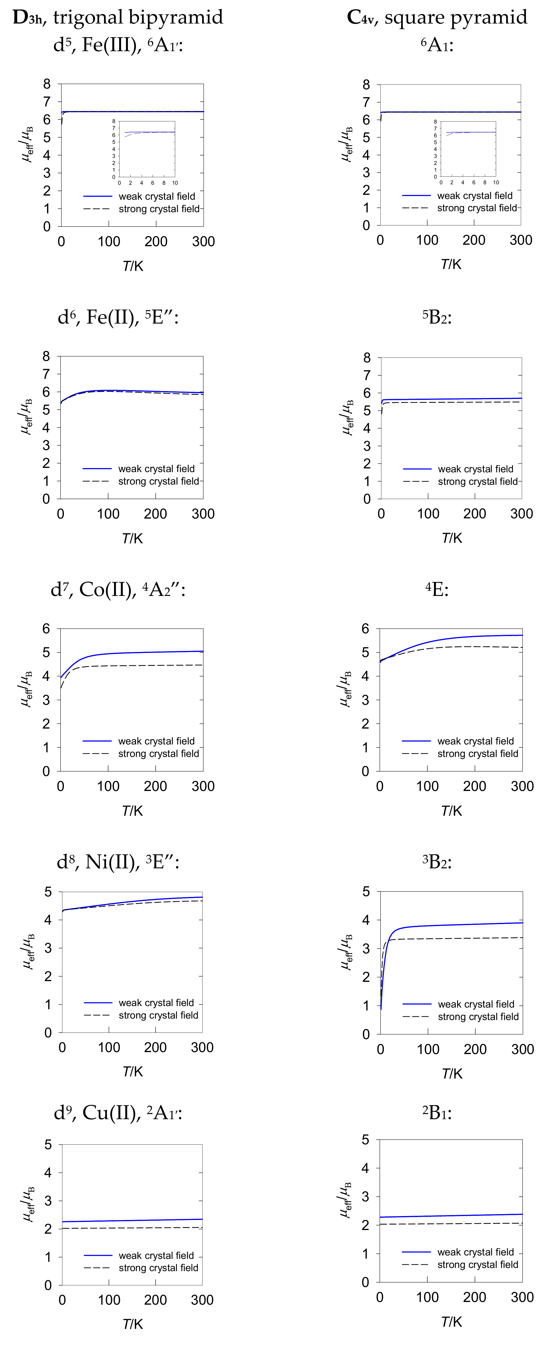
The modelling of the magnetization and susceptibility for pentacoordinate dⁿ systems is presented in Figure 3 and Figure 4. A counterpart of these graphs for the tetragonally distorted octahedral systems can be found elsewhere [16]. In the case of zero-field splitting with an orbitally non-degenerate ground term, the effective magnetic moment in the high-temperature limit of 300 K remains almost linear with zero slope; at low temperature, it is reduced. This is the case of d⁵-D_3h, d⁵-C_4v, d⁶-C_4v, d⁷-D_3h, and d⁸-C_4v. For d⁹-D_3h and d⁹-C_4v, zero-field splitting is absent, so these systems follow the Curie law. The magnetization saturates to the value of M₁ = M_mol/(N_Aμ_B) = g_avS when the zero-field splitting is small. This is the case of d⁵-D_3h, d⁵-C_4v, d⁶-C_4v, d⁹-D_3h, and d⁹-C_4v; exceptions are d⁷-D_3h and d⁸-C_4v, with large zero-field splitting D parameters.

Systems with E-type orbitally doubly degenerate ground terms, such as d⁶-D_3h, d⁷-C_4v, and d⁸-D_3h behave differently. The effective magnetic moment is enlarged, and it passes through a round maximum. The magnetization is also suppressed and does not reach saturation until B = 10 T.

A positive slope of the effective magnetic moment reflects the effect of the low-lying excited electronic terms mixed considerably with the ground term via the spin–orbit interaction. This results in temperature-independent paramagnetism, χ_TIP > 0. This term, along with the underlying diamagnetism (χ_dia < 0), need be subtracted from the measured temperature dependence of the magnetic susceptibility. With respect to the underlying diamagnetism, a method of additive Pascal constants is useful and frequently utilized. However, for temperature-independent paramagnetism, the amount of information is considerably limited [6,7].

2.5. AC Magnetic Susceptibility

In the oscillating magnetic fields (usually with a low amplitude of B_AC = 0.3 mT and a frequency range of f = 10⁻²–10⁵ Hz), the measured magnetic moment of the specimen has two components: in-phase and out-of-phase. This is easily transformed into two components of AC susceptibility: χ′ (dispersion) and χ″ (absorption). The absorption component is a measure of the resistivity of the sample used to alter its magnetization; it provides information about the relaxation time, which is a function of temperature, frequency (f), and the external applied field (B_DC). The relaxation time can be inferred from the position of the maximum at the out-of-phase susceptibility (f″_max) with the following formula: τ = 1/(2πf″_max). It has been reported that the sample can exhibit two or more relaxation channels and that their absorption curves can overlap or merge to form a shoulder. The whole AC susceptibility can be fitted by exploiting the generalized Debye equation [17,18]:

$$\chi (\omega )={\chi }_S+{\displaystyle \sum _k^K\frac{{\chi }_k-{\chi }_{k-1}}{1+(\mathrm{i}\omega {\tau }_k{)}^{1-{\alpha }_k}}}$$

(13)

where K is the number of relaxation channels, χ_S is the common adiabatic susceptibility (high-frequency limit), χ_k is the thermal susceptibilities, α_k is the distribution parameters, τ_k is the relaxation times, and the circular frequency is ω = 2πf. This complex equation can be decomposed into a real and imaginary part.

The slow magnetic relaxation includes several mechanisms that can be collected to a single equation for the reciprocal relaxation time:

$${\tau }^{-1}={\tau }_0^{-1}\exp \left(-U_{\mathrm{eff}}/k_{\mathrm{B}}T\right)+C_{\mathrm{R}}{T}^n+C_{\mathrm{pb}}{T}^l+A{B}^{m}T+D_1/(D_2+B^2)$$

(14)

The first term describes the thermally activated Orbach process, which is associated with the height of the barrier to spin reversal (U_eff); the second is the Raman term, with the temperature exponent typically n = 5–9; next is the phonon bottleneck term, with l ~ 2; the fourth term describes the direct relaxation process, with m = 2–4; the last term refers to the quantum tunnelling of magnetization throughout the barrier to spin reversal. The reciprocating thermal behavior was recently registered with a term analogous to the phonon bottleneck but a negative temperature exponent (l ~ −1) [18].

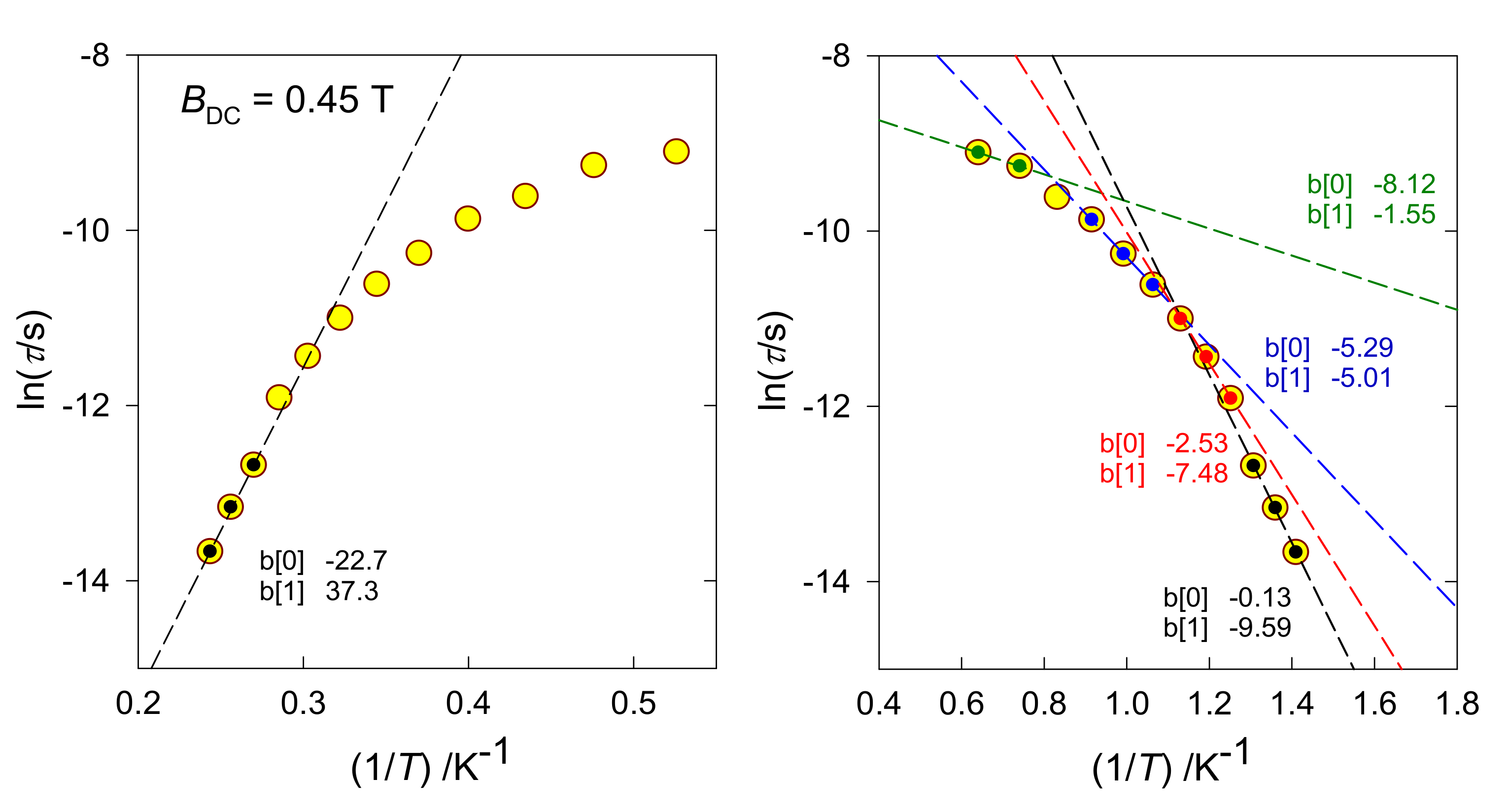
The effectiveness of the slow magnetic relaxation is, as a rule, evaluated by the value of U_eff (when the Orbach process applies). It is assumed that it is related to the axial zero-field splitting parameter (D), which must be negative, and the molecular spin (S) [19]:

$$U_{\mathrm{eff}}=\left|D\right|(S^2-1/4),$$

(15)

which holds true for Kramers systems with half-integral spin (e.g., S = 3/2 for Co^II); for non-Kramers systems with an integer spin, the factor ¼ is dropped (e.g., S = 1, for Ni^II). It is common practice for the U_eff and the pre-exponential factor (τ₀) to be subtracted using the Arrhenius-like plot ln(τ) vs. 1/T (Figure 5-left): a few high-temperature points are fitted by the straight line, tangential of which refers to U_eff. However, “high-temperature points” refer to the highest temperature among the data considered in our analysis, so there still could be points yielding a higher tangential and thus U_eff. A preferred approach involves plotting ln(τ) vs. ln(T), where the temperature exponent recovering the high-temperature data refers to the slope (Figure 5, right). When the temperature coefficient is n > 9, instead of the Raman process the Orbach process is applied.

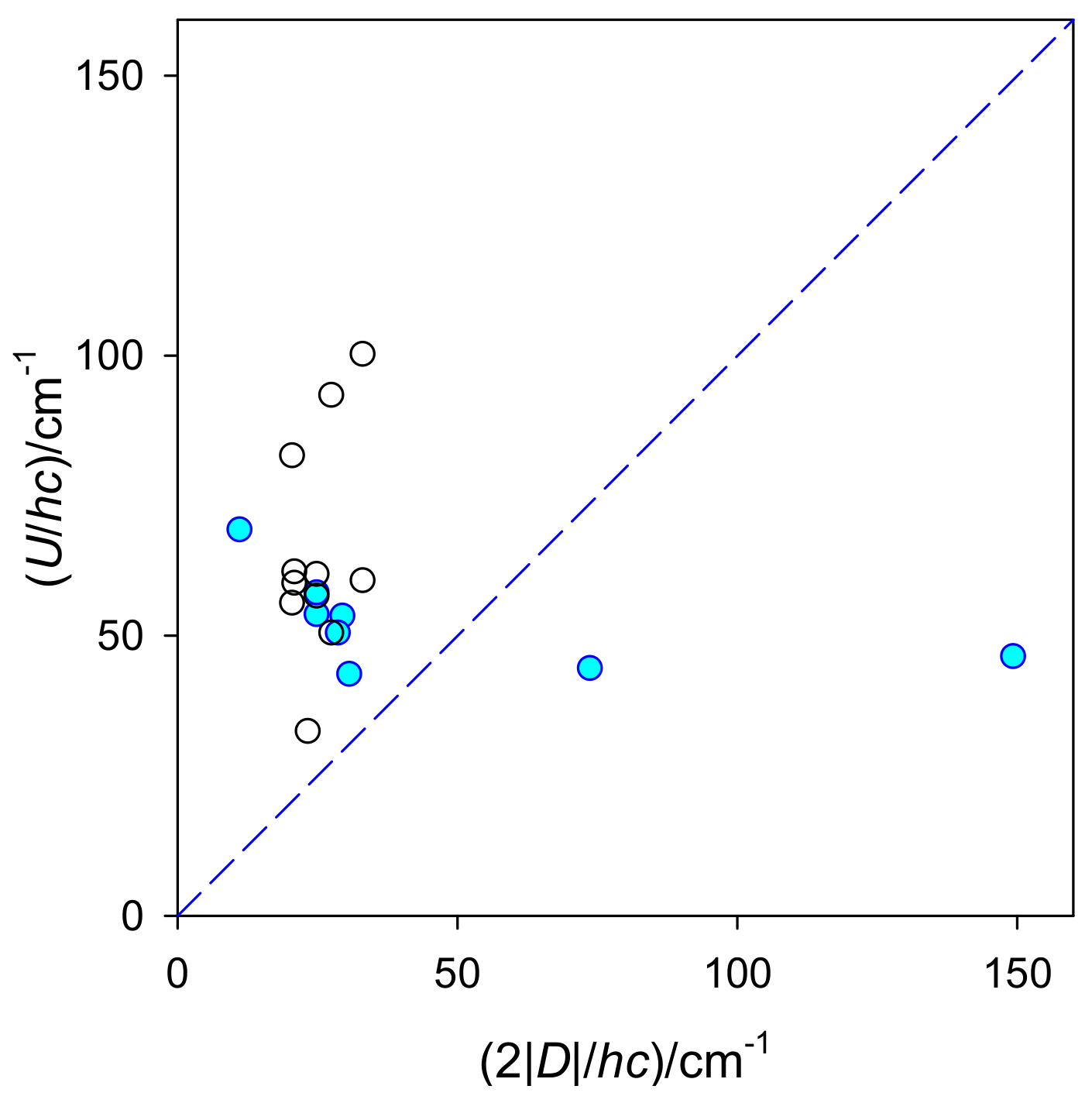
For high-spin Co(II) complexes with S = 3/2, eqn (15) implies a relationship of U = 2|D|. A collection of experimental data for a series of tetracoordinate Co^II complexes is shown in Figure 6 based on the analysis of higher-temperature, high-frequency relaxation data in terms of the Orbach process. Evidently, a correlation of U vs. 2|D| fails. D is a field-independent quantity, whereas the extracted value of U depends upon the applied magnetic field. A positive value of D contradicts the D-U paradigm; however, SIMs behavior can occur (the Raman mechanism is likely the leading term). With increased barrier to spin reversal (U), the extrapolated relaxation time (τ₀) is shortened, irrespective of the sign of the D parameter. A violation of the D-U paradigm has been discussed elsewhere with consideration of anharmonicity contributions [21].

3. Discussion

The GCFT approach enables fast and “continuous” mapping of the energy levels, such as electronic terms and the spin–orbit multiplets: one is free to changing the ligand positions {θ_L, φ_L} from regular coordination polyhedra to distorted polyhedra and to alter the crystal field poles F₄(L) and, eventually, F₂(L). On the contrary, the modern ab initio calculations provide high-quality data on energy levels but only for the unique geometry of the complex under investigation. Therefore, it is interesting to utilize and compare both approaches.

Ab initio calculations have been performed using ORCA software [22] with respect to the experimental geometry of the complexes resulting from X-ray structural analysis (the corresponding cif files are deposited in the Cambridge Crystallographic Data Centre). The relativistic effects were included in the calculations with a second-order Douglas–Kroll–Hess (DKH) procedure. An extended basis set TZVP of Gaussian functions was used, e.g., BS1 = [17s11p7d1f] and BS2 = [17s12p7d2f1g] for Ni(II). The calculations were based on state-average complete active-space self-consistent field (SA-CASSCF) wave functions. The active space of the CASSCF calculations comprised eight electrons in five metal-based d-orbitals. The state-averaged approach was used, whereby all 10 triplet and 15 singlet states were equally weighted. The spin–orbit effects were included according to quasi-degenerate perturbation theory, whereby the spin–orbit coupling operator (SOMF) was approximated according to the Breit–Pauli form. The electronic terms were evaluated at the CASSCF + NEVPT2 level, and the multiplets by considering the spin–orbit interaction (

Table 5. Energy levels for representative Ni(II) complexes calculated by ab initio method 1.

System	Donor Set, Symmetry	SHAPE Index	Reported D/cm−1	Δ/cm−1 NEVPT2	δ/cm−1 SOC	D/cm−1 E/D
[Ni(Me4cyclam)N3]ClO4	NiN4N′ C2v	vOC-5: 0.61 SPY-5: 0.72	+20, mag +21, EPR	a3A: 0, b3A: 5777	a3A → 0, 23, 27	25 0.08
[Ni(iPrtacn)Cl2]	NiN3Cl2 τ5 = 0.42	vOC-5: 2.91 SPY-5: 3.53	+14.3, mag +15.7, EPR +15.9, FDMRS	a3A: 0, b3A: 5815	a3A → 0, 17, 24	20 0.18
[Ni(iPrtacn)Br2]	NiN3Br2 τ5 = 0.40	vOC-5: 2.83 SPY-5: 3.72	+11.0, mag +13.9, EPR +13.8, FDMRS	a3A: 0, b3A: 6035	a3A → 0, 13, 21	17 0.21
[Ni(iPrtacn)(NCS)2]	NiN3N′2 τ5 = 0.44	vOC-5: 2.56 SPY-5: 2.72	+13.8, mag +16.1, EPR +15.9, FDMRS	a3A: 0, b3A: 5846	a3A → 0, 15, 27	25 0.28
[Ni(Me6tren)Cl]ClO4	NiN3N′Cl C3v	TBPY-5: 0.61	−179, EPR −110, FIRMS −205, calc	a3E: 0, 26, b3E: 5775, 5782	a3E → 0, 5, 512, 538, 1162, 1162	-
[Ni(Me6tren)Br]Br	NiN3N′Br C3v	TBPY-5: 0.92	−147, calc	a3E: 0, 5 b3E: 7100,7106	a3E → 0, 3, 545, 550, 1196, 1196	-
[Ni(MDABCO)2Cl3]ClO4	NiCl3N2, D3h, τ5 = 1	TBPY-5: 0.14	−311, mag −535, EPR	a3E: 0, 342, b3E: 6517, 6874	a3E → 0, 0.3, 397, 735, 1243,1252	-

¹ Abbreviations: mag—magnetometry, EPR—(high-field/high-frequency) electron paramagnetic resonance, FDMRS—frequency-domain magnetic resonance spectroscopy, FIRMS—far infrared magnetic spectroscopy; SHAPE index (consistency with the regular coordination polyhedron) [23]: TBPY—trigonal bipyramid, SPY—square pyramid, vOC—vacant octahedron; electronic terms a³A—ground-spin triplet, b³A—first excited spin triplet, a³E—ground-orbital doublet, b³E—first excited orbital doublet; ground spin–orbit multiplet at zero; δ—separation of the lowest multiplets: three from term a³A (consistent with the spin Hamiltonian formalism), six from a³E (beyond the spin Hamiltonian formalism). Structural and experimental data according to Refs. [24,25,26,27,28]. Ab initio calculations were carried out according to the same protocol.

). Effective Hamiltonian was used to evaluate the spin Hamiltonian parameters.

The ab initio calculations refer to in silico state, i.e., intermolecular interactions and other solid-state effects are ignored. This is not the case for experimental magnetometric or spectroscopic data, which could be influenced by the environment. The ab initio data, in general, are consistent with those obtained by experimental techniques.

When comparing the CGTF calculations with ab initio calculations, calculated transition energies can be assessed. With a proper set of crystal field poles, the CGTF can reproduce first allowed transitions; however, the electronic spectrum, has a smaller width with respect to ab initio data.

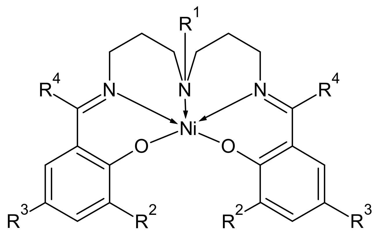
An extended set of similar pentacoordinate Ni(II) complexes based on the fixed skeleton of a pentadentate Schiff base (Figure 7) was investigated by magnetometry and ab initio calculations with respect to the experimental geometry; these are listed in

Table 6. Magnetometric and ab initio data for a set of pentadentate Ni(II) complexes comprising Schiff base ligands ¹.

System	Addison Index τ5	SHAPE Index	D/cm−1 Magnetometry	δ/cm−1 SOC	D/cm−1 Calculations	E/D
1	0.52	TBPY-5: 1.583, SPY-5: 1.664	−45.1	0, 4, 51	−49.1	0.045
2	0.62	TBPY-5: 0.899, SPY-5: 2.589	−64.0	0, 5, 55	−52.6	0.044
3	0.62	TBPY-5: 0.903, SPY-5: 2.598	−60.2	0, 5, 54	−52.0	0.047
4	0.47	vOC-5: 1.881, SPY-5: 1.508	−45.1	0, 6. 44	−41.7	0.068
5	0.60	TBPY-5: 1.050, SPY-5: 2.072	−49.3	0, 5, 66	−63.2	0.037
6	0.26	vOC-5: 0.909, SPY-5: 0.913	−12.7	0, 8, 30	−25.3	0.169

¹ Data from ref. [29].

.

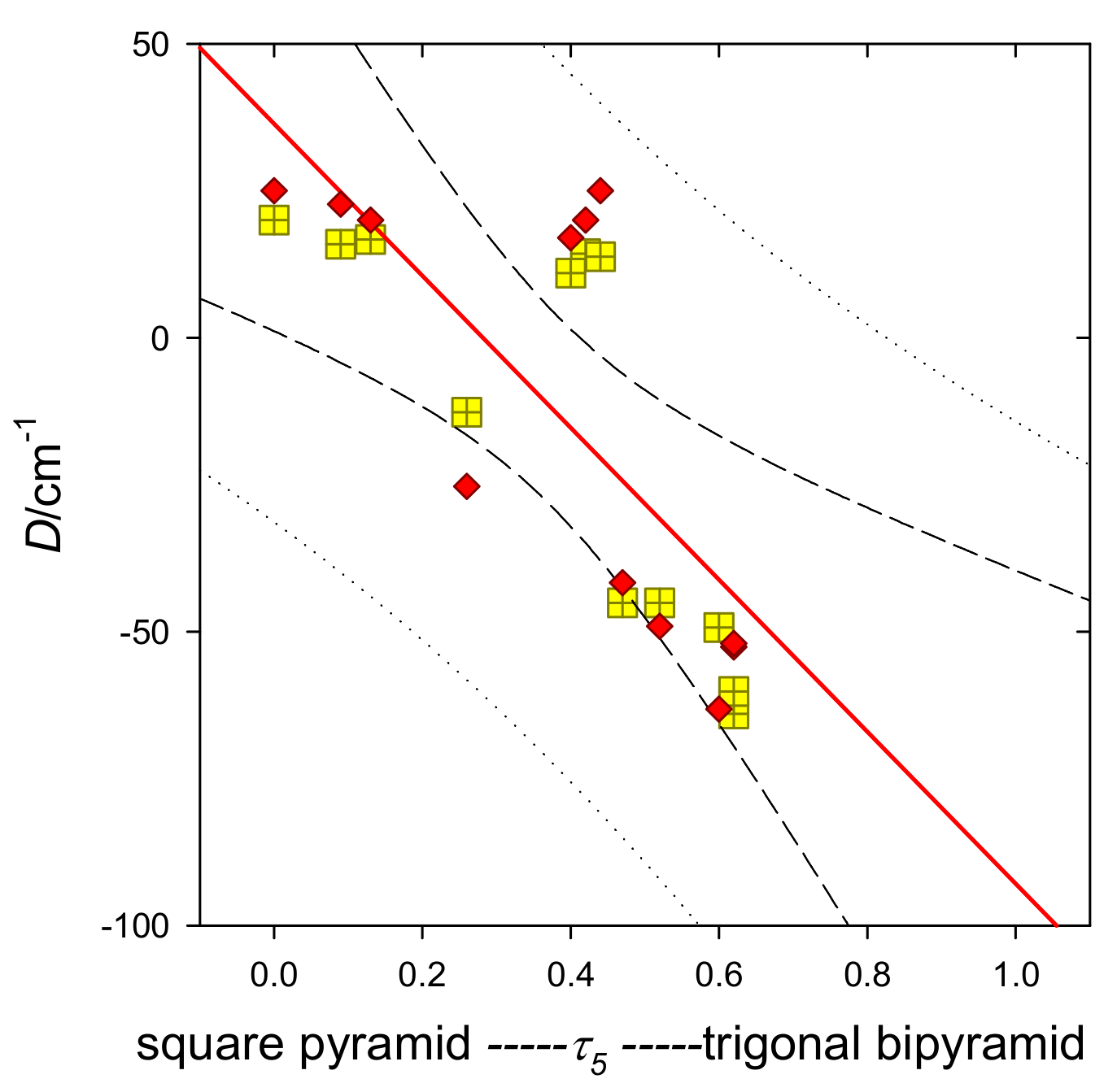
The experimentally reported and calculated D values cover a broad interval of positive and negative values over a wide range of the τ₅ parameters. These were used to plot D vs. τ₅, which can be termed the second magnetostructural D-correlation for Ni(II) complexes (MSDC). (The first magnetostructural D correlation for hexacoordinate Ni(II) complexes is outlined elsewhere [30].) The MSDC can be approximated by a straight line (Figure 8) when the τ₅ parameter guarantees that the ground electronic term is not orbitally quasi-degenerate (the energy gap Δ > 2000 cm⁻¹). In the opposite case, the calculated D values tend to diverge. The value of the D parameter switches between positive and negative values at τ₅ ~ 0.2–0.3. Furthermore, the E parameter plays a role that has not be considered so far.

4. Conclusions

Experimental data on magnetic susceptibility, magnetization, and electron paramagnetic resonance require an appropriate model in order be analyzed correctly. For some shapes of coordination polyhedra, such as octahedron O_h, tetragonal bipyramid D_4h, trigonal antiprism D_3d, tetrahedron T_d, and bispehoid D_2d, the crystal field theory offers such a support, and the spin Hamiltonian formalism defines relationships for the set of magnetic parameters (D, E, g_x, g_y, g_z, χ_TIP). A dearth in the literature with respect to pentacoordinate systems, such as the trigonal bipyramid D_3h and tetragonal pyramid C_4v symmetry, is filled by this publication. The working tool is the generalized crystal field theory in the form of its fully numerical, computer-assisted tool [31]. The advantage of this approach is that the positions of the ligands can be arbitrary, making it applicable to any geometry of the chromophore and any ligands. Only the set of Racah parameters of the interelectronic repulsion (B_M and C_M), the spin–orbit coupling constant (ξ_M), polar angles (or Cartesian coordinates) of each ligand {θ_L, φ_L}, the crystal field poles F₄(L) and, eventually, F₂(L) are required. This method enables evaluation of the energies of the multielectron crystal field terms, spin–orbit crystal field multiplets, and the magnetic energy levels at the applied magnetic field. Then, the magnetic susceptibility and magnetization can be evaluated as functions of the temperature field via derivatives of the partition function. The eigenvectors provide complete information about the symmetry and can be used to automatically label terms/multiplets.