Controlling Resonance Fluorescence Spectra and Photon Statistics in a Driven V-Type Quantum Emitter—Metal Nanoparticle Coupled Structure

Abstract

We study the resonant fluorescence emission spectrum and the intensity-intensity correlations of the emitted fluorescent field by a V-type quantum emitter (QE) which is located near a metal nanosphere. For the description of the studied phenomena, we use the density matrix equations methodology combined with electromagnetic calculations and obtain results for the profile of the resonant fluorescence spectrum and the second-order correlation functions associated with the fluorescent photons. The decay rates and the coupling term exhibit a strong dependence on the distance that separates the QE from the metal nanoparticle. This distance also influences the resonance fluorescence of the V-type QE. We find that, in the general case, the resonant fluorescence spectrum is composed of five Lorentzian-type peaks, for high interparticle distances, while, when the QE is located very close to the surface of the nanosphere, the central resonance becomes dominant, and a single-peaked spectral profile appears. The two-time correlation functions of the fluorescent photons evolve in an oscillatory manner around unity, for non-zero time delay, with a period that decreases with the increase of the field intensity. In the strong driving field regime, the antibunching to bunching crossing time does not depend on the interparticle distance, contrary to the results found in the weak driving field regime. We also find that, for a weak laser field and under specific conditions, the second-order correlation functions constantly remain in the antibunching region.

1. Introduction

For over a decade, a problem that has attracted considerable attention in quantum photonics is the behavior of the resonance fluorescence spectrum of quantum emitters (QEs), like molecules and semiconductor quantum dots which are coupled with plasmonic nanostructures [1]. In this case, the presence of the plasmonic nanostructure near the QEs can strongly modify the shape of the resonance fluorescence spectrum emitted by the QEs, the width of the spectral resonances, as well as the photon statistics mainly analyzed by the fluorescent field intensity-intensity correlation functions [1,2,3,4,5,6,7,8,9,10,11,12,13,14,15,16,17,18,19,20,21,22,23,24]. These effects occur mainly due to of the dramatic change of the QE spontaneous decay rate near the plasmonic nanostructure due to the Purcell effect and due to the exciton-plasmon coupling.

The common energy level structure used for the QE is a single two-level system [1,2,3,4,5,6,7,8,9,10,11,12,13,14,15,16], while different structures have been considered like, for example, a couple of two-level quantum systems [17,18], as well as multi-level quantum systems including the cascade three-level structure [19,20], the Λ-type three-level structure [21], the V-type three-level structure [22] and double-Λ-quantum system [23], and the double-V-type four-level system [24]. The most common plasmonic nanostructure considered in these studies is a spherical metal nanoparticle [1,2,3,4,6,7,8,10,11,13,14,16,17,20,21,23], while more complex plasmonic nanostructures, like, for example, periodic metal-dielectric nanostructures [15,22,24], have been considered in different studies. An interesting phenomenon that appears in the V-type [22] and the double-V-type quantum systems [24] is the quantum interference in spontaneous emission due to the anisotropic Purcell effect [25,26,27,28,29,30,31,32,33,34], which can be also used for the modification of the resonance fluorescence spectrum and the intensity-intensity correlation function of the fluorescent photons.

In the present work, we study the resonant fluorescence emission spectrum and the two-time intensity correlations of the emitted fluorescent field by a V-type QE which is located near a metal nanosphere. For the description of the studied phenomena, we use the density matrix equations methodology combined with electromagnetic calculations and present results for the profile of the resonant fluorescence spectrum and the second-order correlation functions associated with the fluorescent photons. The decay rates and the coupling term exhibit a strong dependence on the distance between the QE and the metal nanoparticle. This distance also influences the resonance fluorescence of the V-type QE. We find that, in the general case, the resonant fluorescence spectrum is composed of five Lorentzian-type peaks, for high interparticle distances, while, for very close distances between the QE and the surface of the nanosphere, the central resonance becomes dominant, and a single-peaked spectral profile appears. The two-time correlation functions of the fluorescent photons evolve in an oscillatory manner around unity, with a period that decreases with the increase of the Rabi frequency. In the strong driving field regime, the antibunching to bunching crossing time does not depend on the interparticle distance, contrary to the results found in the weak driving field regime. We also find that, for a weak laser field and under specific conditions, the second-order correlation functions remain constantly in the antibunching region.

2. Methods

The hybrid system investigated in this work, which is presented in Figure 1a, is comprised of a QE described as a V-type energy-level scheme, as seen in Figure 1b, and a spherical gold nanoparticle with radius $R$ and dielectric function taken from experimental results [35]. In caption (a) of Figure 1, the blue arrows depict two alternative orientations of the transition dipole moment associated with the QE transitions, normal to and in parallel with the surface of the nanosphere. The corresponding distance is indicated by $d$. The laser field excites the $\left|0\right.〉\to \left|1\right.〉$, $\left|2\right.〉$ transitions. Its amplitude and angular frequency are denoted by $E_L$ and ${\omega }_L$, respectively. The electric dipole moments associated to the possible transitions are given by ${\overrightarrow{\mu }}_{01}=\frac{\mu }{\sqrt{2}}\left(\widehat{k}+i\widehat{i}\right)$, ${\overrightarrow{\mu }}_{02}=\frac{\mu }{\sqrt{2}}\left(\widehat{k}-i\widehat{i}\right)$, where $\widehat{i},\widehat{k}$ denote the unit vectors in the x and z directions, respectively and $\mu$ denotes the magnitude of the electric dipole moment [25,26,27,28,29,30,31,32,33,34]. In caption (b) of Figure 1, $\Delta$ is the detuning of the applied field from the resonance with reference to the $\left|0\right.〉\to \left|2\right.〉$ transition and $\hslash {\omega }_{21}$ is the energy difference between the excited levels $\left|1\right.〉$ and $\left|2\right.〉$. The decay rates of the transitions corresponding to the pathways $\left|n\right.〉\to \left|0\right.〉$, with $n=1,2$, are represented by ${\gamma }_n$, while the transition $\left|2\right.〉\to \left|1\right.〉$ is electric dipole-forbidden.

We denote by ${\Omega }_n=-{\mu }_n{E}_L/\hslash$ the Rabi frequency that corresponds to the $\left|0\right.〉\to \left|n\right.〉$ transition. With the electric field linearly polarized along the z axis, we take ${\Omega }_n=\Omega$, both for $n=1{,}_{}2$. The interaction of the QE with the coherent light field is described by the Hamiltonian operator, which is given by the following formula, in the dipole approximation:

$$H={\mathrm{E}}_1\left|1\right.〉\left.〈1\right|+{\mathrm{E}}_2\left|2\right.〉\left.〈2\right|+\hslash \Omega \left(\left|1\right.〉\left.〈0\right|+\left|2\right.〉\left.〈0\right|\right)e^{-i{\omega }_{L}t}+H.c.$$

(1)

where ${\mathrm{E}}_n$ is the energy of level $\left|n\right.〉$ (we consider that ${\mathrm{E}}_0=0$). Hence, based on the Liouville-von Neumann-Lindblad equation, we derive the following equations of motion that contain the density matrix elements, which, under the rotating wave approximation, are written as follows:

$$\begin{array}{l}{\dot{\rho }}_{10}(t)=-i(\Delta -{\omega }_{21}){\rho }_{10}(t)+\frac{i}{2}\Omega \left[{\rho }_{12}(t)+2{\rho }_{11}(t)+{\rho }_{22}(t)-1\right]\\ -\kappa {\rho }_{20}(t)-\gamma {\rho }_{10}(t),\end{array}$$

(2)

$${\dot{\rho }}_{20}(t)=-i\Delta {\rho }_{20}(t)+\frac{i}{2}\Omega \left[{\rho }_{21}(t)+2{\rho }_{22}(t)+{\rho }_{11}(t)-1\right]-\kappa {\rho }_{10}(t)-\gamma {\rho }_{20}(t),$$

(3)

$$\begin{array}{l}{\dot{\rho }}_{21}(t)=-i{\omega }_{21}{\rho }_{21}(t)+\frac{i}{2}\Omega \left[{\rho }_{20}(t)-{\rho }_{01}(t)\right]\\ -\kappa \left[{\rho }_{22}(t)+{\rho }_{11}(t)\right]-2\gamma {\rho }_{21}(t),\end{array}$$

(4)

$${\dot{\rho }}_{11}(t)=-\frac{i}{2}\Omega \left[{\rho }_{01}(t)-{\rho }_{10}(t)\right]-\kappa \left[{\rho }_{12}(t)+{\rho }_{21}(t)\right]-2\gamma {\rho }_{11}(t)\mathrm{and}$$

(5)

$${\dot{\rho }}_{22}(t)=-\frac{i}{2}\Omega \left[{\rho }_{02}(t)-{\rho }_{20}(t)\right]-\kappa \left[{\rho }_{12}(t)+{\rho }_{21}(t)\right]-2\gamma {\rho }_{22}(t)$$

(6)

Here, we have assumed that ${\gamma }_1={\gamma }_2=\gamma$ with

$$\gamma =\frac{({\Gamma }_{\perp }+{\Gamma }_{\parallel })}{2}$$

(7)

$$\kappa =\frac{({\Gamma }_{\perp }-{\Gamma }_{\parallel })}{2}$$

(8)

where the spontaneous emission rate for an electric dipole polarization oriented normal to $({\Gamma }_{\perp })$ and in parallel $({\Gamma }_{\parallel })$ with the surface of the nanosphere, are defined as ${\Gamma }_{\perp }={\mu }_0{\mu }^2{\overline{\omega }}^2\mathrm{Im}[G_{\perp }(\overrightarrow{r},\overrightarrow{r};\overline{\omega })]/\hslash$ and ${\Gamma }_{\parallel }={\mu }_0{\mu }^2{\overline{\omega }}^2\mathrm{Im}[G_{\parallel }(\overrightarrow{r},\overrightarrow{r};\overline{\omega })]/\hslash$, respectively, with ${\mu }_0$ denoting the vacuum permeability, $G_{\perp {,}_{}\parallel }(\overrightarrow{r},\overrightarrow{r};\overline{\omega })$ symbolizing the projection of the dyadic electromagnetic Green’s tensor onto the direction specified with the index and $\hslash \overline{\omega }=\left({\mathrm{E}}_1+{\mathrm{E}}_2\right)/2$ representing the average excitation energies of the two transitions.

As it is clear in Equations (2)–(6), the simultaneous decay of the electron population occupying the states $\left|1\right.〉$ and $\left|2\right.〉$ stimulates quantum interference between the transition pathways, an effect which is associated with the $\kappa$ coefficient. The degree of quantum interference is defined as $p=\kappa /\gamma$ [25,26,27,28,29,30,31,32,33,34]. Obviously, both the decay rate $\gamma$ and the coupling coefficient $\kappa$ depend on the photonic environment, as they are calculated by the electromagnetic Green’s tensor that depends on the photonic environment [36]. These parameters will be calculated below, using electromagnetic calculations [37].

After defining the correlation function $\phi (\tau )=\underset{t\to \infty }{\lim }〈{\mathbf{D}}^{†}(\tau +t)\cdot \mathbf{D}(t)〉$, where ${\mathbf{D}}^{†}(t)={\overrightarrow{\mu }}_{01}\left|1\right.〉\left.〈0\right|+{\overrightarrow{\mu }}_{02}\left|2\right.〉\left.〈0\right|$ denotes the dipole polarization operator, we can calculate the spectrum of the resonance fluorescence photons as the real part of the Fourier transformation of the correlation function, using the Wiener-Khinchin theorem:

$$G(\omega )=\mathrm{Re}\left[{\displaystyle {\int }_0^{\infty }\underset{t\to \infty }{\lim }\phi (\tau )e^{-i(\omega -{\omega }_L)\tau }d\tau }\right]$$

(9)

The principal contribution to the resonance fluorescence spectrum stems from the fluctuation of the dipole polarization and is associated with the incoherent part of the spectrum $\Lambda (\omega )$. We stress that the incoherence does not relate to the driving field, which is a coherent field [1]. Its calculation is based on the following formula

$$\Lambda (\omega )=\mathrm{Re}\left\{{\displaystyle {\int }_0^{\infty }\underset{t\to \infty }{\lim }〈\delta {\mathbf{D}}^{†}(\tau +t)\cdot \delta \mathbf{D}(t)〉{\mathit{e}}^{-\mathit{i}(\omega -{\omega }_L)\tau }d\tau }\right\}$$

(10)

The operator $\delta \mathbf{D}(t)={\mathbf{D}}^{†}(t)-〈{\mathbf{D}}^{†}(\infty )〉$ introduced in Equation (10) expresses the deviation of the dipole polarization operator from its mean value and is calculated in the steady state.

At this point, the quantum regression theorem [38,39] is applied, in order to calculate the average values of the two-time correlation functions appearing in Equation (10), in combination with the equations of motion, Equations (2)–(6), which can be recast in a more compact form, as follows:

$$\dot{\mathbf{r}}(t)=\mathbf{M}\mathbf{r}(t)+\mathbf{A}$$

(11)

where $\mathbf{r}(t)={\left[{\rho }_{02}(t),{\rho }_{20}(t),{\rho }_{22}(t),{\rho }_{01}(t),{\rho }_{10}(t),{\rho }_{11}(t),{\rho }_{12}(t),{\rho }_{21}(t)\right]}^T$ denotes the Bloch vector and $\mathbf{A}=\left[-i\Omega /2,i\Omega /2,0,-i\Omega /2,i\Omega /2,0,0,0\right]$; $\mathbf{M}$ is an 8 × 8 matrix and $T$ represents the transpose matrix. Thus, the steady state two-time correlation vector

$$\begin{array}{l}{\mathbf{W}}_j(t)=\left[〈\Delta Q_{20}(t)\Delta Q_{0j}(0)〉\right.,〈\Delta Q_{02}(t)\Delta Q_{0j}(0)〉,〈\Delta Q_{22}(t)\Delta Q_{0j}(0)〉,\\ {{}_{}}_{}{{}_{}}_{}{{}_{}}_{}{{}_{}}_{}{{}_{}}_{}{}_{} 〈\Delta Q_{10}(t)\Delta Q_{0j}(0)〉,〈\Delta Q_{01}(t)\Delta Q_{0j}(0)〉,〈\Delta Q_{11}(t)\Delta Q_{0j}(0)〉,\\ {{}_{}}_{}{{}_{}}_{}{{}_{}}_{}{{}_{}}_{}{{}_{}}_{}{}_{} {\left.〈\Delta Q_{21}(t)\Delta Q_{0j}(0)〉,〈\Delta Q_{12}(t)\Delta Q_{0j}(0)〉\right]}^T,\end{array}$$

(12)

with $j=1,2$, obeys the following differential equation

$${\dot{\mathbf{W}}}_j(t)=\mathbf{M}{\mathbf{W}}_j(t)$$

(13)

for $t>0$, where the operator $\left|n\right.〉\left.〈m\right|$ is denoted by $Q_{nm}$. After defining the matrix $\mathbf{Z}\left[i(\omega -{\omega }_L)\right]={(i\omega {\mathbf{I}}_{8\times 8}-\mathbf{M})}^{-1}$, the elements of which are calculated in a straightforward way, since the elements of $\mathbf{M}$ are time independent, the resonance fluorescence spectrum is directly obtained by:

$$\begin{array}{l}\Lambda (\omega )=\left(1/2\right)\mathrm{Re}{\displaystyle {\sum }_{y=1}^8\kappa \left\{Z_{1y}\left[i(\omega -{\omega }_L)\right]W_1^{(y)}+Z_{4y}\left[i(\omega -{\omega }_L)\right]W_2^{(y)}\right\}}\\ {{}_{}}_{}{{}_{}}_{}{{}_{}}_{}{{}_{}}_{}{{}_{}}_{} +\left(1/2\right)\mathrm{Re}{\displaystyle {\sum }_{y=1}^8\gamma \left\{Z_{1y}\left[i(\omega -{\omega }_L)\right]W_2^{(y)}+Z_{4y}\left[i(\omega -{\omega }_L)\right]W_1^{(y)}\right\}},\end{array}$$

(14)

where $W_j^{(y)},j=1,2$ express the components of the two-time correlation vector ${\mathbf{W}}_j(t)$ in steady-state conditions ($t\to \infty$). Aiming at the calculation of these vector components, we take steady-state conditions in Equation (11) that yield $\mathbf{r}=-{\mathbf{M}}^{-1}{\mathbf{A}}^T$. The set of the density matrix equations is solved in the $\left\{\left|0\right.〉,\left|1\right.〉,\left|2\right.〉\right\}$ basis. However, in order to be able to describe a series of spectral characteristics, for high intensities of the laser field, we proceed to a presentation of the dressed state picture analysis, with basis vector $\left\{\left|a\right.〉,\left|b\right.〉,\left|c\right.〉\right\}$. The dressed states are defined as the eigenstates of the total Hamiltonian that incorporates the terms associated with the interaction between the levels of the QE and the applied electromagnetic field. Thus, the probability that electrons will occupy each one of the following dressed states

$$\left|a\right.〉=2X\left|0\right.〉-(Y+1)/2\left|1\right.〉+(Y-1)/2\left|2\right.〉$$

(15)

$$\left|b\right.〉=Y\left|0\right.〉+2X\left|1\right.〉-2X\left|2\right.〉$$

(16)

$$\left|c\right.〉=2X\left|0\right.〉-(Y-1)/2\left|1\right.〉+(Y+1)/2\left|2\right.〉$$

(17)

is time-independent. In Equations (15)–(17), the coefficients $X$ and $Y$ are equal to $X=\Omega /\left(2\sqrt{{\omega }_{21}^2+2{\Omega }^2}\right)$ and $Y={\omega }_{21}/\sqrt{{\omega }_{21}^2+2{\Omega }^2}$.

Under the condition $\sqrt{{\omega }_{21}^2+2{\Omega }^2}\gg \gamma$, we demonstrate that, for an incident laser field which is exactly tuned to the average frequency of the atomic transitions $\left|0\right.〉\to \left|1\right.〉$ and $\left|0\right.〉\to \left|2\right.〉$, the five-peaked profile of the resonance fluorescence spectrum found in the general case of a non-resonant incident field with comparable values of $\Omega ,{\omega }_{21},\mathsf{\Delta }$ (see for example Figure 5) can be described as a superposition of a series of Lorentzian-shaped resonances with well-specified amplitudes and full-width half maximum (FWHM) values. In order to calculate the final spectral line, we simply add the distinct resonance profiles, without applying a weighting method (the weight used for every single resonance is considered equal to unity). More explicitly, when $\Delta ={\omega }_{21}/2$, we can prove that the resonance fluorescence spectrum is the result of superimposing a central resonance and two doublets of resonance sidebands that collectively compose a symmetric spectral structure. The central resonance corresponding to $\omega ={\omega }_L$ is the result of superimposing two distinct Lorentzian-shaped resonances which owe their presence to the electron transitions between the levels of two neighboring manifolds that are located at the same position with respect to the other levels of their manifold, with amplitudes $L_1/L_2$, $L_3/L_4$, where $L_1=-(Y^2-1){\Gamma }_{\perp }({\rho }_{aa}{\rho }_{bb}+{\rho }_{bb}{\rho }_{cc}+4{\rho }_{aa}{\rho }_{cc})$, $L_2=2\left[Y^2{\Gamma }_{\parallel }+{\Gamma }_{\perp }\right]$, $L_3=-9Y^2(Y^2-1){\Gamma }_{\parallel }({\rho }_{aa}+{\rho }_{cc}){\rho }_{bb}$, $L_4=2\left[(3Y^4-4Y^2+2){\Gamma }_{\parallel }+Y^2{\Gamma }_{\perp }\right]$ and corresponding values of the FWHM equal to $L_2$ and $L_4$. These two resonances are respectively associated with the decay rate of the population difference between the states $\left|c\right.〉$ and $\left|a\right.〉$, ${\rho }_{cc}-{\rho }_{aa}$, as well as with the decay rate of the population of state $\left|b\right.〉$. The origin of the outer Lorentzian-shaped resonances, which are located at $\omega -{\omega }_L=\pm \sqrt{{\omega }_{21}^2+2{\Omega }^2}$, lies in the $\left|a\right.〉\leftrightarrow \left|c\right.〉$ dressed state transitions. The superimposed Lorentzian-type resonances, both characterized by FWHM = $Y^2(Y^2+1){\Gamma }_{\parallel }-(Y^2-3){\Gamma }_{\perp }$, have amplitudes: $\left[-(Y^2-1)(Y^2{\Gamma }_{\parallel }+{\Gamma }_{\perp }){\rho }_{xx}\right]/\left[Y^2(1+Y^2){\Gamma }_{\parallel }-(Y^2-3){\Gamma }_{\perp }\right]$, with $x=a{,}_{}c$. Finally, the inner sidebands, which are detected at $\omega -{\omega }_L=\pm \sqrt{{\omega }_{21}^2+2{\Omega }^2}/2$, result from the superposition of four separate Lorentzian-shaped resonances. Two of them have amplitudes $L_5/L_6$, $L_7/L_6$, with $L_5=(2Y^3-3Y^2+1){\Gamma }_{\parallel }{\rho }_{bb}+Y^2\left[(2Y^2-1){\Gamma }_{\parallel }+{\Gamma }_{\perp }\right]{\rho }_{aa}$, $L_6=(-4Y^4+3Y^2+2){\Gamma }_{\parallel }+{\Gamma }_{\perp }$, $L_5=(2Y^3-3Y^2+1){\Gamma }_{\parallel }{\rho }_{bb}+Y^2\left[(2Y^2-1){\Gamma }_{\parallel }+{\Gamma }_{\perp }\right]{\rho }_{cc}$ and FWHM equal to $L_6$, while the other two have amplitudes $L_8/L_9$, $L_{10}/L_9$, with $L_8=-(Y^2-1){\Gamma }_{\parallel }{\rho }_{bb}+Y^2({\Gamma }_{\perp }+{\Gamma }_{\parallel }){\rho }_{aa}$, $L_9=(-Y^2+2){\Gamma }_{\parallel }+{\Gamma }_{\perp }$, $L_{10}=-(Y^2-1){\Gamma }_{\parallel }{\rho }_{bb}+Y^2({\Gamma }_{\perp }+{\Gamma }_{\parallel }){\rho }_{cc}$ and FWHM equal to $L_9$. One of the peaks of the sideband is related to the decay pathway $\left|a\right.〉\to \left|b\right.〉\to \left|c\right.〉$, while the second one is attributed to the quantum decoherence terms ${\rho }_{ab}\pm {\rho }_{bc}$. Under the secular approximation, we obtain the following analytical expressions for the population of the dressed states: ${\rho }_{aa}={\rho }_{cc}=L_{11}/L_{12}$ and ${\rho }_{bb}={L_{13}/L}_{12}$, with $L_{11}=(1-2Y^2+Y^4){\Gamma }_{\parallel }$, $L_{12}=Y^2{\Gamma }_{\perp }+(2-4Y^2+3Y^4){\Gamma }_{\parallel }$, and $L_{13}=Y^2({\Gamma }_{\perp }+Y^2{\Gamma }_{\parallel })$.

In order to explore the statistical properties of the fluorescent photons identified by a single detector, in the far-field zone, we proceed to the definition of the normalized second-order normalized correlation functions for the individual atomic transitions (the emitted photons have different polarizations and frequencies) [22,40,41]:

$$g_{ij}^{(2)}(\tau )=\underset{t\to \infty }{\lim }{g}^{(2)}(\overrightarrow{r},t;\overrightarrow{r},t+\tau )=P_{0\to j}(\tau )/〈A_{i0}{A}_{0i}〉,i=1,2.$$

(18)

Here, $g^{(2)}(\overrightarrow{r},t;\overrightarrow{r},t+\tau )$ is the second-order two-time correlation function for the fluorescent field emitted by the V-type system driven by the incident field that is detected at a distance with position vector $\overrightarrow{r}$. The transition probability coefficient

$$P_{0\to j}(\tau )=\frac{〈A_{i0}{A}_{jj}(\tau )A_{0i}〉}{〈A_{i0}{A}_{0i}〉}$$

(19)

that is introduced in Equation (18) expresses the probability that at time $t+\tau$ is in the upper state $\left|j\right.〉$ of the transition $\left|j\right.〉\to \left|0\right.〉$ if at time $t$ it was in the lower state $\left|0\right.〉$ of the transition $\left|i\right.〉\to \left|0\right.〉$ and $P_i=〈A_{i0}{A}_{0i}〉$ is the steady state population of state $\left|i\right.〉$, where we denote by $A_{i0}=\left|i\right.〉\left.〈0\right|$ the dipole operator associated with the transition between one of the excited energy levels and the ground state and by $A_{0i}$ its Hermitian conjugate. In Equation (19), we have set $A_{j0}(\tau )A_{0j}(\tau )=A_{jj}(\tau )$. The time evolution of this physical quantity is determined by solving the equations of motion, Equations (2)–(6), in the steady state, with initial condition ${\rho }_{ii}(0)=1$. The two-time atomic correlation function $〈A_{i0}{A}_{jj}(\tau )A_{0i}〉$ appearing in the numerator of Equation (20) is proportional to the probability of detecting a photon associated with the $\left|j\right.〉\to \left|0\right.〉$ transition, at time $t+\tau$, after the detection of another photon associated with the $\left|i\right.〉\to \left|0\right.〉$ transition, at time $t$. The coefficient $〈A_{i0}{A}_{0i}〉$ introduced in the denominator of Equation (19) expresses the average population of state $\left|i\right.〉$ calculated in steady state.

3. Results and Discussion

First, in Figure 2a, we present the value of the spontaneous decay rate as a function of the distance $d$ between the QE and the surface of the nanosphere, for a dipole moment perpendicularly and tangentially oriented with respect to the metal surface, ${\Gamma }_{\perp }$ and ${\Gamma }_{\parallel }$, respectively, calculated numerically by the method presented in Ref. [37]. We consider a gold sphere of radius 80 nm; we set excitation energy equal to 1.517 eV and the relative permittivity of the dielectric host environment equal to 2.25. We observe that when the QE is found very close to the gold nanosphere, both quantities are strongly enhanced. For intermediate values of the distance separating the QE from the metal nanoparticle, ${\Gamma }_{\parallel }$ is importantly suppressed, as compared to the value corresponding to an uncoupled QE; its minimum value is detected for about $d=27\mathrm{nm}$, while ${\Gamma }_{\perp }$ decreases monotonically with the distance. This diverse behavior leads to the anisotropic Purcell effect that gives rise to the coupling term $\kappa$ and leads to the quantum interference in spontaneous emission [25,26,27,28,29,30,31,32,33,34]. In Figure 2b, we present the parameters $\gamma$ and $\kappa$, as a function of $d$. Based on the calculated values of these parameters, we find that the maximization of the degree of the quantum interference $p=\kappa /\gamma$ is achieved for $d=18.12\mathrm{nm}$. At this specific value of the distance, we find that $p=0.91$. At last, we calculate the degree of the quantum interference parameter, for the distances investigated in the present study. Its value is approximately equal to $0.88$, both for $d=10\mathrm{nm}$ and $27\mathrm{nm}$, while for $d=50\mathrm{nm}$, we take $p\simeq 0.71$.

In Figure 3, we investigate the impact of the interference effect on the resonance fluorescence spectrum, in the case of a laser field that is a exactly resonant to the $\left|0\right.〉\to \left|2\right.〉$ transition $(\Delta =0)$, for $\Omega ={\omega }_{21}=5{\gamma }_0$. The horizontal axis represents the frequency detuning of the emitted photon with respect to the applied field, calculated in ${\gamma }_0$ units (spontaneous decay rate corresponding to an uncoupled QE). Captions (a)–(c) respectively correspond to the distances of the QE from the surface of the nanoparticle $d=10,27,50\mathrm{nm}$. The resonance fluorescence spectrum, in the regime where we count for the interference effect, is demonstrated with the yellow solid curves, while, in the absence of quantum interference $(\kappa =0,p=0)$, the resonance fluorescence spectrum is depicted with the purple dotted-dashed curves. In caption (a), that corresponds to $d=10\mathrm{nm}$, with $\gamma =7.87{\gamma }_0$ and $\kappa =6.96{\gamma }_0$, the resonance fluorescence spectrum is single-peaked and centered around $\omega ={\omega }_L$, in both cases. However, the exclusion of the interference-related terms leads to an important broadening of the resonance fluorescence spectrum, as well to a substantial increase of its amplitude. In caption (b), we present the resonance fluorescence spectrum, for the same degree of quantum interference as the one found in caption (a), $p\simeq 0.88$, though for a set of importantly decreased values of the $\gamma$ and $\kappa$ parameters ($=3.50{\gamma }_0$ and $3.10{\gamma }_0$, respectively), corresponding to a higher distance $d=27\mathrm{nm}$. Here, both spectral profiles are single peaked, as in caption (a), yet the FWHM is slightly decreased and the amplitude is strongly enhanced, specifically in the regime where the interference effects are accounted for. As a result, for this specific set of parameters, the resonance peak depicted with the yellow solid curve surpasses the peak depicted with the purple dotted-dashed curve.

As seen in Figure 3c that corresponds to $d=50\mathrm{nm}$, we note that by further increasing the interparticle distance, the resonance FWHM decreases. This effect owes its presence to the suppression of both the decay rate and the coupling coefficient ($\gamma =1.82{\gamma }_0$, $\kappa =1.29{\gamma }_0$). We also detect the creation of two distinct spectral doublets on the resonance fluorescence spectrum, which are equally spaced with respect to the central resonance. As we increase the interparticle distance, it becomes evident that the amplitude of the resonances is augmented, while the FWHM is suppressed. In all the cases investigated, the spectral profiles present a slight asymmetry with respect to the vertical axis that intersects the horizontal axis at $\omega ={\omega }_L$. This is attributed to the fact that, in the secular approximation, the populations that occupy the dressed states $\left|a\right.〉$ and $\left|c\right.〉$ are not identical, unless the condition $\Delta ={\omega }_{21}/2$ is valid, which is not the case for the set of the parameters used in Figure 3. In all the resonance fluorescence spectra explored in the subsequent paragraphs, the applied laser field is exactly tuned to the average frequency of the atomic transitions $\left|0\right.〉\to \left|1\right.〉,\left|2\right.〉$ and, thus, in Figure 4, Figure 5 and Figure 6, any deviation from symmetry is utterly absent.

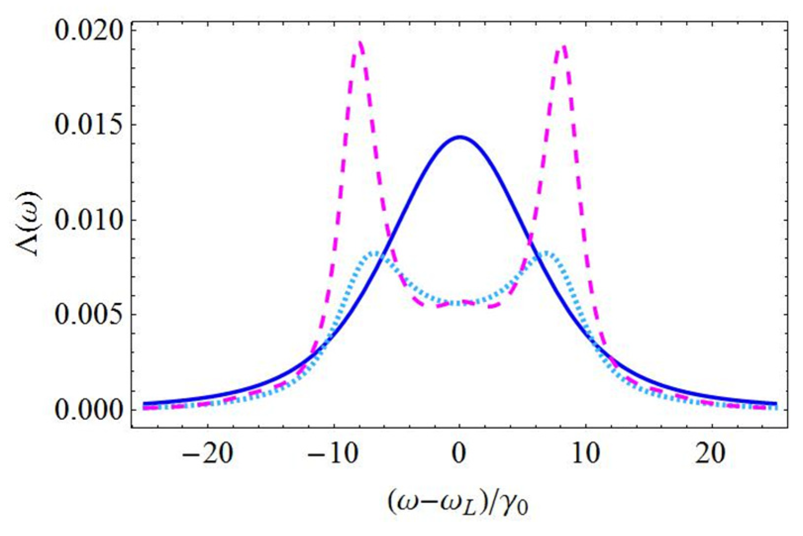
In Figure 4, we explore the dependence of the resonance fluorescence spectrum on the distance between the QE and the nanoparticle, for $\Omega =5{\gamma }_0$, ${\omega }_{21}=15{\gamma }_0$, in the case of a non-resonant laser field. We also assume that $\Delta ={\omega }_{21}/2$. Except for the principal resonance, which is centered around $\omega -{\omega }_L=0$, we can also derive analytical expressions for the positions of the sidebands: $\omega -{\omega }_L=\pm \sqrt{{\omega }_{21}^2+2{\Omega }^2}\simeq \pm 8.29{\gamma }_0$ and $\pm \sqrt{{\omega }_{21}^2+2{\Omega }^2}/2\simeq \pm 16.58{\gamma }_0$, based on the dressed state analysis. These values are consistent with our observations, for $d=50\mathrm{nm}$ (magenta dashed curve), due to the highly suppressed value of the decay rate, which is observed at high distances. For this specific value of the distance between the QE and the surface of the nanosphere, only the peaks of the inner doublet have a non-negligible amplitude, which, according to the analytical expression presented in the previous section, is equal to $0.0195$. The corresponding FWHM is approximately equal to $3.9{\gamma }_0$. For $d=27\mathrm{nm}$ (turquoise dotted curve), based on the analytical expressions, the amplitude of the resonances of the doublet and the corresponding FWHM becomes approximately equal to $0.0075{\gamma }_0$ and $7.1{\gamma }_0$, respectively. This significant broadening owes its presence to the amplification of the ${\Gamma }_{\perp }$ parameter. However, for even lower distances, as for instance in the case with $d=10\mathrm{nm}$ (blue solid curve), the analytical expressions are not accurate, since the condition $\sqrt{{\omega }_{21}^2+2{\Omega }^2}\gg \gamma$ is not valid, due to the substantial increase of the decay rate $\gamma$. In this limit case, the profile of the resonance fluorescence spectrum corresponds to a single significantly broadened Lorentzian-type peak, which is centered around $\omega ={\omega }_L$.

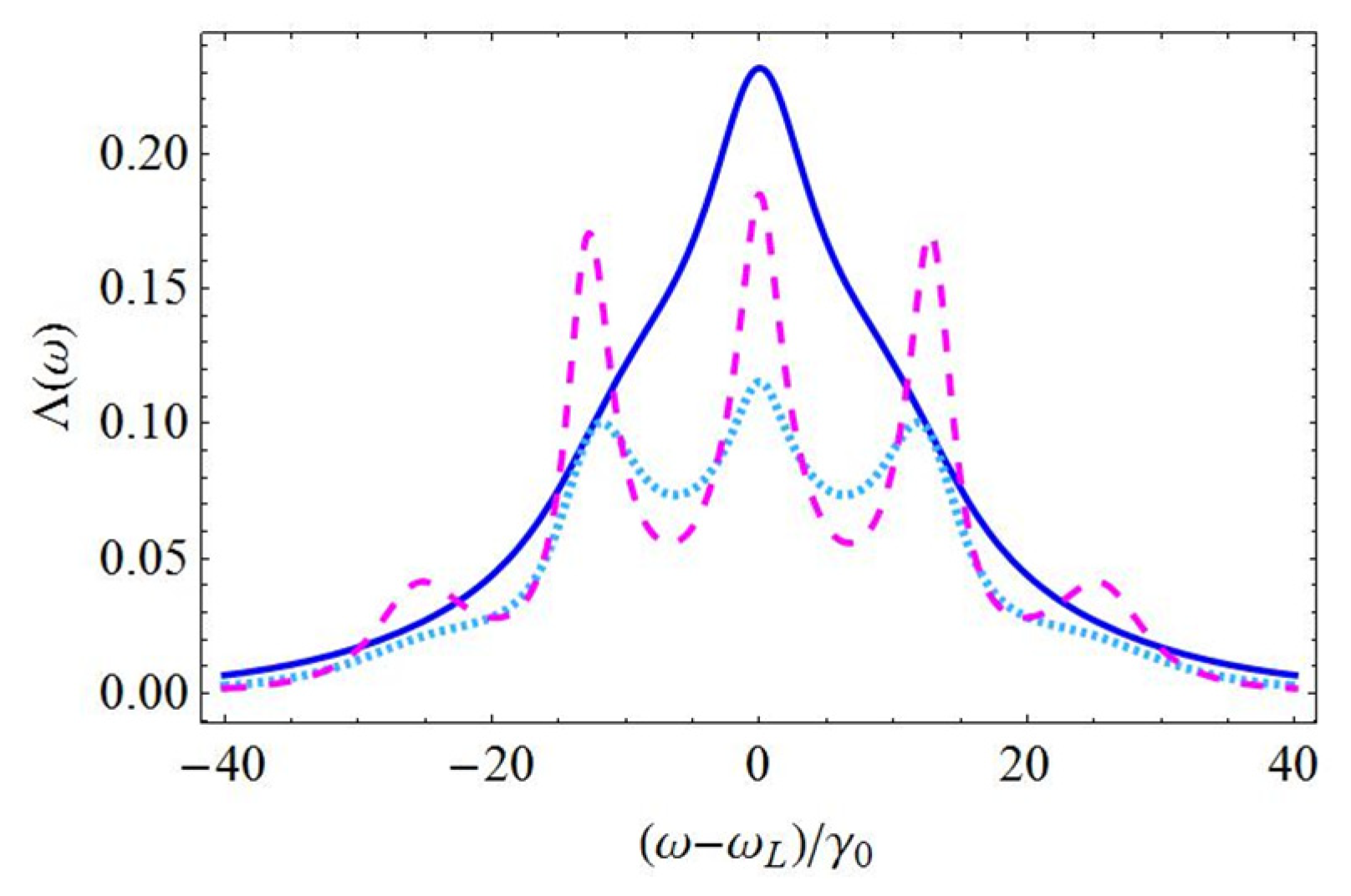
In Figure 5, we investigate the resonance fluorescence spectra, for $\Omega ={\omega }_{21}=15{\gamma }_0$ and $\Delta ={\omega }_{21}/2$. The resonance fluorescence spectrum is symmetric and is composed of a central peak $(\omega -{\omega }_L=0)$ and two doublets of sidebands ($\omega -{\omega }_L=\pm \sqrt{{\omega }_{21}^2+2{\Omega }^2}/2\simeq \pm 8.29{\gamma }_0$ and $\omega -{\omega }_L=\pm \sqrt{{\omega }_{21}^2+2{\Omega }^2}\simeq \pm 16.58{\gamma }_0$). For a distance $d$ between the QE and the surface of the nanoparticle equal to $50\mathrm{nm}$ (magenta dashed curve), the outer sidebands have an amplitude equal to $0.039$ and a FWHM equal to $8.5{\gamma }_0$. The central peak with amplitude equal to $0.166$ constitutes a superposition of two Lorentzian-type resonances, one with amplitude $0.095$ and FWHM = $6.6{\gamma }_0$ and one with amplitude $0.071$ and FWHM = $3.1{\gamma }_0$. The profile of each one of the inner sidebands is calculated by superimposing two Lorentzian functions with amplitudes $0.051$, $0.108$ and corresponding FWHM values equal to $4.5{\gamma }_0$ and $4{\gamma }_0$. For $d=27\mathrm{nm}$ (turquoise dotted curve), the amplitude of the resonances is substantially decreased and their FWHM is enhanced, as compared to the respective values identified for $d=50\mathrm{nm}$. This is due to the increase of both ${\Gamma }_{\perp }$ and ${\Gamma }_{\parallel }$. However, if we use the analytical expressions derived in the previous section, the results taken for the amplitude and the FWHM of the resonances are not accurate, since, due to the anisotropic Purcell effect, that is responsible for the increase of the decay rate at close distances, we are far from the accomplishment of the condition $\sqrt{{\omega }_{21}^2+2{\Omega }^2}\gg \gamma$. Moreover, the dressed state approximation is also crudely accurate, due to the same reason. Thus, the position of the resonances is somewhat transposed towards the center of the spectrum, as compared to the results reported in the case with $d=50\mathrm{nm}$ (magenta dashed curve). Finally, for $d=10\mathrm{nm}$ (blue solid curve), the extremely broadened central resonance, with amplitude equal to $0.231$, prevails over all the other resonances.

In Figure 6, we explore the characteristics of the resonance fluorescence spectrum, in the case of degenerate upper levels $({\omega }_{21}=0)$, for an exactly resonant laser field $(\Delta =0)$ with Rabi frequency $\Omega =15{\gamma }_0$. For this specific set of parameters, the dressed state analysis enables us to calculate the position of the resonances that correspond to $\omega -{\omega }_L=0$ and to $\omega -{\omega }_L=\pm \sqrt{2}\Omega$. Thus, a doublet of sideband peaks arises on the resonance fluorescence spectrum around the central resonance, creating a triple-peaked Mollow-type structure. Under the condition $\Omega \gg \sqrt{2}\gamma /2$, and since, in this case, we find ${\rho }_{aa}={\rho }_{cc}=0.5$ and ${\rho }_{bb}=0$, the exact shape of the spectrum is described by the following function:

$$\begin{array}{l}\Lambda (\omega )=\frac{{\Gamma }_{\perp }^2/2}{{\Gamma }_{\perp }^2+{(\omega -{\omega }_L)}^2}+\frac{{\left[3{\Gamma }_{\perp }/2\right]}^2/6}{{\left[3{\Gamma }_{\perp }/2\right]}^2+{\left[\left(\omega -{\omega }_L\right)-\sqrt{2}\Omega \right]}^2}+\\ {{}_{}}_{}{{}_{}}_{}{{}_{}}_{}{{}_{}}_{}{{}_{}}_{} +\frac{{\left[3{\Gamma }_{\perp }/2\right]}^2/6}{{\left[3{\Gamma }_{\perp }/2\right]}^2+{\left[\left(\omega -{\omega }_L\right)+\sqrt{2}\Omega \right]}^2}.\end{array}$$

(20)

According to the analytical expression of Equation (20), we deduce that all the resonances appearing on the spectrum are Lorentzian-shaped. The amplitude of the central peak is equal to $1/2$, while the amplitude of each one of the peaks of the doublet is equal to $1/6$. The FWHM of the central peak is $2{\Gamma }_{\perp }^{}$, while the FWHM of the sideband resonances is $3{\Gamma }_{\perp }^{}$. These values agree with our observations, for $d=50\mathrm{nm}$ (magenta dashed curve). However, for $d=27\mathrm{nm}$ (turquoise dotted curve), both the decay rate $\gamma$ and the coupling coefficient $\kappa$ are importantly increased. Since we cannot assume that $\Omega \gg \sqrt{2}\gamma /2$, the analytical expression given in Equation (20) is not valid. Also, the FWHM of the resonances exhibits a significant increase leading to the creation of a substantial overlap between the individual resonances. Finally, at very low distances, as in the case corresponding to $d=10\mathrm{nm}$, which is depicted with the blue solid curve, the sideband resonances are annihilated, the amplitude of the central peak is strongly suppressed, while its FWHM is importantly augmented, as a result of the substantial amplification of the $\gamma$ and $\kappa$ parameters.

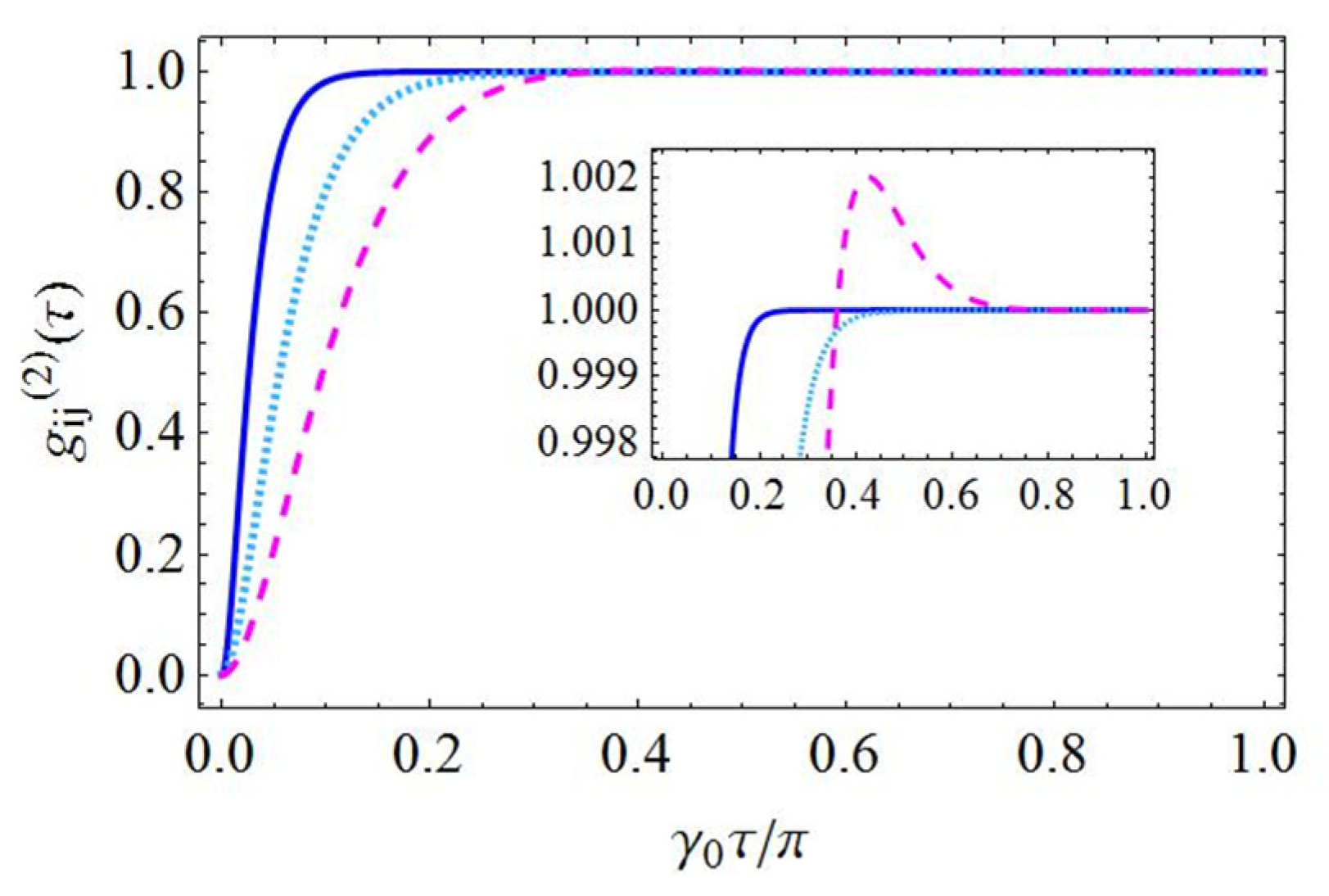
In Figure 7, we investigate the second-order (intensity-intensity) correlation functions, for a strong and exactly resonant $(\Delta =0)$ laser field, with Rabi frequency $\Omega$ equal to $40{\gamma }_0$. Here, we investigate the degenerate case $({\omega }_{21}=0)$ and, thus, the functional forms of $g_{ij}^{(2)}(\tau )$ are expected to be identical to the ones taken for a two-level system. We observe that, as long as the Rabi oscillation of the transition dipole moments prevail over the spontaneous decay process, the second-order correlation functions evolve over time in an oscillatory manner. More explicitly, they exhibit a symmetric oscillatory pattern with mean value equal to unity and period equal to $\sqrt{2}\pi /\Omega$, independent of the distance that separates the QE from the gold nanosphere (blue solid curve, turquoise dotted curve and magenta dashed curve respectively correspond to $d=10,27$ and $50\mathrm{nm}$). As the QE is brought closer to the gold nanosphere, the spontaneous emission rate ${\Gamma }_{\perp }$ is substantially increased ($\simeq 3.11{\gamma }_0$, for $d=50\mathrm{nm}$, $\simeq 6.60{\gamma }_0$ for $d=27\mathrm{nm}$ and $\simeq 14.83{\gamma }_0$, for $d=10\mathrm{nm}$) and, due to this effect, the damping coefficient increases monotonically. In Figure 7, it becomes evident that the time which is required in order to pass from the antibunching to the bunching region (crossing time) does not depend on the interparticle distance. The zero value at $\tau =0$ expresses the zero probability of identifying two fluorescent photons simultaneously, due to the depletion of the system. If we decrease the intensity of the incident field at a high extent (practically when takes values below $\Omega <5{\gamma }_0$, when $d=50\mathrm{nm}$), the damping rate presents an important suppression. In this specific case, which will be investigated in Figure 9, the second-order correlation functions always remain in the antibunching region and, thus, the successive emission of another fluorescent photon is hindered.

The second-order correlation functions are explored in the non-degenerate quantum system with frequency mismatch ${\omega }_{21}$ equal to $15{\gamma }_0$, in Figure 8, where we also assume that the detuning of the incident laser field satisfies the condition $\Delta ={\omega }_{21}/2$. The rest physical parameters take the same values as in Figure 7. In the case of high distances, as for $d=50\mathrm{nm}$ (magenta dashed curve), it becomes apparent that that the time evolution of $g_{ij}^{(2)}(\tau )$ is a result of a superposition of two discrete oscillations with angular frequencies ${\omega }_1=\sqrt{2}\Omega$ and ${\omega }_2={\omega }_1/2$. This effect was thoroughly explained in Ref. [40]. As in the case of two degenerate upper levels which were excited by a laser field found at exact resonance with the corresponding transitions (Figure 7), the highest fluctuations of the second-order correlation function are exhibited at high distances, where ${\Gamma }_{\perp }$ is importantly reduced. However, their amplitude is slightly reduced, since the combined oscillations of the coherences correspond to opposite phases. Here, both in the long distance regime ($d=50\mathrm{nm}$: magenta dashed curve), as well as for intermediate values of the interparticle distance, as for $d=27\mathrm{nm}$ (turquoise dotted curve), the crossing time from antibunching to bunching takes the same value that is approximately equal to the one identified in Figure 7. In the first case, we take $g_{ij}^{(2)}(\tau )>1$, within well-specified time intervals, as long as $\tau <0.26\pi /{\gamma }_0$, while, in the second case, the bunching is not significant and it can only be obtained when $\tau$ lies below $0.052\pi /{\gamma }_0$. Since the blue solid curve ($d={10}_{} \mathrm{nm}$) lies below unity, we deduce that, at low distances, the consecutive emission of two fluorescence photons with a delay less than the spontaneous decay time is unlikely.

In Figure 9 and Figure 10, we consider a weak laser field with corresponding Rabi frequency $\Omega =2{\gamma }_0$. In Figure 9, the incident field is exactly tuned $(\Delta =0)$ from the ground state $\left|0\right.〉$ to the degenerate upper energy levels $\left|1\right.〉$ and $\left|2\right.〉$. Here, the second-order correlation functions increase monotonically with time, remaining in the antibunching region all the time, and finally reaches unity at a higher rate for $d=10\mathrm{nm}$ (blue solid curve), rather than for $d=27\mathrm{nm}$ (turquoise dotted curve). In the case with $d=50\mathrm{nm}$ (magenta dashed curve) that corresponds to importantly suppressed values of the decay rate, the coupling coefficients, $g_{ij}^{(2)}(\tau )$ presents a highly-damped oscillatory behavior, with crossing time to the bunching region $\tau =0.36\pi /{\gamma }_0$. However, if we further decrease the intensity of the laser field so that $\Omega ={\gamma }_0$, the functional form of $g_{ij}^{(2)}(\tau )$, for $d=50\mathrm{nm}$, is found to be similar to the one exhibited for lower distances, since it never crosses the antibunching-bunching border (not shown here).

In Figure 10, we take ${\omega }_{21}=15{\gamma }_0$ and $\Delta ={\omega }_{21}/2$. For this set of parameters, still remaining in the weak field regime, the distance separating the QE and the plasmonic nanostructure seems to play a crucial role to the time evolution of the second-order correlation function. More specifically, while for $d=10\mathrm{nm}$ (blue solid curve) the time evolution of the photon statistics is similar to the one exhibited in the case of a degenerate system found at exact resonance (Figure 9), for higher distances, we note that $g_{ij}^{(2)}$ evolves in an oscillatory manner. For $d=10\mathrm{nm}$, the spontaneous decay process is responsible for the damping of $g_{ij}^{(2)}$, since it takes place at a rate that is approximately equal to $7.87{\gamma }_0$, which is high as compared to the value of the Rabi frequency of the driving field. However, for $d=27\mathrm{nm}$ (turquoise dotted curve) and $d=50\mathrm{nm}$ (magenta dashed curve), the Rabi oscillations are not washed out, since the corresponding decay rates ($3.50{\gamma }_0$ and $1.82{\gamma }_0$) are comparable to value of the Rabi frequency. We observe that the period of the oscillations detected on the second-order correlation function is importantly increased as compared to the strong field regime explored in Figure 7, due to the substantial decrease of the Rabi frequency, while the crossing time increases monotonically with the interparticle distance ($\tau =0.080\pi /{\gamma }_0$, for $d=27\mathrm{nm}$ and $\tau =0.056\pi /{\gamma }_0$, for $d=50\mathrm{nm}$).

Before closing, we would like to mention that the above results shows that the present system behaves quite different from relevant earlier works. For example, in comparison with the system of the two-level QE coupled to a metal nanosphere [1,2,3,4,6,7,8,10,11,13,14,16], both the resonance fluorescence spectrum and the two-time intensity correlation functions of the fluorescent field show different behavior, as in this case they depend strongly on the additional features of the studied system, namely the coupling of the driving electromagnetic field simultaneously to the two different transitions $\left|0\right.〉\to \left|1\right.〉$ and $\left|0\right.〉\to \left|2\right.〉$, the coupling term $\kappa$ which gives the effects of quantum interference in spontaneous emission, and its value also depends on the presence of the metal nanosphere, as well as the energy difference between the two upper levels.

Furthermore, in comparison now with the behavior of the intensity-intensity correlation function of the fluorescent photons in the V-type QE near a periodic metal-dielectric nanostructure, which was presented in Ref. [22], the currently studied system is a simpler system, hence it is easier experimentally realizable; it is also a basic system, as the spherical metal nanoparticle is the most studied plasmonic nanostructure in this area of studies [1,2,3,4,6,7,8,10,11,13,14,16,17,20,21,23]. In addition, the behavior of the decay rates is significantly different, as compared to the case of the periodic metal-dielectric nanostructure, the degree of quantum interference is significantly larger (larger than 0.95), while, at the same time, the values of both ${\Gamma }_{\perp }$ and ${\Gamma }_{\parallel }$ can be lower than ${\gamma }_0$ [22,24,25,34], within a specific region of distances between the QE and the plasmonic nanostructure, where we obtain $\gamma <{\gamma }_0$, that also alters the obtained results. Finally, in comparison to the studies of other three-level QEs near a plasmonic nanostructure, like the cascade three-level structure [19,20] and the Λ-type three-level structure [21], the previously studied systems neither induce effects of quantum interference in spontaneous emission nor study a case where there is a simultaneous driving of both transitions by a single electromagnetic field, as we do in the present work.

4. Conclusions

We have studied the resonant fluorescence spectrum and the two-time intensity correlation functions of the fluorescent field emitted by an externally driven V-type QE which is placed near a gold nanosphere. More explicitly, we examine the influence of the interparticle distance, as well as of a series of other physical parameters that describe the system, including the intensity of the applied laser field, its detuning from resonance and the spacing between the upper levels on the shape of the spectral profiles, as well as on the fluorescent photon statistics. Based on a dressed state analysis, we demonstrate that the resonant fluorescence spectrum is composed of a set of Lorentzian-shaped resonances with well-specified positions and widths. The V-type system also shows quantum interference in spontaneous emission due to the anisotropic Purcell effect.

For a QE with degenerate excited levels which is placed in the vicinity of the metal nanosphere and is driven at exact resonance by the laser field, we find a characteristic triple-peaked Mollow-type resonance fluorescence spectral profile, where the central peak is dominant. In the strong driving field regime, the resonant fluorescence spectrum is five-peaked, while, in the weak field regime, we take a triple-peaked spectrum which practically appears to be double-peaked in the limit case where the spacing between the upper levels is high as compared to the Rabi frequency. For high distances between the QE and the metal nanosphere, the spectrum becomes single peaked, for every set of the physical parameters. In the strong driving field regime, we conclude that the distance between the QE and the metal nanoparticle modifies the damping rate of the Rabi oscillations detected on the two-time correlation functions, while the crossing time from antibunching to bunching is unaffected. However, for a non-degenerate system interacting with an off-resonant pump field, the system can remain in the antibunching region all the time, in the case of small distances. In the weak driving field regime, the period of the Rabi oscillations is increased and in the specific case of a degenerate system found at exact resonance with the applied laser field, the system does not present transition from the bunching to the antibunching region, for any distance between the QE and the gold nanosphere.