Article

Flexible Plenoptic X-ray Microscopy

1
Elettra-Sincrotrone Trieste S.C.p.A., 34149 Trieste, Italy
2
Institute of Materials Physics, Helmholtz-Zentrum Hereon, 21502 Geesthacht, Germany
3
Laboratoire d’Optique Appliquée UMR7639, ENSTA, CNRS-Ecole Polytechnique IP Paris, 91762 Palaiseau, France
4
Centrum Wiskunde & Informatica (CWI), 1098 XG Amsterdam, The Netherlands
5
Imagine Optic, 33400 Talence, France
6
Deutsches Elektronen-Synchrotron, DESY, 22607 Hamburg, Germany
7
Instituto de Plasmas e Fusão Nuclear, IST Lisboa, 1049-001 Lisbon, Portugal
8
European Synchrotron Radiation Facility, 38043 Grenoble, France
*
Author to whom correspondence should be addressed.
Photonics 2022, 9(2), 98; https://doi.org/10.3390/photonics9020098
Submission received: 17 January 2022 / Revised: 1 February 2022 / Accepted: 2 February 2022 / Published: 8 February 2022
(This article belongs to the Special Issue Advances in X-ray Optics)

Abstract

:
X-ray computed tomography (CT) is an invaluable technique for generating three-dimensional (3D) images of inert or living specimens. X-ray CT is used in many scientific, industrial, and societal fields. Compared to conventional 2D X-ray imaging, CT requires longer acquisition times because up to several thousand projections are required for reconstructing a single high-resolution 3D volume. Plenoptic imaging—an emerging technology in visible light field photography—highlights the potential of capturing quasi-3D information with a single exposure. Here, we show the first demonstration of a flexible plenoptic microscope operating with hard X-rays; it is used to computationally reconstruct images at different depths along the optical axis. The experimental results are consistent with the expected axial refocusing, precision, and spatial resolution. Thus, this proof-of-concept experiment opens the horizons to quasi-3D X-ray imaging, without sample rotation, with spatial resolution of a few hundred nanometres.

1. Introduction

X-ray computed tomography (CT) is a powerful three-dimensional (3D) imaging method for the non-invasive inner exploration of materials [1] and biological samples [2]. X-ray CT at storage ring sources is traditionally considered a benchmark for investigations in the soft [3] and hard [4] X-ray regimes; it enables access to length scales as low as 1 µm and 50 nm spatial resolutions in the fields of microtomography [5] and nanotomography [6], respectively. However, X-ray CT inevitably requires up to thousands of projections to build a single high-resolution 3D volumetric image.
The strong reduction in the number of projections for achieving 3D or quasi-3D images is an important objective today. Quasi-3D encompasses all of the techniques—such as stereoscopy or holography—that partially sample the object in 3D. The advantage of single-shot quasi-3D imaging over traditional CT is twofold: (a) it is suitable for fast dynamic processes, and (b) it intrinsically avoids the need to rotate the sample. (a) The temporal resolution of an acquisition is reduced from the duration of a scan to the duration of a single exposure. This can signify the ability to track flow dynamics in perfusion CT, intravascular tools in interventional imaging, changes induced by fast chemical reactions in operating energy storage devices, or crack nucleation and propagation in material deformation experiments, all in 3D. (b) The required sample rotation in synchrotron CT can interact with fluid samples, and can strongly influence their state and behaviour. The ability to resolve their 3D structure without rotating them can unlock unprecedented studies of their unaltered functioning state (e.g., particle image velocimetry of opaque fluids); moreover, it can enable the reconstruction of specimens with anisotropic or non-cylindrical shape (e.g., biological sample slices).
Several attempts have been made to recover quasi-3D information from a pair of views using X-ray stereoscopy [7,8] and a single sample orientation using X-ray ankylography [9]. Recently, visible plenoptic imaging has attracted attention given its ability to record depth information in one view. From a single exposure, plenoptic imaging enables the generation of a stack of images located at several distances along the optical axis. The technique is based on a combination of an objective lens and an array of microlenses [10,11]. To date, this method is still restricted to visible light, due to the complexity of using X-ray optics. In the literature there can be found numerical simulations emulating the operating mode of an X-ray plenoptic system with limited-angle tomography setups [12,13]. A preliminary experimental demonstration of plenoptic X-ray imaging was performed by Sowa et al. in so-called multipoint projection geometry [14,15]. Using a laboratory source, Sowa et al. developed an X-ray plenoptic microscope version based on polycapillary focusing optics, instead of using a microlens array [14]. As consequence, the setup shows a limited depth resolution due to the limited angular sampling of the polycapillary devices and a lateral resolution restricted to micro-sized sources [14]. This article shows an advancement of the optical design required for the implementation of an X-ray plenoptic microscope, thus enabling an increase in the angular and spatial sampling of the incoming X-rays, as well as enhancement of the refocusing ability. Here, the first X-ray plenoptic microscope based on an X-ray optics array is presented and used in a flexible configuration [16]. The microscope was created by combining a Fresnel zone plate (FZP)—i.e., the objective lens—with a movable array of FZPs—i.e., the microlens array—placed in front of a detector. This implementation is flexible, enabling different plenoptic imaging configurations on the same setup. By slightly modifying the distances between the optical elements, it is possible to switch from the focused plenoptic imaging geometry [11] to the classical plenoptic imaging configuration [10], both known in visible light photography. Any change of distances implies a change of angular and spatial light field sampling, and of the related lateral and longitudinal resolutions. Therefore, the different microscope parameters can be adjusted according to the acquisition needs. The X-ray microscope geometry adopted in this work reproduces the focused plenoptic camera configuration [11]. The X-ray plenoptic microscope implemented here was thoroughly tested by imaging USAF test targets placed at different positions, and by computationally refocusing the recorded raw plenoptic images. To increase the spatial sampling, the image acquisition was performed by scanning the FZP array 16 times. Finally, the acquired micro-images were stitched leading to better resolved image features compared to the initial number of available micro-images. The achieved spatial and longitudinal resolutions were measured on the refocused images considering different approaches, and the estimated values were compared to the theoretical calculations.

2. Materials and Methods

2.1. Experimental Setup

The X-ray plenoptic imaging demonstration was carried out at 11 keV by modifying the transmission X-ray microscope (TXM) available in the nanotomography experimental hutch [17] of the P05 imaging beamline [18], at the PETRA III storage ring at the Deutsches Elektronen-Synchrotron (DESY) in Hamburg, Germany. The P05 beamline is operated by the Helmholtz-Zentrum Hereon. The nanotomography setup encompasses a granite optical bench (6.8 m long) equipped with 4 air-bearing movable sliders for the positioning of the microscope components. Figure 1 shows the adopted experimental configuration (an additional picture of the setup is illustrated in Appendix A, Figure A1). The setup was arranged by combining different diffractive elements: a beam shaper condensing optics for illuminating the sample [19,20], a single FZP as the objective lens, and 9 × 9 FZPs as the microlens array. The used beam shaper was 1.8 mm in diameter, with 50 μm2 subfields and 50 nm outermost zone width. The single FZP (280 µm in diameter, outer zone width equal to 50 nm, and 0.001 numerical aperture) was used as the objective lens of the transmission X-ray microscope (TXM). Both the beam shaper and objective lens FZP were designed and fabricated at the Paul Scherrer Institut (PSI) in Villigen, Switzerland. An array of 9 × 9 FZPs—each with a diameter of 100 µm, an outermost zone of 100 nm, a numerical aperture of 0.0005, and 250 gold zones—was placed in front of the detector. The FZP array was fabricated on a 100 nm thick silicon nitride membrane support window with a 5 mm × 5 mm substrate frame. The microlenses were placed on a Cartesian grid, with a zone plate spacing of 10 µm and periodicity (i.e., centre-to-centre distance of two adjacent FZPs) of 110 µm. The array was manufactured with a gold thickness equal to 1500 nm. The FZP array was installed downstream of the main lens, prior to the detector. Specific details related to the used optics are available in the Materials and Methods section and in Appendix A, Figure A2. In order to block the zero order, a 400 µm diameter gold beam stop (provided by the beamline) was installed downstream of the beam shaper, while a specifically designed array of gold beam blockers was placed downstream of the FZP array on a separate holder. These gold blockers were manufactured with an inner diameter equal to 35 µm, an outer diameter equal to 92 µm, and a gold thickness equal to 10 µm. Both the FZP array and the array of gold beam blockers were specially designed for this experiment and produced by Applied Nanotools Inc. (city, state, country) (ANT, Edmonton, Alberta T6G 2M9, Canada). The beam shaper/beam stop combination produced a hollow cone illumination, illuminating an area of 50 µm × 50 µm at the sample plane. In addition, order sorting apertures (OSAs) were used around the single FZP for blocking higher diffractive orders. The sample consisted of two conventional USAF 1951 targets with parallel and perpendicular lines of different width and spacing (elbow pattern; see Figure A3 in Appendix A), mounted in a “T” shape and slightly overlapping. The two test targets were Au structures (600 nm thick) on a silicon nitrate membrane, and were purchased from ANT. The two targets were placed along the optical axis at 128.7 ± 0.2 mm and 130.0 ± 0.2 mm from the main lens, respectively. The distances from the objective lens to the lens array and the lens array to the detector were 3846 ± 10 mm and 111.8 ± 0.5 mm, respectively. The separation distance between the targets (1.3 mm) was larger than the theoretical field depth of 300 µm [21]. The distances were chosen in order to create the image of the sample at an intermediate plane between the main lens and the microlens array, and then onto the detector, as shown in Figure 1.
This geometry corresponds to the so-called focused plenoptic camera configuration [11]. It was chosen over the unfocused camera [10] due to its flexibility and higher spatial resolution around the focal plane of the main lens. The images were acquired with a PCO.edge 4.2 CMOS camera (2048 × 2048 pixels) integrated with a 50 µm thick LuAG(Ce) scintillating crystal and coupled with a visible microscope with 7× optical magnification; this setting led to an effective pixel size of 0.92 × 0.92 µm2. The beam shaper and beam stop were accommodated on the first slider of the granite bench, the targets on the high-precision rotation stage on the second slider, the objective FZP on the third, and the FZP array and the detector were installed on the fourth (Figure A1, Appendix A). The experiment was performed at an energy of 11 keV and with a flux at the rate of 1012 photons/second. At this energy, the focal length of the main FZP was 124 mm and the focal length of the FZP array was 88.73 mm. Each single image was acquired with 5 s exposure time. The dataset acquired with 9 × 9 FZPs comprised 40 images and 16 flat fields, and was obtained after a total exposure time equal to 280 s. The stitching datasets consisted of 16 positions, each containing 10 raw images and 4 flat fields. The total exposure time for stitching was 1120 s.

2.2. Data Processing

For each configuration, 10 images were acquired and then averaged to create an image with a better signal-to-noise-ratio. Reference (flat-field) images were acquired without the sample. The average of four reference images was then used for a normalisation step, to correct for beam inconsistencies and motor errors. This normalisation enables the extraction of the useful signal from the background. This pre-processing step was executed for each position of the microlens array separately. Finally, the exact centre of each micro-image was found manually, allowing us to extract all of the micro-images from the different raw images. The micro-images were then combined together to form a dataset with 36 × 36 micro-images used as inputs to the refocusing algorithm.

2.3. Dedicated Software to Generate Synthetic or Refocused Experimental Raw Plenoptic Images

The refocusing algorithm is at the heart of plenoptic imaging, since it enables the raw array of micro-images to be transformed into full images refocused at any distance from the camera. A new refocusing algorithm [21] has been developed that overcomes the distinction between traditional [10] and focused algorithms [11] by unifying both approaches. The algorithm is based on a unique set of equations describing the propagation of the light rays in a plenoptic setup composed of an objective lens, a microlens array, and a detector. The set of equations defines the transformation between object-space and sensor-space rays, based on geometric optics applied on both the objective lens and the microlens array. In this approach, the ray propagation is given as a function of the physical distances of the setup, without assuming a specific configuration or any relationship between the distances and the parameters. It is thus physically based, and can be used for data acquired in either the traditional or focused configurations.
Based on this set of equations, two algorithms were implemented. The refocusing process starts with the backpropagation of the acquired data from sensor space to object space, at a depth chosen by the user; it is then followed by the combination of all of the angular information converging at the same spatial position, mimicking the light integration of a sensor pixel. A simulation algorithm was also implemented, allowing us to generate synthetic data from an object placed in object space. The simulation process is reversed compared to the refocusing algorithm—the data are projected from object space to sensor space using the defined set of equations, before their integration at the sensor plane to generate the synthetic plenoptic image [22]. The parameterisation together with the integration constitutes a unique method that is valid regardless of the configuration in which the data were acquired.

3. Results

Figure 2a shows characteristic features in the raw plenoptic images produced by the X-ray microlens array. Due to a mismatch in size between the OSA around the main FZP and the microlenses’ diameter, several grey lines corresponding to 0th order transmission can be observed. Superimposed on these lines are circles with black structures at their centres. A closer look at these circles (Figure 2b) reveals that the inner black structures are images of a small part of the sample produced by the +1st diffraction order (called micro-images). The use of a beam stop array placed after the microlens array prevents the 0th order (red dotted circle in Figure 2b) from mixing with the +1st order (yellow dotted circle in Figure 2b). The plenoptic information is contained only in the yellow circle (1st order). Only the signal from these pixels can be used for data treatment. The objective lens magnifies the front and the back targets by approximately 30.6 and 29.6 times, respectively. The microlenses magnify by a factor 0.2, leading to a total magnification of ~6. The beam divergence at the objective lens exit was estimated at around 0.3 mrad, while for the microlenses, the entrance divergence was 0.11 mrad. This mismatch of divergences generated small micro-images, ~20 µm in diameter (i.e., 22 pixels), separated by a distance corresponding to the microlens pitch of 110 µm (Figure 2a). In order to achieve a denser sampling, a new image was taken with a shift of the microlens array by a quarter of the inter-lens spacing, i.e., by 27.5 µm; these two images were then merged. This procedure was repeated three times in both the horizontal and vertical directions, generating a stitched plenoptic raw image, composed of 36 × 36 micro-images (Figure 2c).
The raw data were treated using a dedicated algorithm (see Materials and Methods) that can operate on all plenoptic configurations (focused and unfocused) [22].
Figure 3 shows the comparison between the images obtained using the objective lens only (Figure 3a), using the objective lens and the microlens array corresponding to classical plenoptic imaging (Figure 3b), and the resulting plenoptic image after stitching (Figure 3c).
The three images were obtained with the same position of the targets adjusted such that the first image is in focus, thus placed at a position of approximately Z0exp = 128.7 mm from the objective lens. However, for Figure 3a the detector was situated at the position of the intermediate image plane (Figure 1), while it was moved further from the objective lens in order to insert the microlens array for the plenoptic configuration. This leads to different magnifications in Figure 3a–c. The 2 µm spaced lines of the first and second targets are recognizable on the right part of the reconstructed plenoptic image (Figure 3b); they appear dashed, and not plain as they are in reality (Figure 3a). In addition, on the left-hand side the number “2” of the first target (TP1) is barely visible, and the lines of the back target (TP2) with spacing lower than 1 µm are not resolved; this is due to the low number of microlenses (9 × 9) used for sampling the intermediate image created by the main lens. Figure 3c displays the reconstructed image of the targets using the synthetic 36 × 36 micro-images. Compared to Figure 3b, the improvement is striking. The noise has been strongly reduced thanks to the addition of 16 images. In addition, the true image can now be resolved, showing the plain lines instead of the dashed lines seen in Figure 3b. Additionally, the number “2” is now clear and readable (Figure 3c). The image of the back target remains blurred due to being out of focus. This first step of the study shows the quality of the plenoptic reconstruction.
The first dataset was taken with the first test target (TP1) situated close to the best experimental in-focus position. The second target (TP2) was placed 1.3 mm from TP1. An image stack was computationally produced by varying the focus position of TP1 from 128.6 mm to 129.5 mm in 100 µm steps in order to find its most accurate in-focus position. Four consecutive refocused images of TP1 are displayed in Figure 4a,d,g,j, within a 0.3 mm long range. Figure 4d,g exhibit images of TP1 with the highest contrast over the full scan, implying that both refocused planes can be considered to be in focus at the same time. This was expected, since the separation of these two reconstruction planes is lower than the theoretical depth of field [22], found to be 0.3 mm in this demonstration. Image processing allowed Z0exp to be defined as 128.75 ± 0.05 mm. In all of the computationally refocused positions, TP2 was blurred, since it was placed ~1 mm away from the depth of field of the whole plenoptic system. Experimental results were compared with simulated images. To precisely characterise the plenoptic X-ray microscope, the algorithm used for reconstructing the data was reversed, allowing us to generate synthetic plenoptic raw images [21,22] (see Materials and Methods) of the three TP1 bars labelled 1, 2, and 3 in Figure 4g. All parameters of the simulation were chosen to be the same as in the experiment, considering TP1 placed at Z0exp = 128.7 mm. The simulated refocused images are displayed in Figure 4c,f,i,l, and are a zoomed view of TP1’s bars. The simulated images of the bars are compared with the magnified views of the refocused images of the bars shown in Figure 4b,e,h,k. The visual agreement between modelling and experiment is good for all of the refocused positions. The ability of the plenoptic X-ray microscope to perform digital refocusing and defocusing from a single acquisition was subsequently tested. The assembly of TP1 and TP2 was positioned at different distances from the FZP. For each raw image acquired, a refocused image stack was reconstructed by the refocusing algorithm, and the image showing the highest contrast on either TP1 or TP2 was selected. The highest contrast was determined by visual inspection, as there was a marked difference between the in-focus image corresponding to the highest contrast and the other unfocused images.
Figure 5 shows three refocused images acquired at different positions of the assembly of TP1 and TP2. The first position labelled “0” in Figure 5 corresponds to Figure 4d at Z0exp = 128.7 mm. Moving the target assembly closer to the main lens by 0.5 mm (position 1, Figure 5), both targets appear out of focus, although the image of TP2 is slightly sharper and more resolved compared to the structures in Figure 4d,g. Moving the assembly once more towards the main lens by 0.5 mm (position 2, Figure 5), the image of TP1 becomes totally blurred. Due to a small change in contrast between positions 1 and 2, section profiles were not sufficient to define the best focusing distance for TP2 (see Appendix A, Figure A4). Thus, the long bar of TP2, indicated by the yellow arrow in each sub-image of Figure 5, was identified as a reference feature to determine the focusing trend for TP2. While this line is single (see Appendix A, Figure A3) and well defined at position 2, it looks doubled at position 1, and even more doubled at position 0. This is evidence that TP2 is defocused at positions 0 and 1, while its sharpness improves moving towards position 2; however, position 2 is not quite its exact focal plane. Similarly, the orange arrow indicates the focusing evolution of TP1 for the three different cases. The chart border, indicated by the orange arrow, is sharp and single at position 0, and then it becomes doubled at position 2. In this condition, TP2 was positioned at 0.3 mm from the initial position of TP1. This indicates a depth of field smaller than 0.3 mm, and confirms the plane of best focus to be around Z0 = 128.75 mm. TP1 and TP2 are never completely in focus at the same time.
Spatial resolution is a standard parameter used to find the focal plane for classical cameras, and it is used here to confirm the position of the best digitally refocused plane. The spatial resolution was estimated by two independent techniques giving similar values. The first estimation was done by estimating the point-spread function (PSF) directly from the gradient of the intensity along a line crossing a sharp edge. This measurement was performed on the large bars labelled 5 and 6 in Figure 4g. The derivative generated a Gaussian shape for the PSF with a resolution of ~420 ± 60 nm. The resolution estimation was obtained averaging over five pixels. However, the signal-to-noise ratio was too low (2–3) for ensuring an accurate measurement. Alternatively, it can be considered that the narrower black bars (labelled 1–4 in Figure 4g) are the convolution of a 1 µm width square function with a Gaussian PSF [23]. Thus, the second estimation was performed by convolving the 1 µm bars (labelled 1 and 4) with a Gaussian function of different widths. The results are full width at half-maximum values, and are displayed in Figure 6a,b. The measured resolution varies from 350 nm ± 50 nm to 660 nm ± 50 nm.
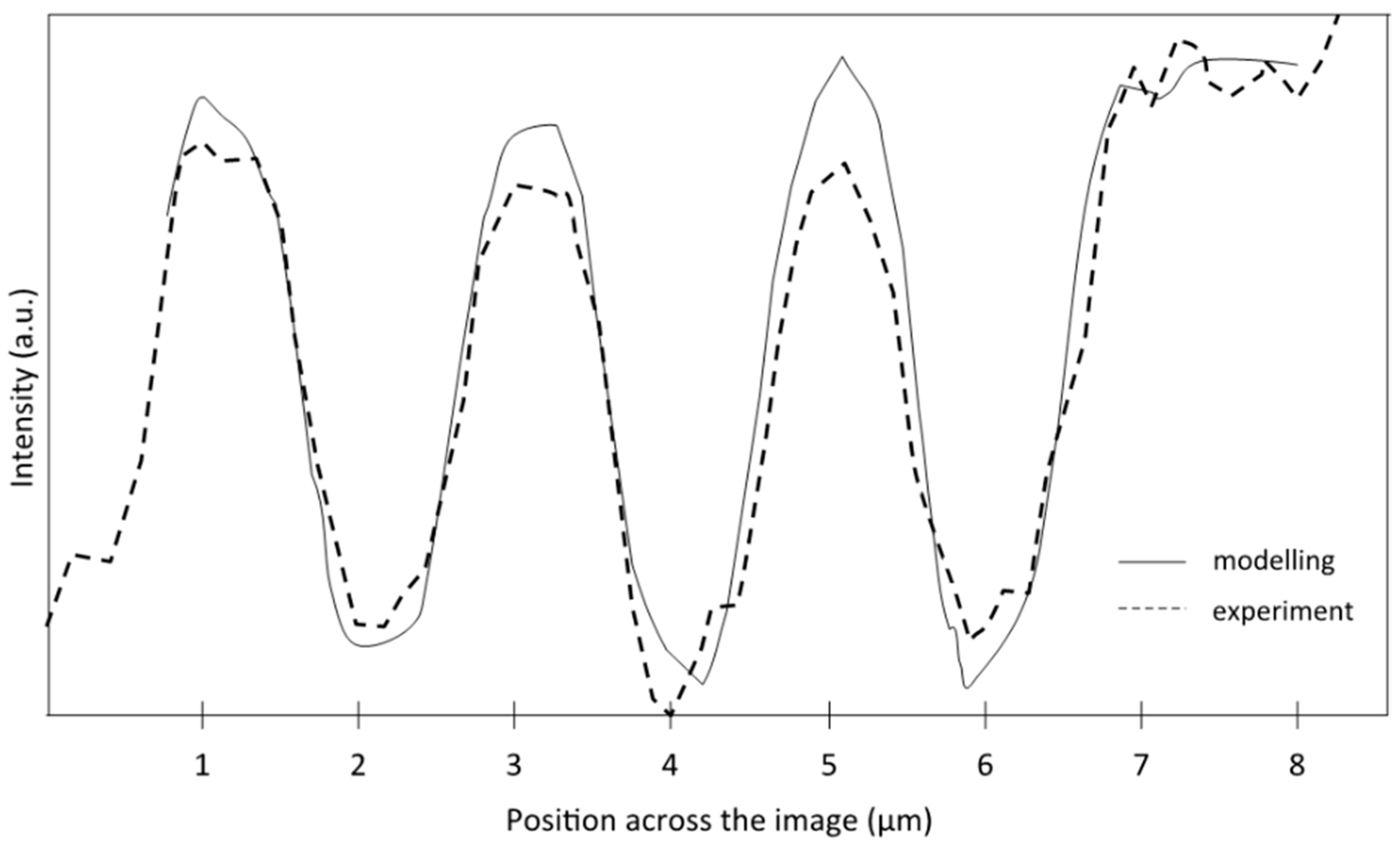
Figure 7 displays the cross-sections of bars 1–3, extracted from both experimental and numerical images (Figure 4h,i, respectively) obtained at Z0 = 128.8 mm, corresponding to the plane of best focus. The theoretically computed curve is in good agreement with the experimental measurement. It is worth noting that the shape of the three bars obtained experimentally is accurately reproduced numerically. As shown in Figure 6, the modification of the bar shape from a top hat (left and centre bars) to a Gaussian shape (right bar) indicates a variation in the spatial resolution across the image.
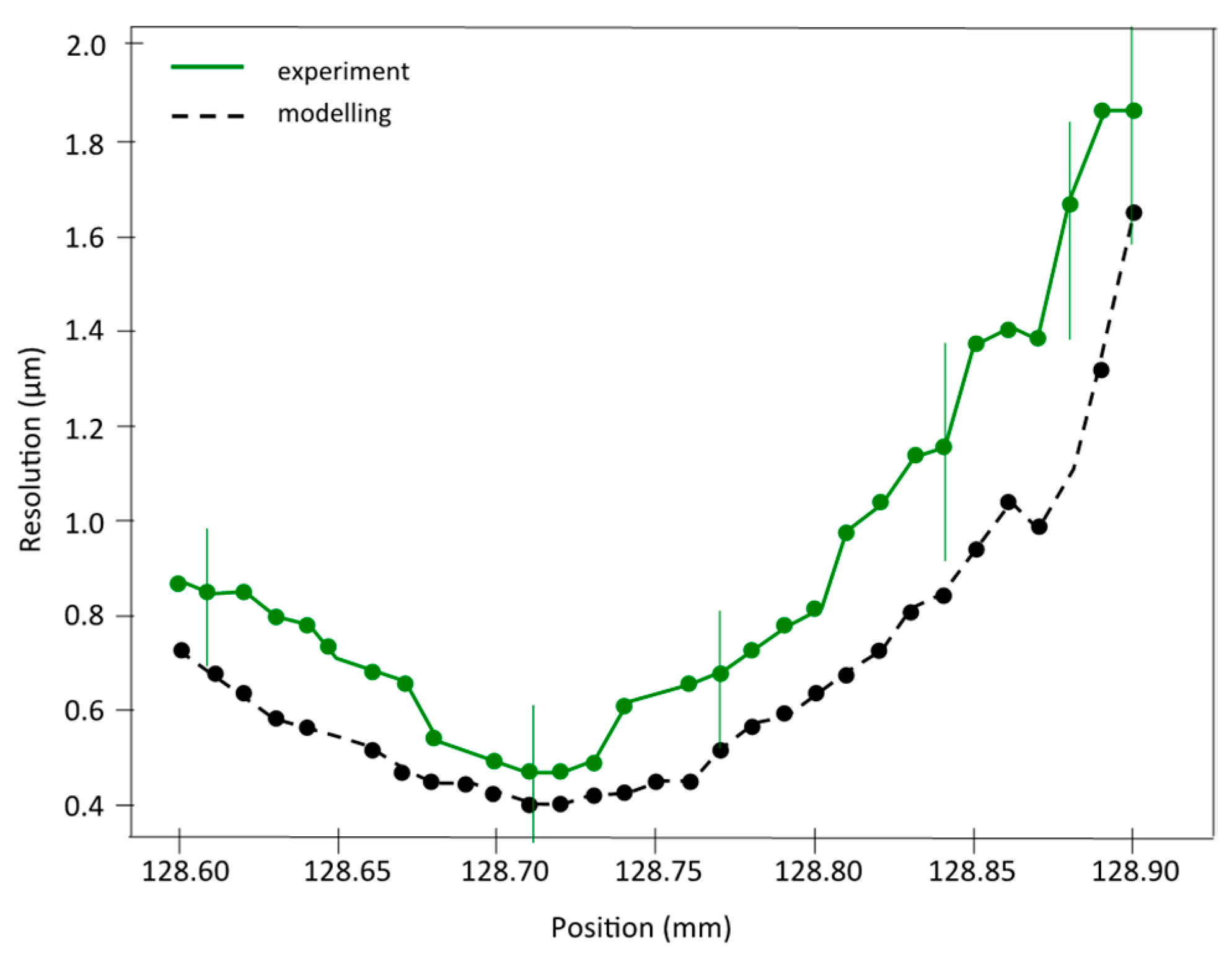
As a final step of the study of this plenoptic X-ray microscope, the longitudinal resolution of the refocused images was investigated by scanning the spatial resolution over a wide range of refocused positions. Figure 8 displays both numerical and experimental spatial resolutions versus position along the optical axis. Only the first target TP1 located at Z0exp = 128.8 mm was considered. Both experimental and numerical resolutions were calculated using the image of bar 2 (in Figure 4g), and treated using the convolution technique explained above (Figure 6). The overall variation in the spatial resolution with the refocused position matches very well between experiment and modelling, although numerical images always produce a slightly better resolution. The best spatial resolution equals 0.4 µm for modelling, and compares well to the 0.45 µm found in the experiment. The discrepancy from the focal plan increases for the highest positions due to the stronger influence of noise when the image of the bar becomes more and more blurred. The experimental curve (in green) shows a kind of plateau of best resolution centred at Z0exp = 128.71 mm and extending over ~80 µm, while the numerical curve (black curve) has a less pronounced plateau, extending over ~100 µm. These two values, 80 and 100 µm, correspond to the experimental and numerical longitudinal resolutions, respectively. Finally, the voxel size achieved with this first demonstration is equal to 0.45 µm × 0.45 µm × 80 µm.

4. Conclusions

In this article, we report the first flexible plenoptic X-ray microscope operating in the hard X-ray domain (11 keV). The demonstration was achieved by adding an array of 9 × 9 Fresnel zone plates (FZPs) downstream of the objective lens of the existing TXM available at the P05 imaging beamline at the PETRA III storage ring. The setup described here is innovative for the development of a new optical system with refocusing ability. For this proof-of-concept demonstration, the FZP array was tested using two spaced USAF test targets. The image reconstruction showed that the image focus can be computationally changed from one test target to another after the image acquisition. Similarly to the focused plenoptic camera, which is well known in the visible regime, this novel X-ray system shows the indisputable advantage of capturing depth information. The first images obtained with the FZP array showed a poor spatial sampling due to the limited number (9 × 9) of FZPs. In order to increase the spatial sampling, the microlenses were moved horizontally and vertically with respect to the detector in order to generate a synthetic plenoptic image. This strategy allowed us to acquire raw plenoptic images composed of 36 × 36 micro-images. The best experimental resolution was found to be 450 nm, in good agreement with the numerical model (400 nm). Plenoptic imaging represents a new optical modality for quasi-3D X-ray imaging, especially when adapted for fast acquisition or non-movable samples, but with the limitation of lower resolution as compared to tomography.
In this proof-of concept study, numerical refocusing was demonstrated on two targets positioned at 1.3 mm from one another. The refocusing ability of the system as well as its lateral resolution will be improved in the future, reducing the depth of field by one order of magnitude and reaching nearly 100 nm lateral resolution. This will be feasible by replacing the objective lens with optics with higher numerical aperture [24,25,26]. As another future perspective, a larger FZP array will enable the reduction in the acquisition times required by the stitching approach today. Thus, the angular and spatial X-ray information can be sampled in a single acquisition, making very fast measurements feasible. The optics improvement will enable the generation of a stack of computationally refocused images at different depths within real thick specimens, ultimately with few X-ray exposures and without sample rotation. Moreover, the technique opens also the path to the development of compact plenoptic X-ray microscopes with laboratory X-ray sources.

Author Contributions

Conceptualisation, E.L., O.d.L.R., I.G. and P.Z.; data curation, J.B., C.H., Y.L., N.V. and P.Z.; investigation, E.L., D.A., O.d.L.R., C.H., I.G., Y.L., M.L., K.V.F., P.E., S.F., M.F. and P.Z.; methodology, E.L., D.A., O.d.L.R., C.H., I.G., Y.L., M.L., K.V.F., P.E., S.F., M.F. and P.Z.; software, J.B., C.H., Y.L., N.V. and P.Z.; writing—original draft, E.L. and P.Z.; writing—review and editing, E.L., D.A., J.B., O.d.L.R., C.H., I.G., Y.L., M.L., K.V.F., P.E., S.F., N.V., M.F. and P.Z. All authors have read and agreed to the published version of the manuscript.

Funding

This research was funded by VOXEL H2020-FETOPEN-2014-2015-RIA (665207), Fundação Ciência e Tecnologia—IC&DT—AAC n.º 02/SAICT/2017—X-ELS 31868 and Deutsche Forschungsgemeinschaft (DFG, German Research Foundation) (192346071), SFB 986, project Z2.

Institutional Review Board Statement

Not applicable.

Informed Consent Statement

Not applicable.

Data Availability Statement

Data underlying the results presented in this paper are not publicly available at this time, but may be obtained from the authors upon reasonable request.

Acknowledgments

The authors acknowledge the scientists, engineers, and technicians of the P05 beamline staff for the support offered in carrying out the experiment, and A. Kubec for manufacturing an additional array of FZPs.

Conflicts of Interest

The authors declare no conflict of interest.

Appendix A

Figure A1. Image of the plenoptic X-ray microscope installed at the PETRA III-P05 beamline. The X-rays come from right to left. Abbreviations: Fresnel zone plates (FZPs), order sorting aperture (OSA).
Photonics 09 00098 g0a1
Figure A2. Images of the lens array (a) and of the 0th-order blocker (b) of the lens array acquired, with the same magnification, using a visible microscope. The yellow colour comes from the gold coating.
Photonics 09 00098 g0a2
Figure A3. A scanning electron microscope (SEM) image of the used USAF target. The image shows the elbow pattern and the lines’ width.
Photonics 09 00098 g0a3
Figure A4. (a) Image related to position 1 of Figure 5. TP2 bars underlying the yellow line were considered for the contrast profile analysis. The line is 10 pixels long and perpendicular to the bars. The same line over the same bars was also considered for the image at position 2 of Figure 5. (b) Contrast profiles related to the TP2 bars (yellow line in a) for positions 1 and 2. The red arrows show the different bars. The values given above the arrows are for the contrasts of position 1/position2. Globally, the contrast of position 1 varies from 5 to 8%, while for position 2 it is from 3 to 9%. Considering the strong noise, the weak changes between positions 1 and 2 cannot be used in the search for an in-focus position.
Photonics 09 00098 g0a4

References

  1. Maire, E.; Buffière, J.Y.; Salvo, L.; Blandin, J.J.; Ludwig, W.; Létang, J.M. On the application of X-ray microtomography in the field of materials science. Adv. Eng. Mater. 2001, 3, 539–546. [Google Scholar] [CrossRef]
  2. Bukreeva, I.; Asadchikov, V.; Buzmakov, A.; Chukalina, M.; Ingacheva, A.; Korolev, N.A.; Bravin, A.; Mittone, A.; Biella, G.E.M.; Sierra, A.; et al. High resolution 3D visualization of the spinal cord in a post-mortem murine model. Biomed. Opt. Express 2020, 11, 2235. [Google Scholar] [CrossRef] [PubMed]
  3. Larabell, C.A.; le Gros, M.A. X-ray Tomography Generates 3-D Reconstructions of the Yeast, Saccharomyces cerevisiae, at 60-nm Resolution. Mol. Biol. Cell. 2004, 15, 957–962. [Google Scholar] [CrossRef] [PubMed] [Green Version]
  4. Longo, E.; Sancey, L.; Cedola, A.; Barbier, E.L.; Bravin, A.; Brun, F.; Bukreeva, I.; Fratini, M.; Massimi, L.; Greving, I.; et al. 3D Spatial Distribution of Nanoparticles in Mice Brain Metastases by X-ray Phase-Contrast Tomography. Front. Oncol. 2021, 11, 1828. [Google Scholar] [CrossRef] [PubMed]
  5. Stampanoni, M.; Groso, A.; Isenegger, A.; Mikuljan, G.; Chen, Q.; Bertrand, A.; Henein, S.; Betemps, R.; Frommherz, U.; Böhler, P.; et al. Trends in synchrotron-based tomographic imaging: The SLS experience. In Developments in X-ray Tomography V; Proceedings SPIE 6318; SPIE Optics + Photonics: San Diego, CA, USA, 2006; Volume 63180M, pp. 193–206. [Google Scholar]
  6. Flenner, S.; Storm, M.; Kubec, A.; Longo, E.; Doring, F.; Pelt, D.M.; David, C.; Muller, M.; Greving, I. Pushing the temporal resolution in absorption and Zernike phase contrast nanotomography: Enabling fast in situ experiments. J. Synchrotron Radiat. 2020, 27, 1339–1346. [Google Scholar] [CrossRef]
  7. Duarte, J.; Cassin, R.; Huijts, J.; Iwan, B.; Fortuna, F.; Delbecq, L.; Chapman, H.; Fajardo, M.; Kovacev, M.; Boutu, W.; et al. Computed stereo lensless X-ray imaging. Nat. Photonics 2019, 13, 449–453. [Google Scholar] [CrossRef] [Green Version]
  8. Hoshino, M.; Uesugi, K.; Pearson, J.; Sonobe, T.; Shirai, M.; Yagi, N. Development of an X-ray real-time stereo imaging technique using synchrotron radiation. J. Synchrotron Radiat. 2011, 18, 569–574. [Google Scholar] [CrossRef] [Green Version]
  9. Chen, C.C.; Jiang, H.; Rong, L.; Salha, S.; Xu, R.; Mason, T.G.; Miao, J. Three-dimensional imaging of a phase object from a single sample orientation using an optical laser. Phys. Rev. B—Condens. Matter Mater. Phys. 2011, 84, 224104. [Google Scholar] [CrossRef] [Green Version]
  10. Ng, R.; Levoy, M.; Duval, G.; Horowitz, M.; Hanrahan, P. Light Field Photography with a Hand-Held Plenoptic Camera; Stanford Tech Report CTSR; Stanford University: Stanford, CA, USA, 2005; Volume 2. [Google Scholar]
  11. Georgiev, T.G.; Lumsdaine, A. Focused plenoptic camera and rendering. J. Electron. Imaging 2010, 19, 021106. [Google Scholar]
  12. Viganò, N.; Lucka, F.; de la Rochefoucauld, O.; Coban, S.B.; van Liere, R.; Fajardo, M.; Zeitoun, P.; Batenburg, K.J. Emulation of X-ray Light-Field Cameras. J. Imaging 2020, 6, 138. [Google Scholar] [CrossRef]
  13. Viganò, N.; der Sarkissian, H.; Herzog, C.; de la Rochefoucauld, O.; van Liere, R.; Batenburg, K.J. Tomographic approach for the quantitative scene reconstruction from light field images. Opt. Express 2018, 26, 22574–22602. [Google Scholar] [CrossRef] [PubMed] [Green Version]
  14. Sowa, K.M.; Kujda, M.P.; Korecki, P. Plenoptic X-ray microscopy. Appl. Phys. Lett. 2020, 116, 014103. [Google Scholar] [CrossRef]
  15. Sowa, K.M.; Jany, B.R.; Korecki, P. Multipoint-projection X-ray microscopy. Optica 2018, 5, 577–582. [Google Scholar] [CrossRef]
  16. Bishop, T.E.; Favaro, P. The light field camera: Extended depth of field, aliasing, and superresolution. IEEE Trans. Pattern Anal. Mach. Intell. 2012, 34, 972–986. [Google Scholar] [CrossRef] [PubMed]
  17. Ogurreck, M.; Wilde, F.; Herzen, J.; Beckmann, F.; Nazmov, V.; Mohr, J.; Haibel, A.; Müller, M.; Schreyer, A. The nanotomography endstation at the PETRA III imaging beamline. J. Phys. Conf. Ser. 2013, 425, 182002. [Google Scholar] [CrossRef] [Green Version]
  18. Greving, I.; Wilde, F.; Ogurreck, M.; Herzen, J.; Hammel, J.U.; Hipp, A.; Friedrich, F.; Lottermoser, L.; Dose, T.; Burmester, H.; et al. P05 imaging beamline at PETRA III: First results. In Developments in X-ray Tomography IX; SPIE Optical Engineering + Applications: San Diego, CA, USA, 2014; Volume 9212, p. 92120O. [Google Scholar]
  19. Jefimovs, K.; Vila-Comamala, J.; Stampanoni, M.; Kaulich, B.; David, C. Beam shaping condenser lenses for full-field transmission X-ray microscopy. J. Synchrotorn Radiat. 2008, 15, 106–108. [Google Scholar] [CrossRef] [Green Version]
  20. Vartiainen, I.; Holzner, C.; Mohacsi, I.; Karvinen, P.; Diaz, A.; David, C. Artifact characterization and reduction in scanning X-ray Zernike phase contrast microscopy. Opt. Express 2015, 23, 13278–13294. [Google Scholar] [CrossRef] [Green Version]
  21. Herzog, C.; Granier, X.; Harms, F.; Zeitoun, P.; de la Rochefoucauld, O. Study of contrast variations with depth in focused plenoptic cameras. Opt. Lett. 2019, 44, 4825. [Google Scholar] [CrossRef] [PubMed]
  22. Herzog, C. Plenoptic Imaging: From Visible Light to X-rays. 2020. Available online: https://tel.archives-ouvertes.fr/tel-03129863 (accessed on 1 January 2021).
  23. Zhang, B.; Zerubia, J.; Olivo-Marin, J.-C. Gaussian approximations of fluorescence microscope point-spread function models. Appl. Opt. 2007, 46, 1819–1829. [Google Scholar] [CrossRef]
  24. Döring, F.; Robisch, A.L.; Eberl, C.; Osterhoff, M.; Ruhlandt, A.; Liese, T.; Schlenkrich, F.; Hoffmann, S.; Bartels, M.; Salditt, T.; et al. Sub-5 nm hard x-ray point focusing by a combined Kirkpatrick-Baez mirror and multilayer zone plate. Opt. Express 2013, 21, 19311. [Google Scholar] [CrossRef] [PubMed] [Green Version]
  25. Mimura, H.; Yumoto, H.; Matsuyama, S.; Koyama, T.; Tono, K.; Inubushi, Y.; Togashi, T.; Sato, T.; Kim, J.; Fukui, R.; et al. Generation of 1020 Wcm-2 hard X-ray laser pulses with two-stage reflective focusing system. Nat. Commun. 2014, 5, 3539. [Google Scholar] [CrossRef] [PubMed]
  26. Vila-Comamala, J.; Gorelick, S.; Färm, E.; Kewish, C.M.; Diaz, A.; Barrett, R.; Guzenko, V.A.; Ritala, M.; David, C. Ultra-high resolution zone-doubled diffractive X-ray optics for the multi-keV regime. Opt. Express 2011, 19, 175–184. [Google Scholar] [CrossRef] [PubMed] [Green Version]
Figure 1. Design of the plenoptic experiment: From left to right: the two test targets (TP2 and TP1), the objective lens (FZP), the intermediate image of the two targets, the FZP array, the beam stop array, and the detector. The X-ray condenser is not represented. The X-rays propagate from left to right.
Photonics 09 00098 g001
Figure 2. Raw images of the two targets as recorded by the plenoptic X-ray microscope: In image (a), many disks can be observed with a central black spot, produced by the microlens array. Image (b) shows the pattern produced by a single microlens, with large horizontal black lines from the 0th order of the microlens (red circle) and small darker lines produced by the +1st order (yellow circle). These are the micro-images of the sample (+1st order). The zone outside the red circle is the sum of the −1st order image and the image of the lens objective on the microlens plane passing through the microlenses’ substrate frame. The scales in (a,b) are given in the target plane. The stitched raw plenoptic image (c) was achieved by adding 16 images obtained by shifting the lens array by a fraction of the sub-aperture (1/4 microlens diameter) after each image acquisition. The sampling of the lens array is thus much denser.
Photonics 09 00098 g002
Figure 3. Conventional TXM and reconstructed plenoptic images: (a) Raw TXM image (flat-field corrected) recorded with only the objective lens by adjusting the targets’ distances such that the first target is in focus (darkest structures at the lower part of the image). The image was acquired with 5 s exposure time. The targets consist of different groups of black lines with different spacing, each of them marked with white numbers. (b) Image obtained with the full plenoptic setup and recovered with the refocusing algorithm. The raw dataset consisted of 40 images and of 16 flat fields (background images). Each single image was acquired with 5 s exposure time, and the total acquisition time was equal to 280 s. The structures of both the first and second targets are apparent. Due to the low number of microlenses (9 × 9), the target lines appear dashed instead of solid, and the noise level is rather high. (c) The recovered plenoptic image from the same experimental arrangement, but after stitching 16 positions, each containing 10 raw images and 4 flat fields. Each raw image was acquired with 5 s exposure time, and the total time for the stitching was 1120 s. The quality of the image is strongly improved: the front lines are plain and the number “2” is clear and well resolved.
Photonics 09 00098 g003
Figure 4. Plenoptic images refocused at different distances: The targets were placed such that only the first target (TP1) was near the theoretical plane of best focus. The numerical positions of the refocused planes are Z0 = 128.6 (a), 128.7 (d), 128.8 (g), and 128.9 mm (j), with respective zooms (orange square) displayed in (b,e,h,k). Images (d) (Z0 = 128.7 mm) and (g) (Z0 = 128.8 mm) are nearly identical, showing good refocusing on TP1, while TP2 remains blurred. Images (a,j) are totally blurred, with the number “2” hardly recognizable. In these two cases, the refocusing distances are outside the depth of focus. Images (c,f,i,l) were retrieved using an in-house model, and correspond to the zoomed bars displayed in (b,e,h,k), respectively. The modelling agrees well with the experimental data.
Photonics 09 00098 g004
Figure 5. Schematic description of the study of the depth of field: The inset at the lower part of the figure represents a typical image of TP2 (in green) and TP1 (in grey). Bars with 2 µm spacing are visible for TP1. Bars with 2 µm, 1 µm, 0.5 µm, and 0.1 µm spacing are visible for TP2. At the central part of Figure 5 the positions of both targets are represented for the three cases of interest, named positions 0 (corresponding to Figure 4d), 1, and 2. At the top, the images reconstructed using the refocusing reconstruction algorithm are displayed. In order to follow the evolution of the focusing of TP1 and TP2, the orange and yellow arrows indicate the same bar in each reconstructed image. It can be observed that the best focusing is not achieved at the same position for TP1 and TP2.
Photonics 09 00098 g005
Figure 6. Spatial resolution estimation using the convolution of a square bar and a Gaussian PSF: Comparison of the plots achieved along the yellow line in Figure 4g (pixelated blue curves) for bars 1 (a) and 4 (b), and the convolution between a rectangle function with 1 µm width and a Gaussian function representing the PSF (black curves). The best fit gives values of the PSF of 350 ± 50 nm for bar 1 (a) and 660 ± 50 nm for bar 4 (b). It is worth noting that the shape of bar 1 is closer to a square than that of bar 4, which has a smooth, Gaussian-like peak.
Photonics 09 00098 g006
Figure 7. Line profiles of bars 1–3 illustrated in both experimental (Figure 4h) and numerical images (Figure 4i). Dashed and solid lines correspond to experimental and numerical data, respectively.
Photonics 09 00098 g007
Figure 8. Resolution estimation for both experimental and simulated data: The graph shows the quantification of the spatial resolution at different positions of TP1 for experimental (green line) and numerical values (black line).
Photonics 09 00098 g008
Publisher’s Note: MDPI stays neutral with regard to jurisdictional claims in published maps and institutional affiliations.

