A Novel Electromagnetic Centric Multiphysics Parametric Modeling Approach Using Neuro-Space Mapping for Microwave Passive Components

Abstract

An advanced Neuro-space mapping (Neuro-SM) multiphysics parametric modeling approach for microwave passive components is proposed in this paper. The electromagnetic (EM) domain model, which represents the EM responses with respect to geometrical parameters, is regarded as a coarse model. The multiphysics domain model, which represents the multiphysics responses with respect to both geometrical parameters and multiphysics parameters, is regarded as a fine model. The proposed model is constructed by the input mapping, the output mapping and the coarse model. The input mapping is used to map multiphysics parameters to EM parameters. The output mapping is introduced to further narrow the gap between the output of the coarse model and the multiphysics data. In addition, a three-stage training method is proposed for efficiently developing the proposed multiphysics model. The proposed technique, which combines the efficiency of EM analysis and the accuracy of multiphysics analysis, can achieve better accuracy with less multiphysics data than existing modeling methods. The developed Neuro-SM multiphysics model provides accurate and fast predictions of multiphysics responses. Therefore, the design cycle of microwave passive components is shortened while the modeling cost is significantly reduced. Two microwave filter examples are utilized to demonstrate the accuracy of the proposed parametric modeling technique.

1. Introduction

In the practical applications of microwave passive components, the device response is affected by the electromagnetic (EM) domain and the physics domains [1,2,3]. The EM behavior of microwave passive components directly changes the performance of electronic systems and circuits [4,5]. Multiphysics areas such as thermal and structural mechanics influence the device response by changing the EM behavior of the device. Therefore, EM-centric multiphysics parametric modeling requires us to consider high performance microwave components design. The high-precision and high-efficiency multiphysics model can shorten the design cycle and improve the prediction accuracy of EM behaviors [6].

In recent years, many researchers have made contributions to EM-centric multiphysics modeling methods [7,8,9]. An accurate and efficient multiphysics modeling method for BAW filters at high power levels is proposed in [10]. In [11], researchers quantify the temperature drift of microwave filters by a multiphysics coupling analysis approach. In [12], a multiphysics model is developed to analyze the average and peak power handling capabilities of the combined substrate-integrated waveguide filters. In [13], a multiphysics modeling approach is used to calculate the multiphysics phenomenon of microstrip line excited by high voltages, which better explains the intrinsic mechanism of microstrip behavior. These research projects represent the multiphysics behavior of the microwave components and accurately provide solutions for multiphysics problems. However, the modeling methods above are time-consuming and computationally expensive due to the coupling among different domains and iterative calculations.

Recently, artificial neural networks (ANNs), which have been used in multiphysics modeling, have become a powerful technology for modeling and optimizing microwave components [14,15,16]. The trained ANNs can accurately represent the relationships between the multiphysics responses and multiphysics parameters in [17]. In [18], an automated model generation (AMG) algorithm is introduced to multiphysics area, and an innovative automated neural network-based multiphysics parametric modeling algorithm is proposed. For achieving good accuracy, the neural networks in [17,18] need a lot of computationally expensive multiphysics data for training, increasing the modeling cost. Therefore, several knowledge-based neural network modeling approaches are proposed to reduce the modeling cost while ensuring the accuracy of multiphysics design. For instance, the technique combining neuro-transfer function (Neuro-TF) with correlating mappings is proposed for EM-based multiphysics analysis in [19]. The modeling technique combining ANNs and pole/residue based transfer function is proposed in [20] to speed up the multiphysics modeling process for microwave components. In addition, the Neuro-space mapping (Neuro-SM) is introduced to multiphysics modeling for the first time in [21]. The existing methods are proven to be efficient in current multiphysics modeling. When the multiphysics environment is more complex and the variation range of multiphysics variables is more significant, the accuracy and efficiency of the existing methods fails to meet the requirement.

A novel Neuro-SM multiphysics parametric modeling approach, which can further reduce modeling costs and improve model accuracy, is proposed in this paper. The proposed technique constructs a new mapping structure, which includes three modules, i.e., the input mapping, the output mapping and the coarse model. An output mapping is added to the coarse model’s output terminal to match the fine model’s output. The proposed model structure can effectively reduce the calculation cost with a similar accuracy requirement and improve the accuracy of the multiphysics model with the same calculation cost. A three-stage training method is proposed for developing an accurate parametric multiphysics model. The developed multiphysics model can effectively predict the EM-centric multiphysics response of microwave components. The applications of an iris-coupled microwave cavity filter and a three-pole waveguide filter in multiphysics parametric modeling are utilized to demonstrate that the proposed technique can effectively shorten the design cycle and reduce the modeling cost.

2. Proposed Neuro-SM Multiphysics Model

This section illustrates the novel multiphysics model structure, including the input mapping module, output mapping module and coarse model module. Let the EM domain model, with respect to geometrical parameters, be called the coarse model. The coarse model is constructed by the ANN parametric modeling methods. The multiphysics domain model, with respect to both geometrical parameters and multiphysics parameters, is called the fine model. The fine model is the EM-centric multiphysics responses, which take the interaction of physics domains into consideration. The input mapping aims to map multiphysics design parameters to EM design parameters. The output mapping is formulated to match the multiphysics data by changing the output of the coarse model. Neuro-SM technique is utilized to learn the mathematical connection between the coarse model and the fine model.

2.1. Structure of the Proposed Neuro-SM Multiphysics Parametric Model

The proposed Neuro-SM model structure is illustrated in Figure 1. Besides the EM domain, the multiphysics domain includes many other physics domains, such as the force field and the temperature field. Therefore, the input variables of the fine model include not only the geometrical parameters $x_g$ (column vector) but also the multiphysics parameters $x_m$ (column vector). Let $x$ be a vector which includes the input variables of the fine model. The input parameters of the fine model are defined as $x={[x_g^{\mathrm{T}} x_m^{\mathrm{T}}]}^{\mathrm{T}}$. Multiphysics domain frequency $f$ is the separate input parameter. Let $\mathit{y}$ be a vector including all the outputs of the fine model, which represents the EM-centric multiphysics responses. The coarse model involves EM domain exclusively, so the geometrical parameters $x_{gc}$ are the only input variables of the coarse model.

Let $x_c$ be a vector including the input variables of the coarse model and that is $x_c=x_{gc}^{}$. EM domain frequency $f_c$ is the separate input parameter for the coarse model. Let $y_c$ be a vector including all the outputs of the coarse model, which represents the EM responses.

The coarse model should be established firstly in the proposed model. The ANN parametric modeling method is used to develop the coarse model, generally. Training data and test data for developing the ANN model are generated by EM simulation software (such as HFSS). The nonlinear relationship between the input and output of the coarse model is learned through training data, and the test data are used to verify the accuracy of the established model. The trained coarse model can be regarded as available prior knowledge for developing the fine model. Let $g_{ANN}(\cdot )$ be the neural network formula of the coarse model, which is shown as:

$$y_c=g_{ANN}(x_{gc},f_c,w_c)$$

(1)

where $g_{ANN}$ represents a multilayer feedforward neural network [22], $x_{gc}$ and $f_c$ are the inputs of the coarse model, $y_c$ is the outputs of the coarse model and $w_c$ represents a vector containing all weight parameters of this neural network.

In the actual multiphysics domain problem, there is a correlation between multiphysics variables and EM variables. However, most EM simulation software cannot introduce multiphysics parameters to perform multiphysics simulation. To transform multiphysics problems to EM problems, one input mapping module is formulated to transform multiphysics domain variables to EM domain variables. The frequency $f$ and the design parameter $x$ are mapped to the frequency $f_c$ and the design parameter $x_c$. Let $f_{ANN1}$ be the input mapping neural network function, which is formulated as:

$$(x_{gc},f_c)=f_{ANN1}(x_g,x_m,f,w_1)$$

(2)

where $f_{ANN1}$ represents a multilayer feedforward neural network [22]. $x_g$, $x_m$ and $f$ are the inputs of the input mapping. $x_{gc}$ and $f_c$ are the outputs of the input mapping. $w_1$ represents a vector containing all weight parameters of the input mapping neural network.

The multiphysics domain input variables are mapped to the EM domain with the input mapping. The coarse model input variables, which include the information of the multiphysics design parameters, are generated. The output of the coarse model with respect to the new input variables can represent the EM-centric multiphysics responses. The model constructed by the input mapping and the coarse model cannot achieve the desired accuracy in many cases. The output mapping, adding on the output of coarse model, is introduced in the new multiphysics model. The output mapping is formulated to improve the model accuracy further and narrow the difference between the coarse model output and the modeling data. Let $f_{ANN2}$ be the output mapping neural network function, which is formulated as:

$$y=f_{ANN2}(y_c,w_2)$$

(3)

where $f_{ANN2}$ represents a multilayer feedforward neural network [22], $y_c$ is the inputs of the output mapping, $y$ is the output of the output mapping and $w_2$ represents a vector containing all neural network weight parameters of the output mapping.

2.2. Proposed Multiphysics Training and Test Algorithm

Training is the most important step in multiphysics parametric modeling. An efficient training algorithm can improve the model accuracy and provide reliable response prediction. A three-stage training algorithm for the proposed multiphysics model is proposed in this paper. Firstly, the training and test data of the fine model and the coarse model are generated by performing multiphysics simulation and EM simulation, respectively. EM domain simulation data, which represent the EM domain responses, are used for the coarse model modeling. Multiphysics domain simulation data, which represent EM-centric multiphysics responses, are used for the fine model modeling. The design of experiments (DOE) sampling method is utilized to generate the modeling data for speeding up valid data generation [23]. DOE can obtain data by providing a reasonable distribution of simulation points and ensuring the reliability of the modeling area. In this method, a different ‘level’ indicates different numbers of equidistant points within the modeling scope. The value of the ‘level’ is the square root of the number of data samples. For example, 9-level means 81 data samples, which is expressed as 81 sets.

In this paper, a three-stage training method is proposed to develop an accurate model efficiently. The first stage is coarse model training for the EM domain. The coarse model is developed by the ANN parametric modeling technique. The weight parameters $w_c$ in Equation (1) are optimized, making the trained coarse model accurately represent the EM responses with the EM domain geometrical parameters. The training process of the coarse model is performed until the test error is lower than the user-defined threshold $\theta$. Then, the trained coarse model with fixed $w_c$ can be used to develop the fine model. The second stage is the input mapping training. We set $x_{gc}=x_g$ and $f_c=f$ to obtain the unit input mapping. Then, the weight parameter $w_1$ in the unit input mapping is optimized, making the coarse model output match the multiphysics training data as much as possible. When the training error of the coarse model cannot reduce further, the second stage training finishes. The third stage is output mapping training. We set $y=y_c$ to obtain the unit output mapping and optimize the weight parameter $w_2$ for further minimizing the difference between the coarse model output and the multiphysics data. The purpose of establishing the unit input and output mapping is to prevent the accuracy of the overall model from declining when the new mappings are added. After the three-stage training, the trained model represents the EM-centric multiphysics responses accurately.

During the proposed training process, the first-order derivatives $\partial y/\partial w_1$ and $\partial y/\partial w_2$ are required to guide the gradient-based training process. The weight parameters $w_1$ and $w_2$ are the optimization variables. The first derivative of the output $y$ of the proposed multi-physical model relative to the weight parameter $w_1$ of the input mapping module is expressed as:

$$\frac{\partial y^T(x_g,x_m,f,w_1,w_2)}{\partial w_1}=\frac{\partial y^T(y_c)}{\partial y_c}(\frac{\partial y_c^T(x_{gc},f_c)}{\partial x_{gc}}\frac{\partial x_{gc}^T(x_g,x_m,f,w_1)}{\partial w_1}+\frac{\partial y_c^T(x_{gc},f_c)}{\partial f_c}\frac{\partial f_c(x_g,x_m,f,w_1)}{\partial w_1})$$

(4)

where $\partial y^T(y_c)/\partial y_c$ represents the derivative of the fine model outputs $y$ with respect to the coarse model outputs $y_c$. $\partial y_c^T(x_{gc},f_c)/\partial x_{gc}$ represents the derivative of the coarse model outputs $y_c$ with respect to the coarse model geometrical parameters $x_{gc}$. $\partial y_c^T(x_{gc},f_c)/\partial f_c$ represents the derivative of the coarse model outputs $y_c$ with respect to the coarse model frequency $f_c$. $\partial x_{gc}^T(x_g,x_m,f,w_1)/\partial w_1$ represents the derivative of coarse model geometrical parameters $x_{gc}$ with respect to the weight parameters $w_1$ of the input mapping function $f_{ANN1}$ calculated by back propagation [24]. $\partial f_c(x_g,x_m,f,w_1)/\partial w_1$ represents the derivative of coarse model frequency $f_c$ with respect to the weight parameters $w_1$ of the input mapping function $f_{ANN1}$.

Similarly, the first order derivatives of $y$ with respect to $w_2$ is derived by:

$$\frac{\partial y^T(x_g,x_m,f,w_1,w_2)}{\partial w_2}=\frac{\partial y^T(y_c)}{\partial w_2}$$

(5)

where $\partial y^T(y_c)/\partial w_2$ represents the derivative of fine model outputs with respect to the weight parameters $w_2$ of the output mapping function $f_{ANN2}$.

In the training process, the training error $E_{Tr}$ and the test error $E_{Te}$ are used to check the learning ability and predictive ability of the trained model, respectively. The training process is performed until $E_{Tr}$ is lower than the user-defined threshold $\epsilon$. After the training error $E_{Tr}$ achieves the requirements, a set of multiphysics test data never used in the training process is applied to measure the predictive ability of the trained model. The training and test process is performed cyclically until both $E_{Tr}$ and $E_{Te}$ meet the accuracy requirements. The proposed multiphysics model training and test processes are shown in Figure 2. The training error $E_{Tr}$ and test error $E_{Te}$ functions are the same, defined as:

$$E=\frac{1}{2}{\displaystyle \sum _{j=1}^T(y_j(x_g,x_m,f,w_1,w_2)-y_{dj}}{)}^2$$

(6)

where $y_j$ is the $j$th EM-centric multiphysics responses of the fine model. $y_{dj}$ is the $j$th train or test data. The subscript $j$ is the training or test data index, and $T$ is the total amount of the training or test data. The training error calculated by Equation (6) is minimized by adjusting the model weight parameters in the training process. Once the multiphysics parametric model is developed, it can present EM-centric multiphysics responses of the fine model.

3. Examples

3.1. Iris Coupled Microwave Cavity Filter

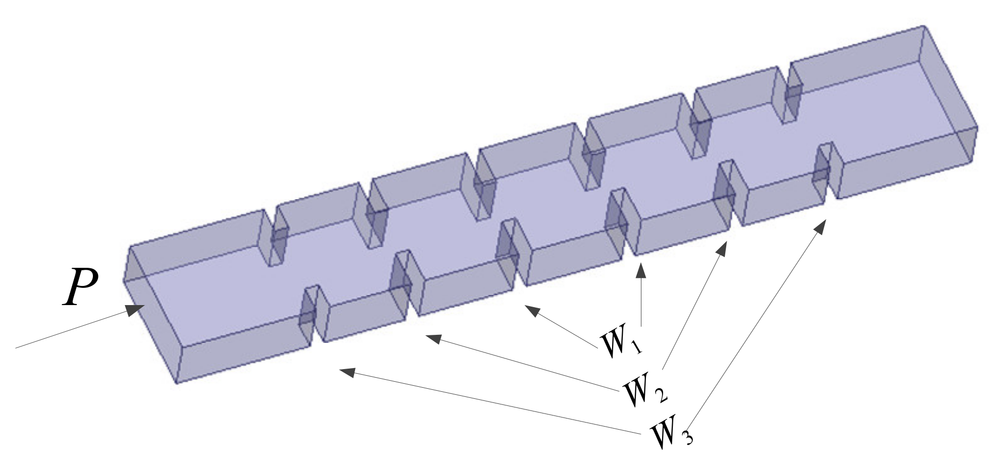
In the first example, the proposed modeling technique is applied to the iris coupled microwave cavity filter, as shown in Figure 3. The filter structure is a standard WR-90 waveguide (the width is 22.86 mm, and the height is 10.16 mm), and the thickness of all coupling windows is 2.54 mm. The iris widths $W_1$, $W_2$ and $W_3$ are the geometrical design parameters of the filter. The power P, which is supplied to the cavity filter, is a multiphysics design parameter. The power loss generates heat in the cavity, resulting in the thermal effects and mechanical deformation. These changes caused by thermal effects and mechanical deformation make the output of multiphysics simulation different from that of pure electromagnetic simulation. This example has four design parameters, i.e., $x={[W_1 W_2 W_3 P]}^T$. Frequency f is an extra input. The geometrical design parameter of the multiphysics model is $x_g={[W_1 W_2 W_3]}^T$. The multiphysics design parameter is $x_m=P$. The model has one output which represents the EM-centric multiphysics responses with respect to different values of multiphysics domain parameters, i.e., $y=S_{11}$. Only EM domain variables need to be considered for developing the coarse model. The coarse model has three design parameters $x_c={[W_1 W_2 W_3]}^T$. Frequency $f_c$ is an additional input.

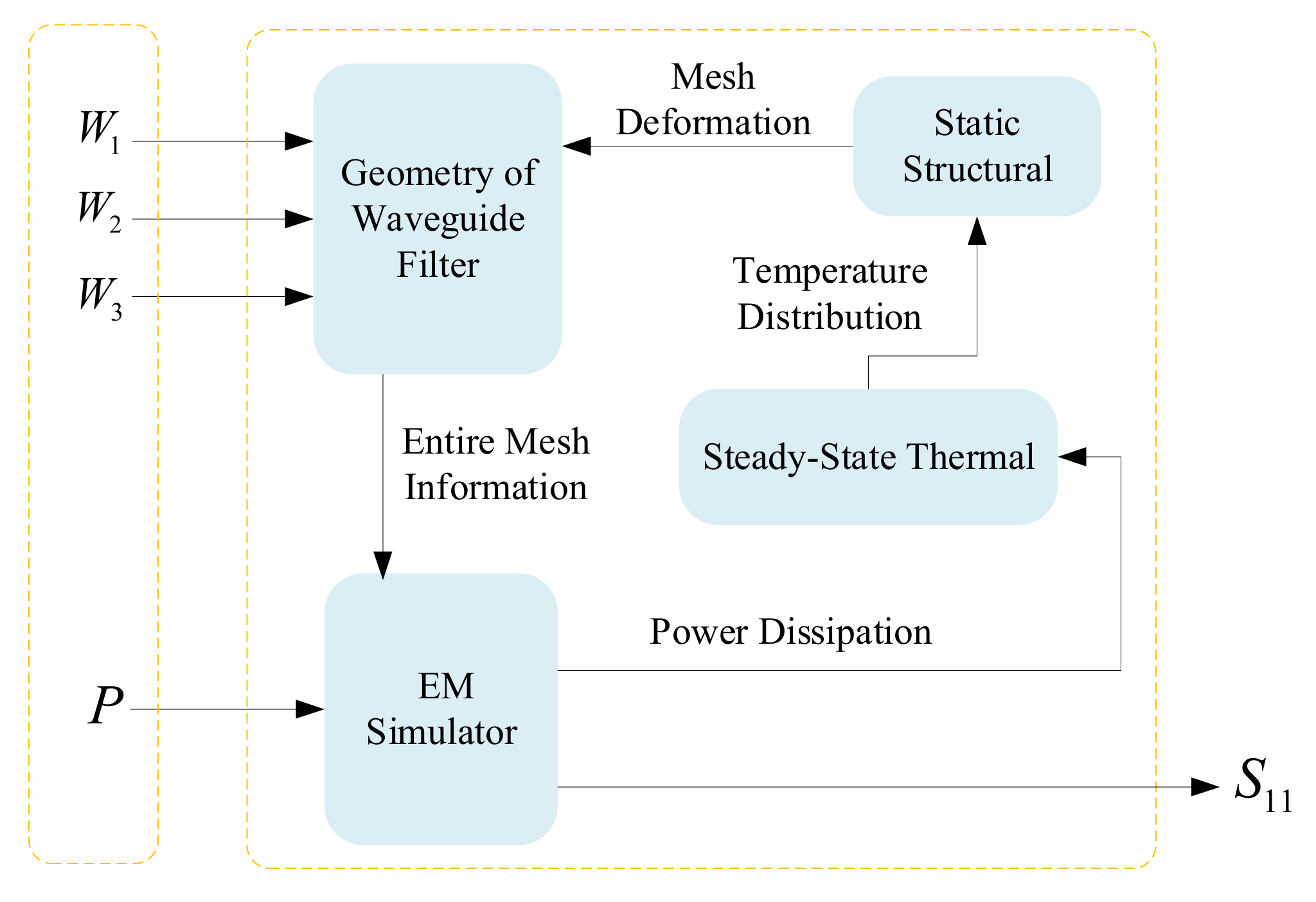
ANSYS Workbench 17.0 is used to perform multiphysics simulations to generate training and test samples for the multiphysics model. In this example, the interaction of three physics domains (thermal, mechanical and EM domain) leads to changes in EM responses. The actual simulation process of the ANSYS Workbench is shown in Figure 4. The geometry parameters of the waveguide filter perform EM simulation. The power loss generates heat with the action of the input power in the cavity filter, resulting in thermal deformation of the filter structure. Different physical domains interact with each other, and different input powers have different EM responses. Thus, more than simple electromagnetic field analysis is needed to represent multiple physical responses, and other physical domains need to be included in the model for multiple physical analysis. An ANSYS HFSS EM simulator with fast simulation capabilities generates data for the coarse model modeling. 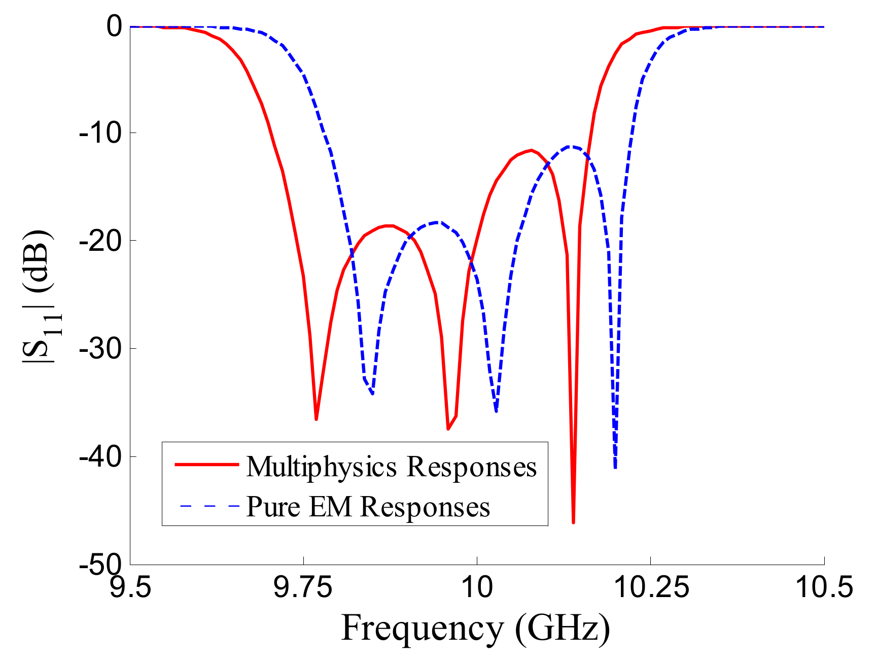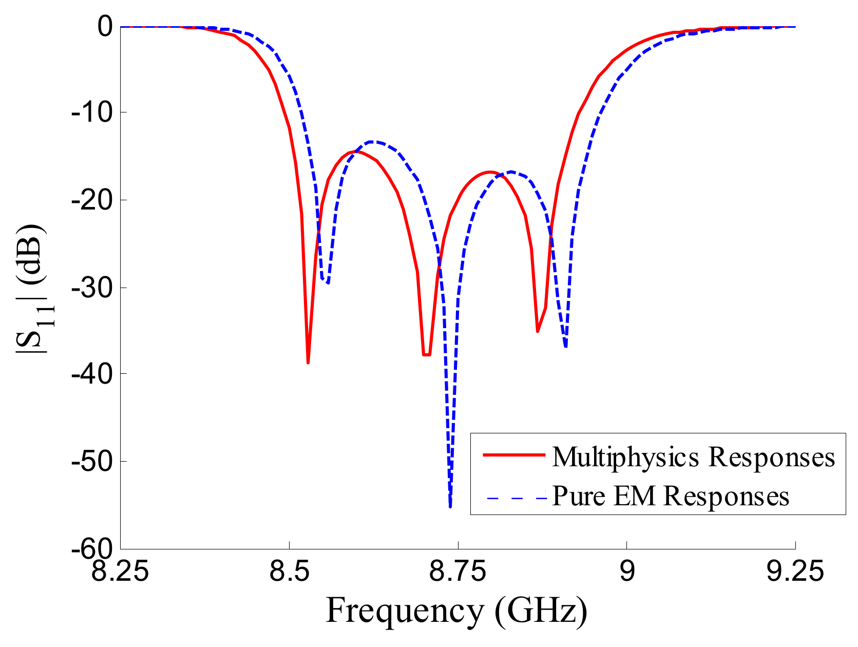Figure 5 shows the responses of EM analysis and multiphysics analysis with the same geometrical parameters. It is observed that there is a difference between multiphysics analysis and EM analysis with the same geometrical parameters, and the pure EM analysis cannot represent the multiphysics responses. In this paper, the proposed technique is developed to represent multiphysics responses for this filter example.

The DOE sampling method is utilized for data generation of the coarse model and the fine model. For the fine model, this example uses 5-level (25 sets) and 9-level (81 sets) of DOE to define multiphysics training data, respectively. The 8-level (64 sets) of DOE is used to define multiphysics test data. For the coarse model, 9-level (81 sets) of DOE is used to define EM domain training data; the 8-level (64 sets) of DOE is used to define EM domain test data. The test data are never used in the training process. To accurately map multiphysics problems to EM problems, the range of geometrical parameters of the coarse model is lager than that of the fine model.

Table 1. Definition of training and test data for multiphysics parametric modeling of the iris coupled microwave cavity filter.

Input Variables		Training Data			Test Data
		Min	Max	Step	Min	Max	Step
Coarse model	$W_1$ (mm)	4.81	5.13	0.04	4.83	5.11	0.04
	$W_2$ (mm)	6.73	7.05	0.04	6.75	7.03	0.04
	$W_3$ (mm)	7.24	7.56	0.04	7.26	7.54	0.04
Fine model	$W_1$ (mm)	4.818	5.098	0.07	4.84	5.085	0.035
	$W_2$ (mm)	6.7635	7.0035	0.06	6.792	7.002	0.03
	$W_3$ (mm)	7.254	7.494	0.06	7.285	7.495	0.03
	$P$ (W)	10	50	10	12.5	47.5	5

shows the ranges of the training and test data chosen in this example. The input frequency range is from 9.5 to 10.5 GHz with 0.01 GHz step. For this example, 8181 samples and 2525 samples are used to train the fine model, respectively, and 6464 samples are used to test the fine model. A total of 8181 samples are used to train the coarse model, and 6464 samples are used to test the coarse model. The training samples and test samples are imported into the software NeuroModelerPlus to complete the training and test process.

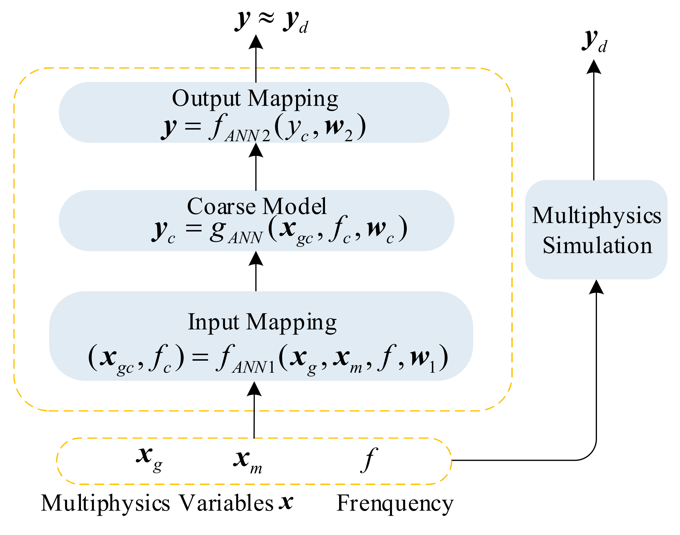
Before developing the multiphysics domain fine model, a four-layer multilayer perceptron (MLP) structure is used to develop the coarse model in this example. The training and test process of the coarse model is completed in NeuroModelerPlus. The numbers of hidden neurons in the two hidden layers of the coarse model are 10 and 10, respectively. After the establishment of the coarse model, the fine model, including two mapping neural networks and the trained coarse model, is developed. The construction and training process for the proposed multiphysics models is completed in NeuroModelerPlus, as well. The developed multiphysics model can represent the EM-centric multiphysics responses with respect to different values of multiphysics domain design parameters. The accuracy of the proposed model can be expressed by training error and test error, which are obtained by Equation (6). The training error for the developed multiphysics model with 81 sets of training data is 1.18%, while the test error is 1.22%. The numbers of hidden neurons for the input and output mapping are 10 and 10, respectively. The training error for the developed multiphysics model with 25 sets of training data is 1.20%, while the test error is 1.31%. The numbers of hidden neurons for the input and output mapping modules are 5 and 5, respectively. The development process of the multiphysics model takes about 15 min.

For this example, the ANN multiphysics modeling method in [17], the Neuro-TF multiphysics modeling method in [20] and the existing Neuro-SM multiphysics modeling method in [21] are used to develop the multiphysics model in two cases: with 25 sets of multiphysics training data and 81 sets of multiphysics training data. The coarse model and the numbers of hidden neurons of the multiphysics model in [21] are all the same as the proposed multiphysics model. The modeling results of four different modeling methods are compared from three aspects: the amount of modeling data, the modeling time and the modeling error, as shown in

Table 2. Modeling results of four multiphysics parametric modeling methods for the iris coupled microwave cavity filter.

Modeling Method	EM Data	Multiphysics Data	Training Error	Test Error	Training Time	Modeling Time
ANN model	0	81	1.81%	2.75%	0.1 h	10.6 h
		25	1.45%	14.76%	0.1 h	3.4 h
Neuro-TF model	0	81	1.49%	2.04%	0.25 h	10.75 h
		25	1.24%	3.14%	0.25 h	3.55 h
Existing Neuro-SM model	81	81	1.35%	1.85%	0.25 h	11.54 h
		25	1.43%	2.65%	0.25 h	4.34 h
Proposed Neuro-SM model	81	81	1.12%	1.23%	0.25 h	11.54 h
		25	1.20%	1.31%	0.25 h	4.34 h

.

The results in Table 2 show that the proposed model, which includes three modules, is more accurate than other models developed by the existing methods. The training error and the test error of the proposed model with less multiphysics data (25 sets) is much smaller than that of the ANN model with more multiphysics data (81 sets). Since the proposed model contains a coarse model which provides physical properties, the proposed model with less data and modeling time is more accurate than the ANN model. The output mapping is introduced into the proposed model to narrow the difference between the coarse model and the fine model. Therefore, the proposed model is more accurate than the Neuro-TF model and the existing Neuro-SM model with the same multiphysics data and modeling cost.

The comparison of computation time between ANSYS Workbench software and the proposed multiphysics model with respect to different amounts of multiphysics data is shown in

Table 3. Comparison of computation time between the multiphysics software simulation and the proposed Neuro-SM multiphysics model (25 data) for the iris coupled microwave cavity filter.

No. of Multiphysics Data	Computation Time
	ANSYS Workbench	Proposed Neuro-SM Model
1	≈7 min	4.34 h + 0.03 s
50	≈6 h	4.34 h + 1.6 s
100	≈12 h	4.34 h + 3.1 s

. It can be seen from the table that the multiphysics simulation software (ANSYS Workbench) takes a lot of time to calculate new multiphysics data. However, the modeling cost and time of the proposed model is a one-time investment. Once the proposed model is established, the time to calculate new multiphysics data is negligible. The advantage of the proposed multiphysics is more obvious with more calculated data.

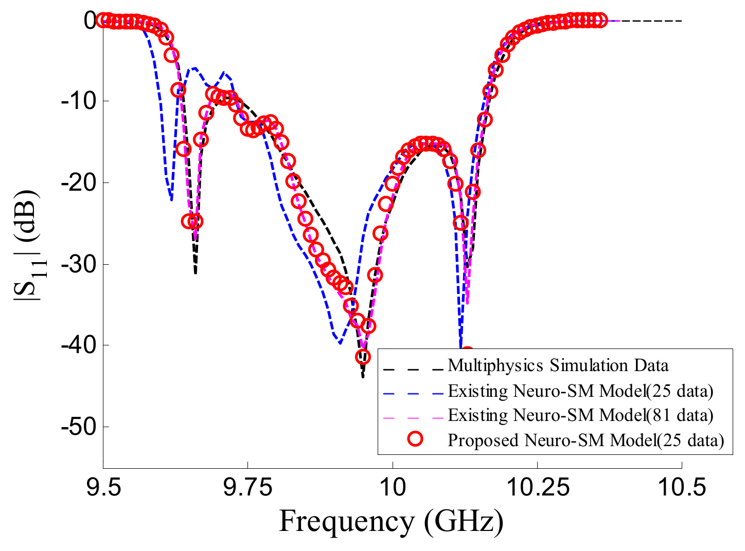
The comparison of the decibel values of $S_{11}$ of the proposed multiphysics model trained with less data (25 sets) and the existing Neuro-SM model trained with less (25 sets) and more data (81 sets) are shown in Figure 6. The four models are operated under the same design parameters randomly selected from the test data. The proposed multiphysics model can provide accurate prediction for the test sample even if it has never been learned in the training process. Compared with the existing Neuro-SM model, the proposed model can achieve better accuracy.

3.2. Three-Pole Waveguide Filter

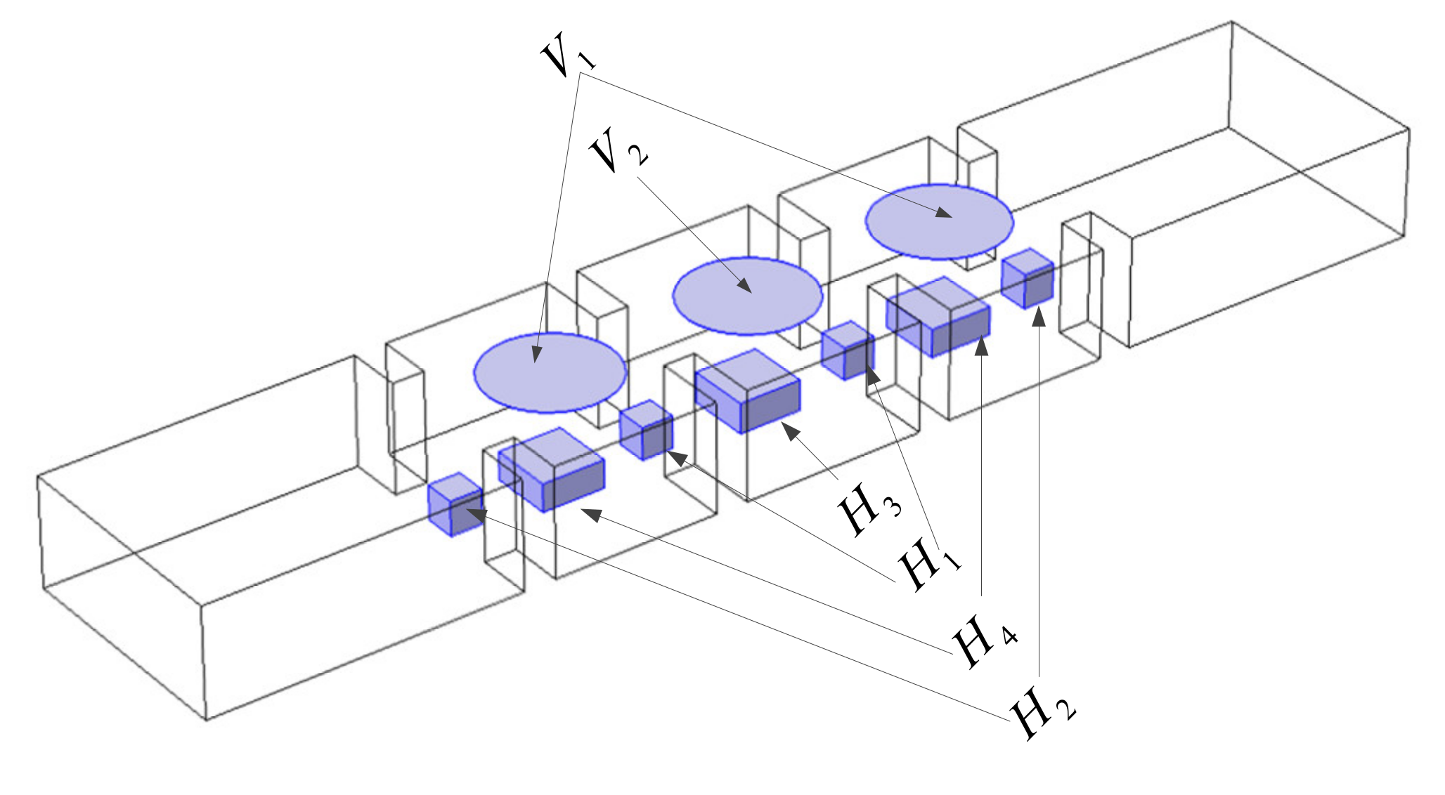
For the second example, the proposed parametric modeling technique is applied to a three-pole waveguide filter with tuning posts placed at the center of each coupling window and cavity, as shown in Figure 7. The heights of the tuning posts ($H_1$ and $H_2$) and the square cross section ($H_3$ and $H_4$) are the geometrical design parameters of this filter. The electronic potentials $V_1$ and $V_2$ applied across the piezo-actuator are multiphysics design parameters, which provide the tunability for the waveguide filter by causing the deformation of the piezo-actuator. The multiphysics design parameters $V_1$ and $V_2$ can change the EM response due to the piezoelectric effect and mechanical deformation. The waveguide structure is a standard WR-90 waveguide (the width is 22.86 mm and the height is 10.16 mm), and the thickness of all coupling windows is 3 mm. This example has six design parameters, i.e., $x={[H_1 H_2 H_3 H_4 V_1 V_2]}^T$. Frequency $f$ is an extra input. The geometrical design parameter of the multiphysics model is $x_g={[H_1 H_2 H_3 H_4]}^T$; the multiphysics design parameter is $x_m={[V_1 V_2]}^T$. The model has one output which represents the EM-centric multiphysics responses with respect to different values of multiphysics domain design parameters, i.e., $y=S_{11}$. Only EM domain variables need to be considered for developing the coarse model. The geometrical design parameter of the coarse model is $x_c={[H_1 H_2 H_3 H_4]}^T$. Frequency $f_c$ is an additional input of the coarse model.

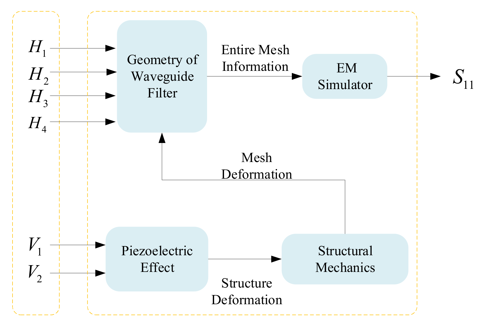
In this example, training and test samples for the multiphysics model are generated by COMSOL Multiphysics 5.3a, which performs multiphysics simulations. The interaction of three physics domains (electrostatic, mechanical and EM domain) leads to the changes in EM responses. The actual simulation process of COMSOL Multiphysics is shown in Figure 8. The geometry parameters of the waveguide filter perform EM simulation. The variation in the bias voltage $V_1$ and $V_2$, which causes the deformation of the piezoelectric actuator, can change the EM response. Different $V_1$ and $V_2$ have different response waveforms, thus, the bias voltages $V_1$ and $V_2$ need to be included in the multiphysical model. The ANSYS HFSS EM simulator with fast simulation capabilities generates modeling data for the coarse model modeling. Figure 9 shows the responses of EM analysis and multiphysics analysis with the same geometrical parameters. It is observed that there is a difference between multiphysics analysis and EM analysis with the same geometrical parameters. Pure EM analysis cannot represent the multiphysics responses. In this paper, the proposed technique is developed to represent multiphysics responses for this filter example.

DOE sampling method is utilized for data generation of the coarse model and the fine model. For the fine model, this example uses 5-level (25 sets) and 9-level (81 sets) of DOE to define multiphysics training data, respectively. The 8-level (64 sets) of DOE is used to define multiphysics test data. For the coarse model, 9-level (81 sets) of DOE is used to define EM domain training data, and 8-level (64 sets) of DOE is used to define EM domain test data. The test data are never used in the training process. To accurately map multiphysics problems to EM problems, the range of geometrical parameters of the coarse model is larger than that of the fine model.

Table 4. Definition of training and test data for multiphysics parametric modeling of the three-pole waveguide filter.

Input Variables		Training Data			Test Data
		Min	Max	Step	Min	Max	Step
Coarse model	$H_1$ (mm)	2.86	3.1	0.03	2.87	3.08	0.03
	$H_2$ (mm)	3.08	3.32	0.03	3.09	3.30	0.03
	$H_3$ (mm)	2.73	2.97	0.03	2.74	2.95	0.03
	$H_4$ (mm)	2.535	2.775	0.03	2.54	2.75	0.03
Fine model	$H_1$ (mm)	2.875	3.075	0.05	2.89	3.065	0.025
	$H_2$ (mm)	3.1	3.3	0.05	3.115	3.29	0.025
	$H_3$ (mm)	2.75	2.95	0.05	2.765	2.94	0.025
	$H_4$ (mm)	2.55	2.75	0.05	2.565	2.74	0.025
	$V_1$ (V)	−400	400	100	−175	175	50
	$V_2$ (V)	−400	400	100	−175	175	50

shows the ranges of the training and test data chosen in this example. The input frequency range is from 8.25 to 9.25 GHz with 0.01 GHz step. For this example, 8181 samples and 2525 samples are used to train the fine model, respectively, and 6464 samples are used to test the fine model. In all, 8181 samples are used to train the coarse model, and 6464 samples are used to test the coarse model. The training samples and test samples are imported into the NeuroModelerPlus software to complete the training and test process.

Before developing the multiphysics domain fine model, a three-layer MLP structure is used to develop the coarse model in this example. The training and test process for the coarse model is completed in NeuroModelerPlus. The numbers of hidden neurons for the coarse model are 30 and 20 when 25 and 81 sets of training data are used to develop the multiphysics fine model, respectively. After the establishment of the coarse model, the fine model, including two mapping neural networks and the trained coarse model, is developed. The construction and training process of the proposed multiphysics model is completed in NeuroModelerPlus, as well. The developed multiphysics model can represent the EM-centric multiphysics responses with respect to different values of multiphysics domain design parameters. The accuracy of the proposed model can be expressed by training error and test error, which are obtained by Equation (6). The training error for the developed multiphysics model with 81 sets of training data is 1.19%, while the test error is 1.24%. The numbers of hidden neurons for the input and output mapping are 5 and 5, respectively. The training error for the developed multiphysics model with 25 sets of training data is 1.25%, while the test error is 1.63%. The numbers of hidden neurons of the input and output mapping are the same as the numbers for 81 sets of training data. The development process of multiphysics model takes about 18 min.

For this waveguide filter example, the ANN multiphysics modeling method in [17], the Neuro-TF multiphysics modeling method in [20] and the existing Neuro-SM multiphysics modeling method in [21] are used to develop the multiphysics model in two cases: with 25 sets of multiphysics training data and 81 sets of multiphysics training data. The coarse model and the numbers of hidden neurons of the multiphysics model in [21] are the same as the proposed multiphysics model. The modeling results of four different modeling methods are compared from three aspects: the amount of modeling data, the modeling time and the modeling error, as shown in

Table 5. Modeling results of four multiphysics parametric modeling methods for the three-pole waveguide filter.

Modeling Method	EM data	Multiphysics Data	Training Error	Test Error	Data Generation Time	Training Time	Modeling Time
ANN model	0	81	1.35%	2.94%	67.9 h	0.15 h	68.05 h
		25	1.30%	13.22%	23.5 h	0.15 h	23.65 h
Neuro-TF model	0	81	1.53%	2.34%	67.9 h	0.15 h	68.05 h
		25	1.29%	4.21%	23.5 h	0.15 h	23.65 h
Existing Neuro-SM model	81	81	1.58%	1.71%	69.2 h	0.3 h	69.5 h
		25	1.61%	2.50%	24.8 h	0.3 h	25.1 h
Proposed Neuro-SM model	81	81	1.19%	1.44%	69.2 h	0.3 h	69.5 h
		25	1.25%	1.63%	24.8 h	0.3 h	25.1 h

. The results in Table 5 show that the proposed model, which includes three modules, is more accurate than other models developed by the existing methods. The training error and the test error of the proposed model with less multiphysics data (25 sets) is much smaller than that of the ANN model with more multiphysics data (81 sets). Since the proposed model contains a coarse model which provide physical properties, the proposed model with less data and modeling time is more accurate than the ANN model. The output mapping is introduced into the proposed model to narrow the difference between the coarse model and the fine model. Therefore, the proposed model is more accurate than the Neuro-TF model and the existing Neuro-SM model with the same multiphysics data and modeling cost.

The comparison of computation time between COMSOL Multiphysics software and the proposed multiphysics model with respect to different amounts of multiphysics data are shown in

Table 6. Comparison of computation time between the multiphysics software simulation and the proposed Neuro-SM multiphysics model (25 data points) for the three-pole waveguide filter.

No. of Multiphysics Data	Computation Time
	COMSOL Multiphysics	Proposed Neuro-SM Model
1	$\approx$0.9 h	25.1 h + 0.05 s
50	$\approx$45 h	25.1 h + 2 s
100	$\approx$90 h	25.1 h + 4 s

. It can be seen from the table that the multiphysics simulation software (COMSOL Multiphysics) requires a lot of time to calculate new multiphysics data. However, the modeling cost and time of the proposed model is a one-time investment. Once the proposed model is established, the time to calculate new multiphysics data is negligible. The advantage of the proposed multiphysics is more obvious with more calculated data.

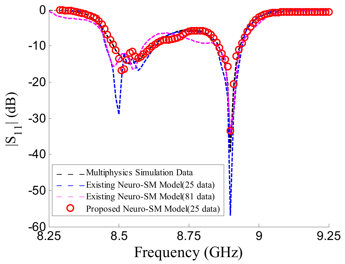
The comparison of the decibel values of S₁₁ of the proposed multiphysics model trained with less data (25 sets) and the existing Neuro-SM model trained with less (25 sets) and more data (81 sets) are shown in Figure 10. The four models are operated under the same design parameters randomly selected from the test data. The proposed multiphysics model can provide an accurate prediction for test samples even if it has never been learned in the training process. Compared with the existing Neuro-SM model, the proposed model can achieve better accuracy.

4. Conclusions

This paper proposed an advanced Neuro-SM multiphysics parametric modeling approach for microwave passive components. The output mapping is introduced into the Neuro-SM multiphysics model for the first time to match the coarse model output with the multiphysics data. The proposed technique provides more effective combinations between the mapping structure and the coarse model. A three-stage training method is proposed to accurately develop the proposed multiphysics model. The proposed model can achieve good accuracy using less multiphysics data than the existing Neuro-SM model, the Neuro-TF model and the ANN model. Compared with the multiphysics software simulation, the developed multiphysics model can provide an accurate prediction of EM-centric multiphysics responses using less computational time and less computational cost. The more multi-physical responses required, the more obvious the advantage of the proposed model in time consumption. The proposed parametric modeling technique shortens the design cycle time and improves the design accuracy. The two microwave filter examples verify the applicability and advantage of the proposed technique.