Communication

Experimental Detection of Initial System–Environment Entanglement in Open Systems

Beijing Computational Science Research Center, Beijing 100084, China
*
Author to whom correspondence should be addressed.
Photonics 2022, 9(11), 883; https://doi.org/10.3390/photonics9110883
Submission received: 25 October 2022 / Revised: 15 November 2022 / Accepted: 16 November 2022 / Published: 21 November 2022
(This article belongs to the Section Quantum Photonics and Technologies)

Abstract

:
We experimentally investigate how initial entanglement between the system and environment can be detected in an open system by using some prior knowledge of the joint evolutions. The protocol we employed requires classical optimization on the results after performing measurements on the system state. Such an approach does not require a full 2-qubit QST, and works in scenarios where one has access to the system only. We demonstrate the protocol on both pure entangled states and mixed entangled states. The obtained results show the experimental accessibility and validity of the protocol. Compared with the previous methods, which also assume access only to the system, this protocol is less demanding in terms of measurement and state preparation. The experimental results also show that, using the knowledge of the interaction, we can fine-tune the protocol, thus showing the potential of the protocol for developing experimentally feasible and practical entanglement detection methods.

1. Introduction

Quantum entanglement, a non-classical and counter-intuitive phenomena, is the core foundation of quantum mechanics. Quantum entanglement acts as a crucial resource in quantum information science. However, in some cases, unwanted initial system–environment entanglement can be a hindrance, which leads to errors in performing quantum information tasks. In the past two decades since Werner [1] formulated the definition of entanglement, great efforts have been devoted to entanglement detection, such as positive partial transpose criterion [2], entanglement witness [3,4,5,6,7,8,9,10,11], matrix realignment criterion (or computable cross norm criterion) [12,13], complementarity [14,15,16,17], etc. These methods assume that one has access to both parts of a bipartite system. However, in some cases, entanglement arises between a system and some other system that is inaccessible. Detecting these kinds of initial correlation is important for the application of error prevention methods [18]. In recent years, important methods have been proposed [19,20,21,22,23,24,25,26,27] and experimentally demonstrated [28,29,30], which show the possibility of witnessing system–environment entanglement by measurements performed in open systems alone.
In Ref. [31], the authors address the problem of how initial system–environment correlation can be verified by monitoring system evolution alone if one makes the experimentally reasonable assumption that the system–environment interaction is known. Their results can be applied in experimental quantum control and quantum computing where the system and environment are often assumed to be initially uncorrelated. This theory is then developed for practical use and considered with the experimentally relevant Hamiltonian [32]. It differs from previous methods [21,22,23,24,25,26] in that it does not require the preparation of different initial states. In addition, it requires less measurement resource than the method in [19].
In this article, we report an experimental detection of initial system–environment entanglement by measuring the system alone. Such a method rests on prior knowledge of the cause of the system–environment interaction but assumes nothing of the environment state. It is suitable for a scenario where full 2-qubit quantum state tomography (QST) is not available or access to the environment is prohibited, and the only resource provided is measurements on the system. We test the performance of the protocol on both pure entangled states and mixed entangled states. Our experimental results show validity of the method for verification of initial system–environment entanglement, and further provides a practical test bed for entanglement detection.

2. Detecting Initial Entanglement in Open Systems

The dynamics of a closed quantum system is characterized by a unitary transformation. However, for an open system—that is, when the system interacts with some external environment—its dynamics is non-unitary. For an open system (S), which is initialized (at time t 0 ) in a composite state ρ S E with the environment (E), the dynamics is formulated as follows: let the system and environment evolve together unitarily, and then trace over the environment at some time t. Mathematically, the reduced dynamics of the system can be written as
ρ S ( t 0 ) ρ S ( t ) = Tr E { U S E ρ S E ( t 0 ) U S E } ,
where ρ S ( ρ S ) is the initial (final) state of the system.
We consider a scenario where for many identical preparations of ρ S E , we have only access to the system and QST is used to reconstruct the density matrix of ρ S and ρ S . Given an initial state ρ S E , we check whether the reduced-state dynamics map (1), ρ S ρ S , can be obtained by assuming an initially uncorrelated state ρ S E * = ρ S ρ E * and, thus, determine whether there exists initial entanglement in ρ S E . Apparently, if no such ρ S E * permits the reconstruction of the map (1), the system and the environment must be initially correlated in ρ S E . We make no assumptions about the environment state ρ E * , and just assume that the system and environment consist of two qubits and are in the form of a direct product state. The environment can be any valid qubit-state, which can be represented as follows:
ρ E * = 1 2 ( I + x σ X + y σ X + z σ Z ) ,
where σ X ( Y , Z ) are Pauli operators; x , y , z are real parameters and satisfy x 2 + y 2 + z 2 1 . Then, we calculate the final state of ρ S E * after the transformation under U SE and obtain the reduced final state ρ S * = Tr E { U S E ρ S E * ( t 0 ) U S E } of the system.
What we care about is whether this hypothetical reduced-state dynamics ρ S ρ S * is the same as that of (1). We define D to measure the distance between ρ S and ρ S * , which takes the form
D = min x , y , z | Δ ρ i j | 2 1 / 2
with x 2 + y 2 + z 2 1 and Δ ρ ρ S ρ S * .
In summary, for a given bipartite state ρ S E , the procedure to detect initial entanglement between the system and environment is as follows: (i) Perform QST on the initial state of the system to construct the form of the density matrix. (ii) Let the system–environment state ρ S E evolve under the coupling U S E . Then, perform QST to reconstruct the density matrix of the system’s final state to monitor its reduced evolution ρ S ρ S . (iii) Evaluate the distance D. Here, a classical optimization process over the parameters { x , y , z } is required to obtain the value of D. If it ends up with a non-zero value, then the hypothetical effort to reconstruct the map (1) by assuming a initially separable state ρ S E * = ρ S ρ E * fails, and initial entanglement between the system and environment is identified. Otherwise, if D = 0 , no initial entanglement is experimentally identified, but the existence of initial entanglement cannot be ruled out. We provide analyses later for when we can state with certainty that there are initial entanglements by measuring S only, with the knowledge of U S E . Then, we can fine-tune the parameter τ and, thus, strengthen the performance of the protocol.
Initial system–environment correlation cannot be credibly determined by measuring the system separately, if one has no prior knowledge of system–environment dynamics [31]. From the viewpoint of practical application, we consider the Heisenberg interaction, which is an experimentally relevant Hamiltonian:
H ex = J ( σ X σ X + σ Y σ Y + σ Z σ Z ) ,
with J being a coupling constant. Its corresponding time evolution operator e i H ex t is given by
U ( τ ) = e i τ 0 0 0 0 e i τ cos 2 τ i e i τ sin 2 τ 0 0 i e i τ sin 2 τ e i τ cos 2 τ 0 0 0 0 e i τ .
Here, we use the term τ = J t for simplicity.
Using the prior knowledge of interaction, we experimentally demonstrate the above method for certifying initial system–environment entanglement through measuring the system state alone, with single photons and linear optical setup.

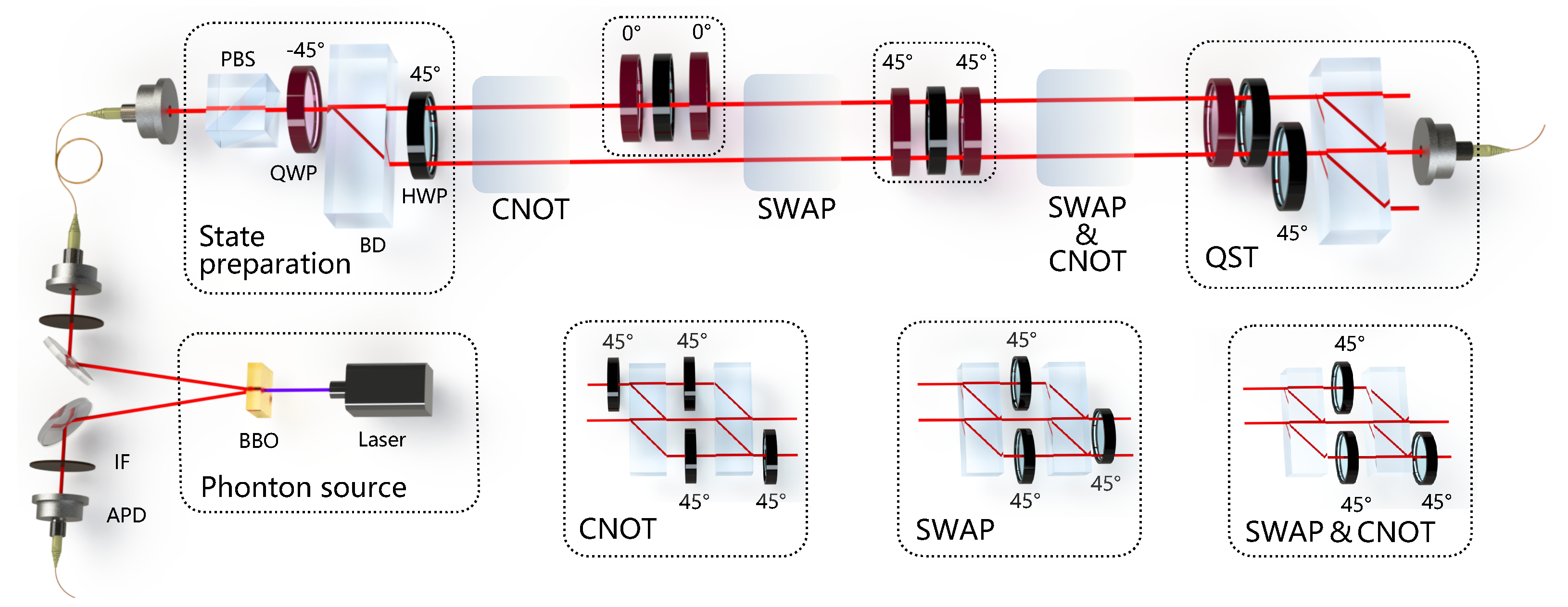
3. Experimental Demonstration

The experimental setup is illustrated in Figure 1. Pairs of photons used in this experiment are produced via a type-I spontaneous parametric down-conversion technique by pumping a β -barium-borate (BBO) with a 405 nm laser diode. With the detection of trigger photons, the other photons in one pair are heralded and act as a single photon source. Experimentally, this trigger–herald pair is counted by coincidences of two single-photon avalanche photodiodes (APDs). Total coincidence counts are about 11,000 over a collection time of 1 s within a 3 ns time window.
The heralded photons are polarized by passing through a polarizing beam splitter (PBS). Then, a quarter-wave plate (QWP) with setting angles θ Q P is inserted to rotate the polarizations of the photons.
In the experiment, we test the performance of the method carried out on maximally entangled states and two types of mixed entangled states. The polarizations of photons are encoded as the system qubit: { H = 0 p , V = 1 p } (H (V) represents the horizontal (vertical) polarization; the subscripts p refer to the “polarization” modes). Then, a birefringent calcite beam displacer (BD) is inserted to introduce two spatial modes. A BD directly transmits vertically polarized photons and laterally deflects horizontally polarized photons into upper (U) and lower modes (D), respectively, which are encoded as the environment qubit { D = 0 s , U = 1 s } (the subscripts s refer to the “spatial” modes). A half-wave plate (HWP) at 45 is placed to flip the polarizations between V to H , which is required for state preparation. The operation of an HWP with setting angle θ can be expressed in the matrix form as cos 2 θ sin 2 θ sin 2 θ cos 2 θ , and that of a QWP at ϑ can be expressed as cos 2 ϑ + i sin 2 ϑ ( 1 i ) sin ϑ cos ϑ ( 1 i ) sin ϑ cos ϑ sin 2 ϑ + i cos 2 ϑ .
By setting θ Q P at 45 , the composite polarization–spatial system is generated into a maximally entangled state, Φ ps = 1 2 ( 01 ps + i 10 ps ) , with a state-preparation fidelity higher than 99 % . The fidelity of the theoretical density ρ th and the experimental one ρ exp is defined [33] by F ( ρ th , ρ exp ) = ( Tr ρ th ρ exp ρ th ) 2 , which can be evaluated after construction of the density matrix via a full 2-qubit QST on the initial state.
The operation U ( τ ) (Equation (5)) can be decomposed into experimentally feasible operations controlled by two-qubit operation ( U ˜ ( τ ) ) and CNOT operation ( U CNOT ):
U ( τ ) = U CNOT U ˜ ( τ ) U CNOT ,
where U CNOT = U CNOT = I 0 0 σ X , and
U ˜ ( τ ) = U CNOT U ( τ ) U CNOT = e i τ 0 0 0 0 e i τ cos 2 τ 0 i e i τ sin 2 τ 0 0 e i τ 0 0 i e i τ sin 2 τ 0 e i τ cos 2 τ .
The CNOT operation is realized by two BDs and four HWPs at 45 as shown in Figure 1. The first BD splits the photons with different polarizations into different spatial modes and HWPs at 45 flip the polarization modes of the photons, followed by the second BD that combines two spatial modes back into one.
U ˜ ( τ ) can be further expanded as
U ˜ ( τ ) = ( I R Z ) ( I 0 0 s + R X 1 1 s ) ,
where R Z = e i τ σ Z and R X = e i 2 τ σ X R Y = e i 2 τ σ Y are qubit rotations. The controlled rotation in (8) is implemented by inserting a Q-H-Q wave-plate combination into the upper mode, with angles set at 0 , ( 180 τ / π ) and 0 , respectively, as shown in Figure 1. For the rotation R Z on the environment state (which is encoded by the spatial modes), we first apply a SWAP operation to transform the modes (between the spatial and polarization modes); then, we implement R Z on the polarization modes via inserting another Q-H-Q wave-plate combination, by rotating the HWP to ( 90 τ / π + 45 ) and fixing the other two QWPs at 45 . What follows is another SWAP operation that restores the mode transformation. This SWAP operation can be realized combined with the last CNOT operation to simplify the experimental implementation.
The last step is to estimate the evolved system state ρ S , which is realized via single-qubit QST. By means of projecting the output states into tomographic complete bases { H , V , ( H + V ) / 2 , ( H i V ) / 2 } , the density matrix of the output state can be obtained via maximum likelihood estimation. The projecting measurements are carried out by a sequence of a QWP, two HWPs and a BD, as shown in Figure 1. The resulting single photons are detected by avalanche photodiodes (APDs), in coincidence with the trigger photons.
To verify the validity of the method for experimentally detecting initial entanglement with access to the system alone, we also perform 2-qubit QST on the initial states ρ S E to directly determine the actual initial entanglement. Note that more measurement resources are required than the protocol. The entanglement measure we use here is concurrence [34,35], which can be evaluated with the measured density matrix from the 2-qubit QST. Concurrence varies between 0 and 1, indicating that the degree of entanglement changes from separable to maximally entangled. The measurement setup for the QST of the initial state is not illustrated in Figure 1.

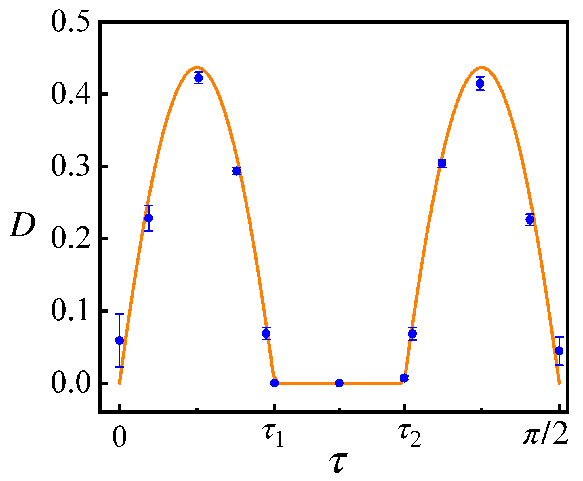
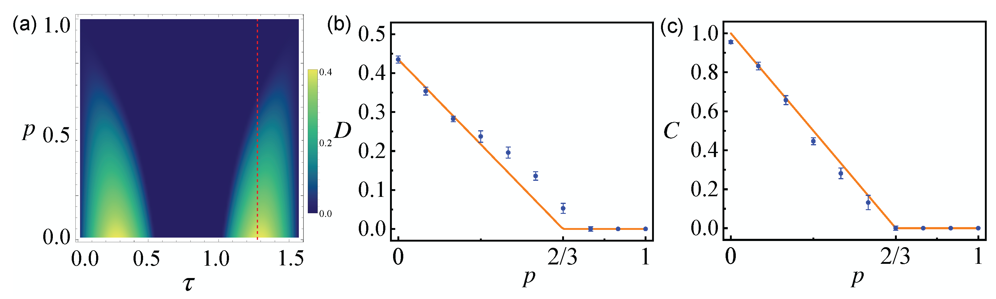
4. Results and Discussion

While initially preparing the maximally entangled state Φ ps , we experimentally investigate what values of τ enable us to detect initial entanglement by the protocol. In Figure 2, we show the experimental results (blue dots) and the theoretical predictions (yellow line) of the distance D versus τ . In a period of π 2 , except the interval when τ 2 > τ > τ 1 ( τ 1 = 1 2 arctan ( 2 ) + π 2 and τ 2 = 1 2 arctan ( 2 ) ), D is always non-zero, which indicates the failure of the hypothetical separable state model. In other words, there must be initial entanglement. Note that the relation of D versus τ is π 2 periodic.
In the following, we show the performance of the protocol for Werner states:
ρ S E = p 4 I I + ( 1 p ) Φ Φ ,
where 1 p 0 . The white noise in ρ S E is introduced in postprocessing. The probabilities p and 1 p are applied by evaluating the ratios of the measurement outcomes from two separated experiments for initial states Φ Φ ps and 1 4 I I ps . Figure 3a shows the numerical analysis of D (colored according to the degree of the distance D) dependence of p and τ . It can be seen that for different values of τ , the values of the measured D are different. Therefore, by varying τ , we can fine-tune the protocol for detecting entanglement of such a class of states (9).
Figure 3b shows the results obtained from performing the protocol. Through numerical analysis in Figure 3a, we select the optimal value τ = 13 32 π ; then, the protocol always enables detecting the initial entanglement for p < 2 / 3 , but not for values (of p) other than that, which is consistent with the reality of the entanglement (in concurrence measurement, see Figure 3c) of ρ S E , which is obtained from performing 2-qubit QST on ρ S E . To our surprise, the distance D also coincides with the monotonicity of C (Figure 3c). Compared with those QST-based methods, this protocol requires less measurement resources but achieves the same goal. In addition, it does not require access to the environment.
The experimental results are in good agreement with the theoretical predictions, and the slight differences are due to the experimental imperfection during the state-preparation stage and the measurement stage. Our results prove that the protocol is valid for detecting initial system–environment entanglement by only measuring the system. We want to stress that, although the U S E and the states we considered are motivated by realistic experimental conditions, the protocol can be further explored for other types of joint interactions and entangled states.

5. Conclusions

We have reported an experimental demonstration of a protocol for detecting initial system–environment entanglement by measuring the system alone. The protocol requires classical optimization based on the results after performing measurements on the system state. This approach works in scenarios where one only has access to the system and a full 2-qubit QST is not available. We test the performance of the protocol on both pure entangled states and mixed entangled states. The obtained results show the experimental accessibility and validity of the method. The advantage of the method is that it requires fewer measurements than conventional methods based on a full 2-qubit QST; compared with previous methods, which also assume access to the system alone, it is less demanding in terms of measurement and state preparation. We also experimentally show that, using the knowledge of U S E , we can fine-tune the protocol, thus demonstrating the potential for developing entanglement detecting methods for a wide range of states.

Author Contributions

Conceptualization, P.X.; methodology, P.X. and L.X.; investigation, D.Q.; writing—original draft preparation, G.Z.; writing—review and editing, P.X.; visualization, G.Z.; supervision, P.X. All authors have read and agreed to the published version of the manuscript.

Funding

This research was funded by the National Natural Science Foundation of China (Grant Nos. 12025401, 92265209 and 12104036).

Institutional Review Board Statement

Not applicable.

Informed Consent Statement

Not applicable.

Data Availability Statement

All data included in this study are available upon request by contact with the corresponding author.

Conflicts of Interest

The authors declare no conflict of interest.

References

  1. Werner, R.F. Quantum states with Einstein-Podolsky-Rosen correlations admitting a hidden-variable model. Phys. Rev. A 1989, 40, 4277–4281. [Google Scholar] [CrossRef] [PubMed]
  2. Peres, A. Separability Criterion for Density Matrices. Phys. Rev. Lett. 1996, 77, 1413–1415. [Google Scholar] [CrossRef] [PubMed] [Green Version]
  3. Horodecki, M.; Horodecki, P.; Horodecki, R. Separability of mixed states: Necessary and sufficient conditions. Phys. Lett. A 1996, 223, 1–8. [Google Scholar] [CrossRef] [Green Version]
  4. Terhal, B.M. Bell inequalities and the separability criterion. Phys. Lett. A 2000, 271, 319–326. [Google Scholar] [CrossRef] [Green Version]
  5. Terhal, B.M. A family of indecomposable positive linear maps based on entangled quantum states. Linear Algebra Appl. 2001, 323, 61–73. [Google Scholar] [CrossRef] [Green Version]
  6. Terhal, B.M. Detecting quantum entanglement. Theor. Comput. Sci. 2002, 287, 313–335. [Google Scholar] [CrossRef] [Green Version]
  7. Tóth, G.; Gühne, O. Detecting Genuine Multipartite Entanglement with Two Local Measurements. Phys. Rev. Lett. 2005, 94, 060501. [Google Scholar] [CrossRef] [Green Version]
  8. Bovino, F.A.; Castagnoli, G.; Ekert, A.; Horodecki, P.; Alves, C.M.; Sergienko, A.V. Direct Measurement of Nonlinear Properties of Bipartite Quantum States. Phys. Rev. Lett. 2005, 95, 240407. [Google Scholar] [CrossRef] [Green Version]
  9. Gühne, O.; Lütkenhaus, N. Nonlinear Entanglement Witnesses. Phys. Rev. Lett. 2006, 96, 170502. [Google Scholar] [CrossRef] [Green Version]
  10. Augusiak, R.; Demianowicz, M.; Horodecki, P. Universal observable detecting all two-qubit entanglement and determinant-based separability tests. Phys. Rev. A 2008, 77, 030301. [Google Scholar] [CrossRef]
  11. Zhu, G.; Zhang, C.; Wang, K.; Xiao, L.; Xue, P. Experimental witnessing for entangled states with limited local measurements. Photon. Res. 2022, 10, 2047–2055. [Google Scholar] [CrossRef]
  12. Rudolph, O. On the cross norm criterion for separability. J. Phys. A Math. Gen. 2003, 36, 5825. [Google Scholar] [CrossRef]
  13. Chen, K.; Wu, L.A. A matrix realignment method for recognizing entanglement. arXiv 2002, arXiv:quant-ph/0205017. [Google Scholar] [CrossRef]
  14. Maccone, L.; Bruß, D.; Macchiavello, C. Complementarity and Correlations. Phys. Rev. Lett. 2015, 114, 130401. [Google Scholar] [CrossRef] [PubMed] [Green Version]
  15. Qian, X.F.; Vamivakas, A.N.; Eberly, J.H. Entanglement limits duality and vice versa. Optica 2018, 5, 942–947. [Google Scholar] [CrossRef] [Green Version]
  16. Spengler, C.; Huber, M.; Brierley, S.; Adaktylos, T.; Hiesmayr, B.C. Entanglement detection via mutually unbiased bases. Phys. Rev. A 2012, 86, 022311. [Google Scholar] [CrossRef] [Green Version]
  17. Bian, Z.H.; Wu, H. Experimental Certification of Quantum Entanglement Based on the Classical Complementary Correlations of Two-Qubit States. Photonics 2021, 8, 525. [Google Scholar] [CrossRef]
  18. Viola, L.; Lloyd, S. Dynamical suppression of decoherence in two-state quantum systems. Phys. Rev. A 1998, 58, 2733–2744. [Google Scholar] [CrossRef] [Green Version]
  19. Modi, K. Operational approach to open dynamics and quantifying initial correlations. Sci. Rep. 2012, 2, 581. [Google Scholar] [CrossRef] [Green Version]
  20. Ringbauer, M.; Wood, C.J.; Modi, K.; Gilchrist, A.; White, A.G.; Fedrizzi, A. Characterizing Quantum Dynamics with Initial System-Environment Correlations. Phys. Rev. Lett. 2015, 114, 090402. [Google Scholar] [CrossRef]
  21. Laine, E.M.; Piilo, J.; Breuer, H.P. Witness for initial system-environment correlations in open-system dynamics. Europhys. Lett. 2011, 92, 60010. [Google Scholar] [CrossRef] [Green Version]
  22. Smirne, A.; Breuer, H.P.; Piilo, J.; Vacchini, B. Initial correlations in open-systems dynamics: The Jaynes-Cummings model. Phys. Rev. A 2010, 82, 062114. [Google Scholar] [CrossRef] [Green Version]
  23. Gessner, M.; Breuer, H.P. Detecting Nonclassical System-Environment Correlations by Local Operations. Phys. Rev. Lett. 2011, 107, 180402. [Google Scholar] [CrossRef] [PubMed]
  24. Dajka, J.; Łuczka, J.; Hänggi, P. Distance between quantum states in the presence of initial qubit-environment correlations: A comparative study. Phys. Rev. A 2011, 84, 032120. [Google Scholar] [CrossRef] [Green Version]
  25. Gessner, M.; Breuer, H.P. Local witness for bipartite quantum discord. Phys. Rev. A 2013, 87, 042107. [Google Scholar] [CrossRef] [Green Version]
  26. Wißmann, S.; Leggio, B.; Breuer, H.P. Detecting initial system-environment correlations: Performance of various distance measures for quantum states. Phys. Rev. A 2013, 88, 022108. [Google Scholar] [CrossRef] [Green Version]
  27. Zhan, X. Determining the mixed high-dimensional Bell state of a photon pair through the measurement of a single photon. Phys. Rev. A 2021, 103, 032437. [Google Scholar] [CrossRef]
  28. Li, C.F.; Tang, J.S.; Li, Y.L.; Guo, G.C. Experimentally witnessing the initial correlation between an open quantum system and its environment. Phys. Rev. A 2011, 83, 064102. [Google Scholar] [CrossRef]
  29. Smirne, A.; Brivio, D.; Cialdi, S.; Vacchini, B.; Paris, M.G.A. Experimental investigation of initial system-environment correlations via trace-distance evolution. Phys. Rev. A 2011, 84, 032112. [Google Scholar] [CrossRef] [Green Version]
  30. Gessner, M.; Ramm, M.; Pruttivarasin, T.; Buchleitner, A.; Breuer, H.P.; Häffner, H. Local detection of quantum correlations with a single trapped ion. Nat. Phys. 2014, 10, 105–109. [Google Scholar] [CrossRef]
  31. Chitambar, E.; Abu-Nada, A.; Ceballos, R.; Byrd, M. Restrictions on initial system-environment correlations based on the dynamics of an open quantum system. Phys. Rev. A 2015, 92, 052110. [Google Scholar] [CrossRef]
  32. Hagen, S.; Byrd, M. Detecting initial system-environment correlations in open systems. Phys. Rev. A 2021, 104, 042406. [Google Scholar] [CrossRef]
  33. Jozsa, R. Fidelity for Mixed Quantum States. J. Mod. Opt. 1994, 41, 2315–2323. [Google Scholar] [CrossRef]
  34. Hill, S.A.; Wootters, W.K. Entanglement of a Pair of Quantum Bits. Phys. Rev. Lett. 1997, 78, 5022–5025. [Google Scholar] [CrossRef] [Green Version]
  35. Wootters, W.K. Entanglement of Formation of an Arbitrary State of Two Qubits. Phys. Rev. Lett. 1998, 80, 2245–2248. [Google Scholar] [CrossRef]
Figure 1. Photon pairs are produced via type-I spontaneous parametric down-conversion process by pumping a 1 mm-thick BBO nonlinear crystal with a 405 nm laser diode. Two IFs filter out the pump and restrict the photon bandwidth to 3 nm. The operations (CNOT and SWAP) are realized with combinations of BDs and HWPs at 45 . The system qubit is polarization analyzed via a QST module consisting of a QWP and two HWPs followed by a BD in front of an APD. Coincidence measurements are performed via APDs. BD, beam displacer; HWP, half-wave plates; QWP, quarter-wave plate; PBS, polarizing beam splitter; IF, interference filter; BBO, β -barium-borate; APD, avalanche photodiodes.
Photonics 09 00883 g001
Figure 2. The defined distance D as a function of the evolution time parameter τ for the maximally entangled state. Outside the interval τ 2 > τ > τ 1 (with τ 1 = 1 2 arctan ( 2 ) + π 2 and τ 2 = 1 2 arctan ( 2 ) ), the measured D is always non-zero, indicating the presence of entanglement in the initial state ρ S E . The solid orange curve indicates the theoretical predictions and the blue symbols denote the experimental results. Error bars indicate the statistical uncertainty, which is obtained from a Monte-Carlo simulation by assuming Poisson distribution of the photon number.
Photonics 09 00883 g002
Figure 3. Performance of the protocol for mixed entangled states. (a) Numerical analysis of D dependence of p and τ . The density is colored according to the degree of the distance D. The dashed red line indicates τ = 13 32 π . (b) Results of performing the protocol for detecting initial entanglement. τ is fixed to 13 32 π such that ρ S E is always detected as entangled as long as p < 2 3 ; then, the protocol ends in good agreement with that of directly detecting ρ S E via 2-qubit QST, as shown in (c). (c) Concurrence of the initial states ρ S E for different state parameters p, obtained via 2-qubit QST.
Photonics 09 00883 g003
Publisher’s Note: MDPI stays neutral with regard to jurisdictional claims in published maps and institutional affiliations.

