Analysis and Suppression of the Cross-Axis Coupling Effect for Dual-Beam SERF Atomic Magnetometer

 and
and 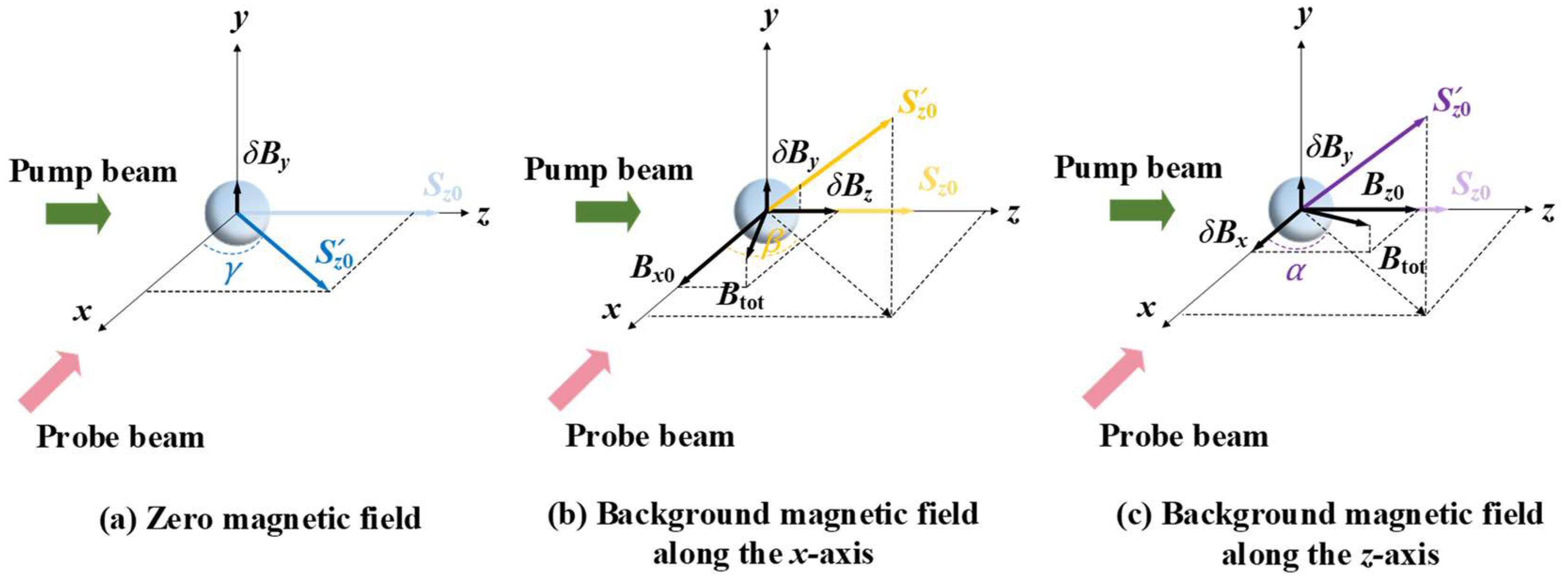
Abstract
:1. Introduction
2. Methods
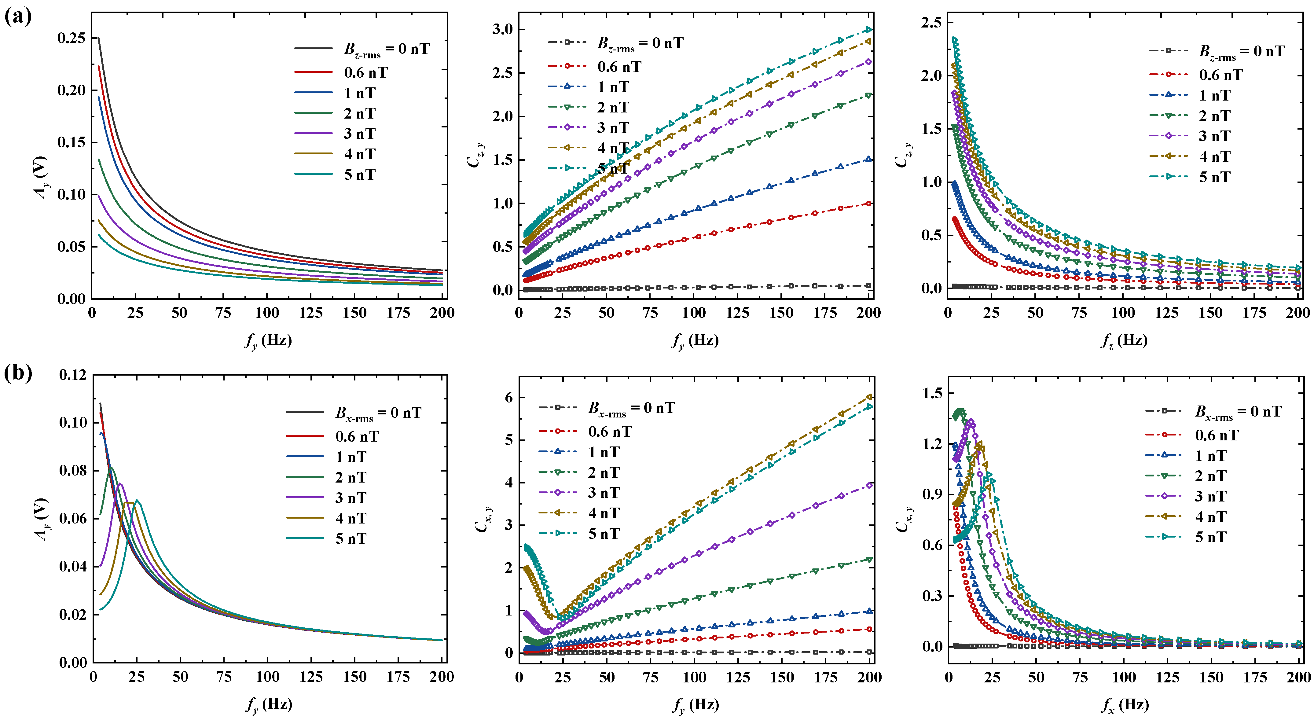
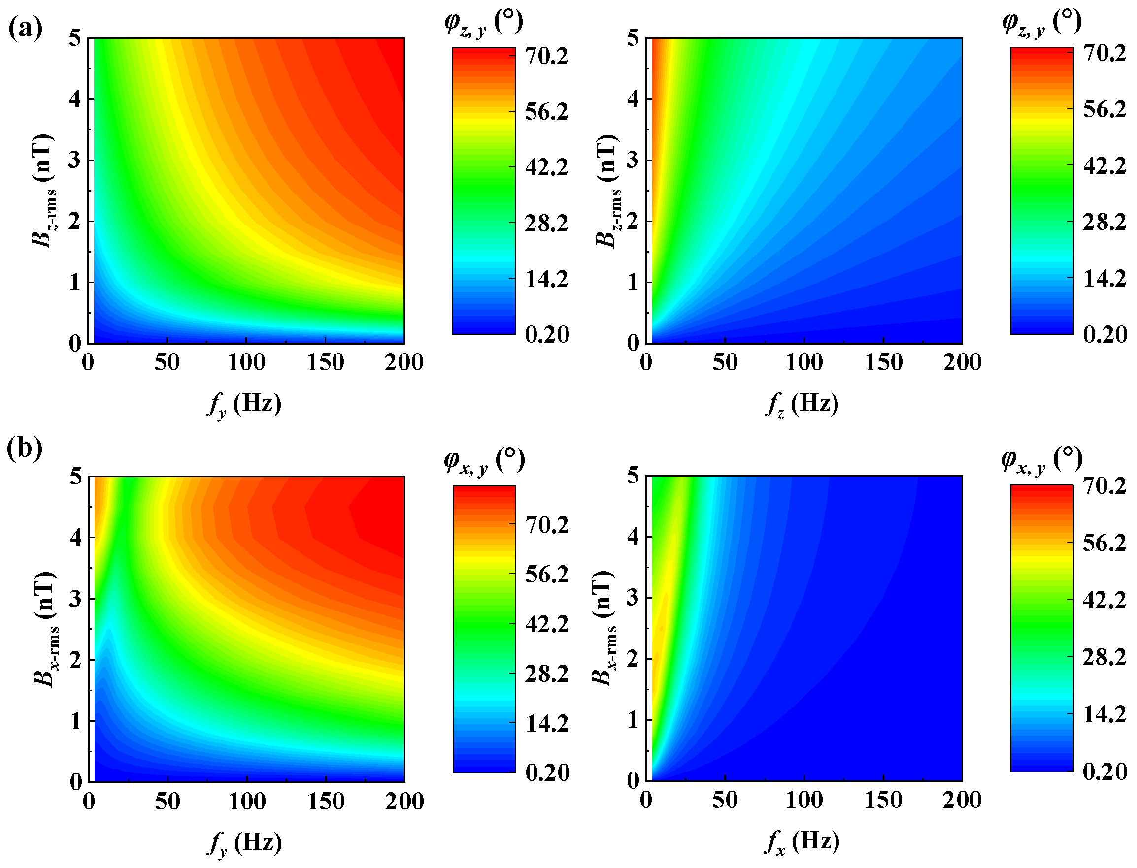
2.1. Cross-Axis Coupling Effect between z-and y-Axes under Bx0
2.2. Cross-Axis Coupling Effect between x- and y-Axes under Bz0
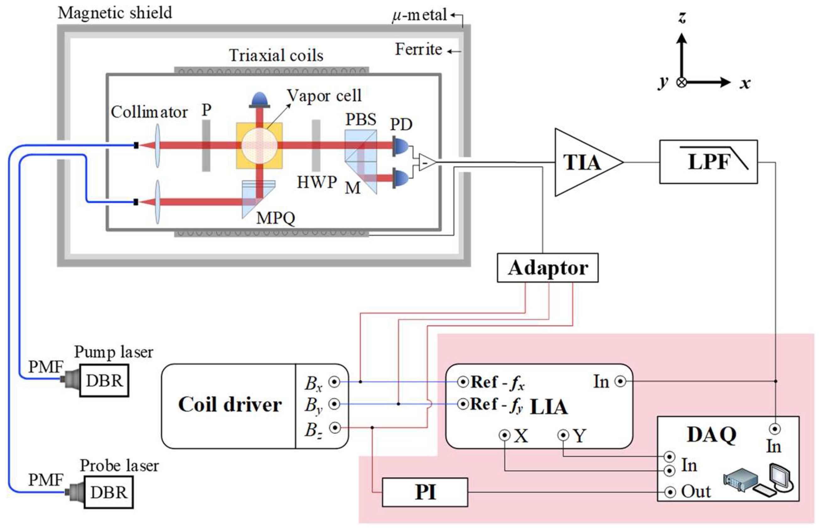
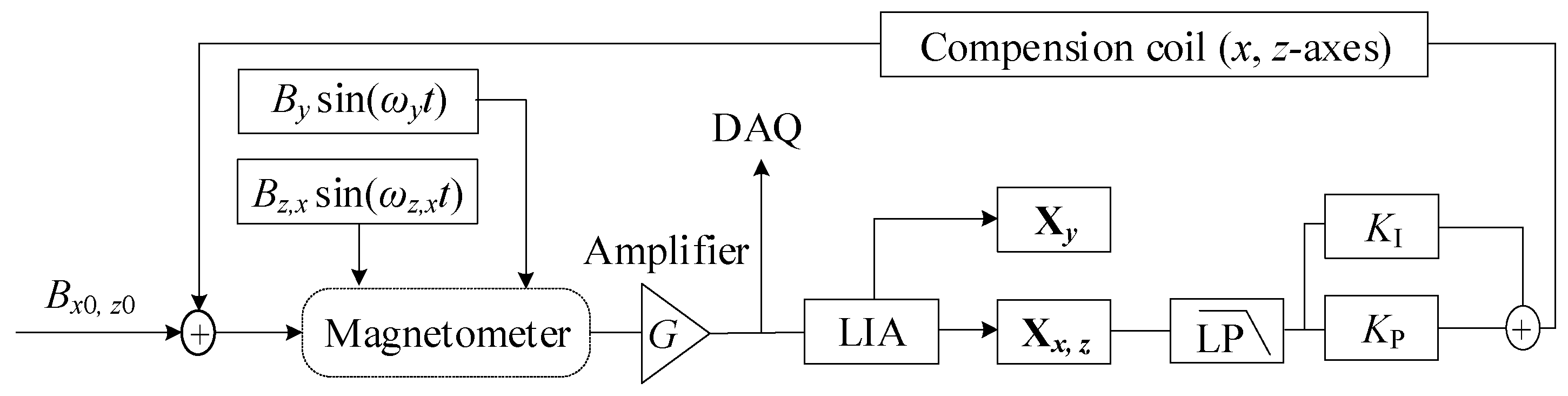
3. Experimental Setup and Procedure
4. Results and Discussion
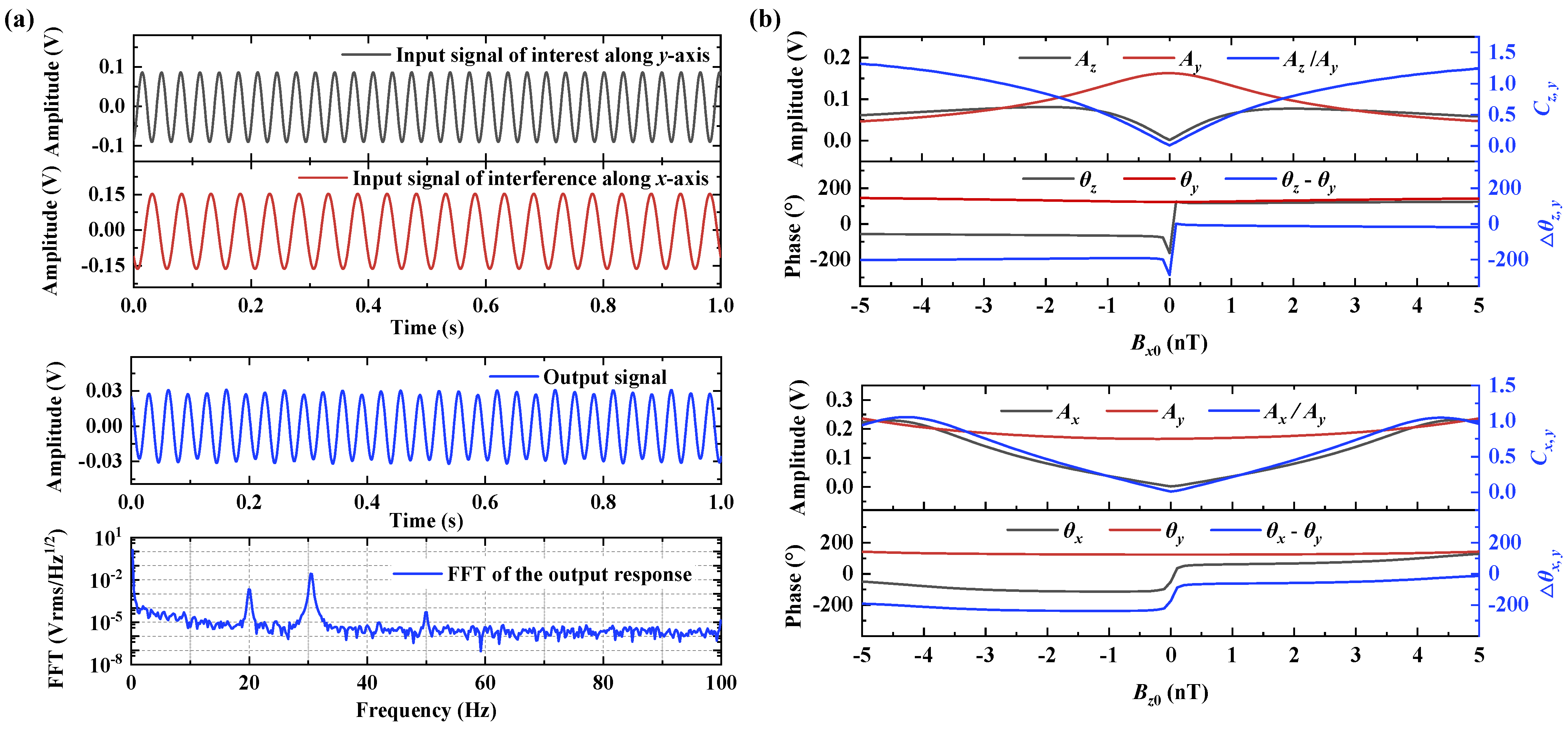
4.1. Cross-Axis Coupling Coefficient and Tilting Degree Measurement
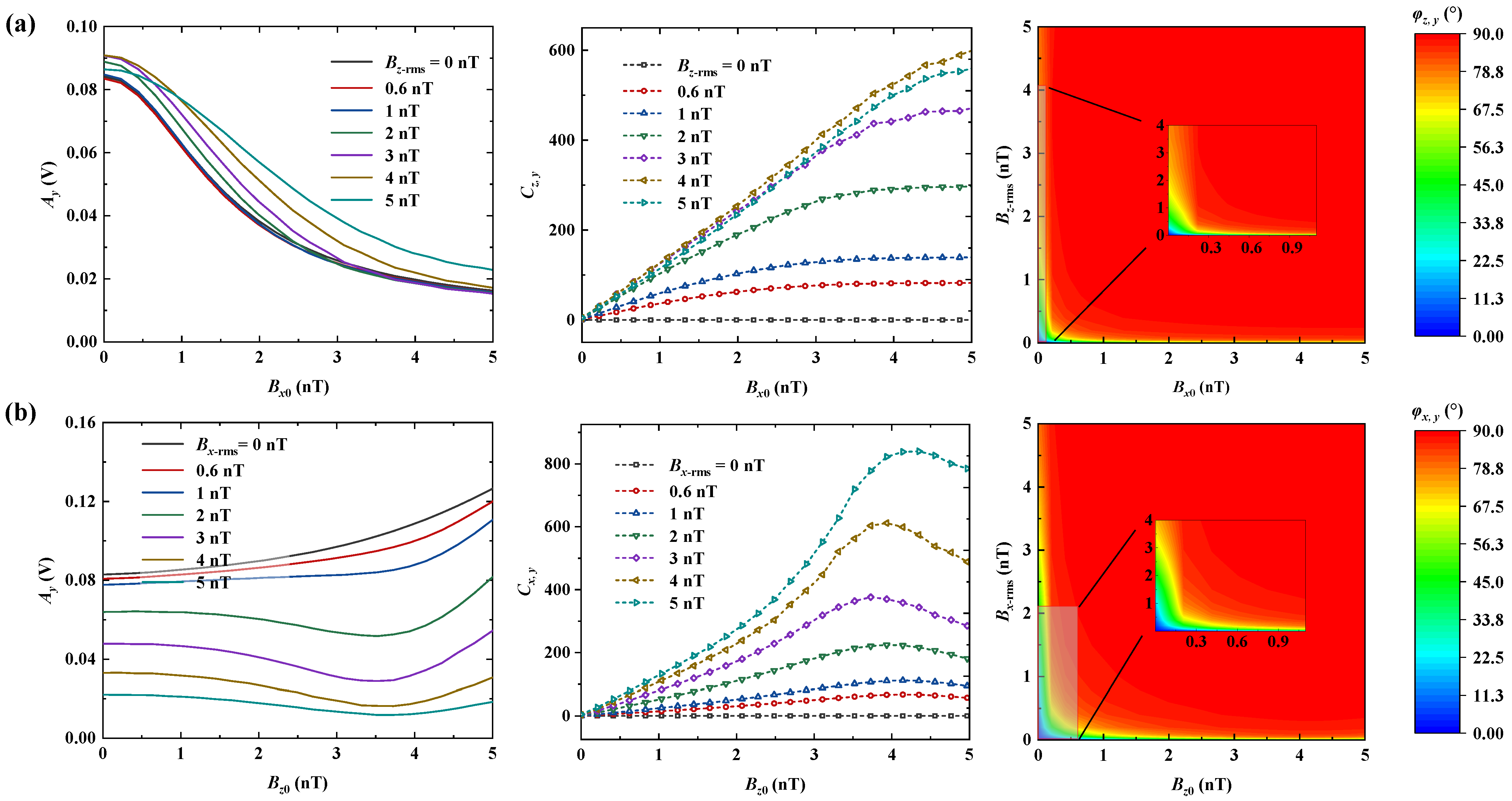
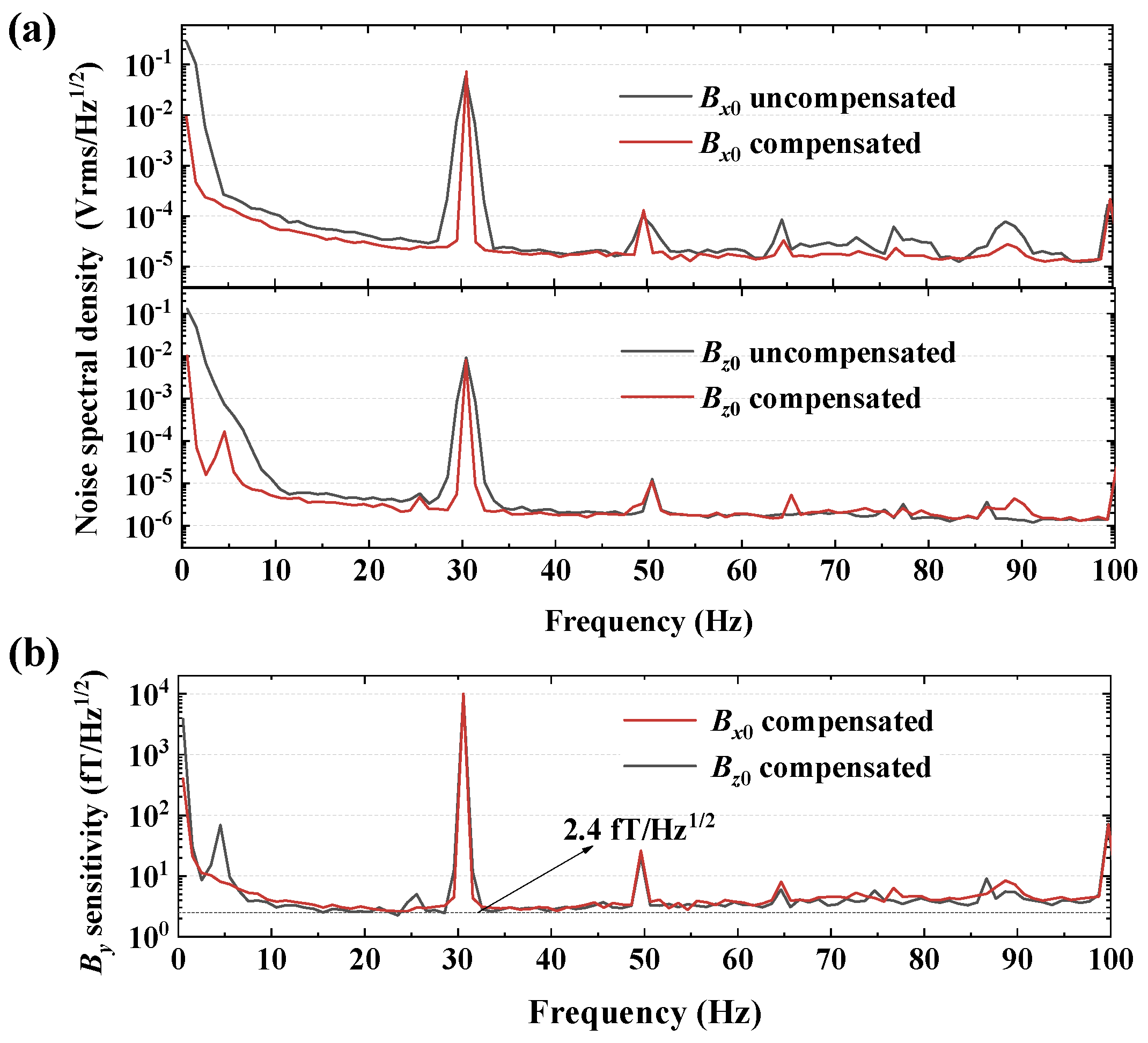
4.2. Suppression of the Cross-Axis Coupling Effect
5. Conclusions
Author Contributions
Funding
Institutional Review Board Statement
Informed Consent Statement
Data Availability Statement
Conflicts of Interest
References
- Allred, J.C.; Lyman, R.N.; Kornack, T.W.; Romalis, M.V. High-sensitivity atomic magnetometer unaffected by spin-exchange relaxation. Phys. Rev. Lett. 2002, 89, 130801. [Google Scholar] [CrossRef] [PubMed] [Green Version]
- Li, R.; Baynes, F.N.; Luiten, A.N.; Perrella, C. Continuous high-sensitivity and high-bandwidth atomic magnetometer. Phys. Rev. Appl. 2020, 14, 064067. [Google Scholar] [CrossRef]
- Kominis, I.K.; Kornack, T.W.; Allred, J.C.; Romalis, M.V. A subfemtotesla multichannel atomic magnetometer. Nature 2003, 422, 596–599. [Google Scholar] [CrossRef] [PubMed]
- Rea, M.; Holmes, N.; Hill, R.; Boto, E.; Leggett, J.; Edwards, L.J.; Woolger, D.; Dawson, E.; Shah, V.; Osborne, J.; et al. Precision magnetic field modelling and control for wearable magnetoencephalography. Neuroimage 2021, 241, 118401. [Google Scholar] [CrossRef]
- An, N.; Cao, F.; Li, W.; Wang, W.; Xu, W.; Wang, C.; Xiang, M.; Gao, Y.; Sui, B.; Liang, A.; et al. Imaging somatosensory cortex responses measured by OPM-MEG: Variational free energy-based spatial smoothing estimation approach. iScience 2022, 25, 103752. [Google Scholar] [CrossRef] [PubMed]
- Hauk, O.; Stenroos, M.; Treder, M.S. Towards an objective evaluation of EEG/MEG source estimation methods—The linear approach. Neuroimage 2022, 255, 119177. [Google Scholar] [CrossRef]
- Kornack, T.W.; Smullin, S.J.; Lee, S.K.; Romalis, M.V. A low-noise ferrite magnetic shield. Appl. Phys. Lett. 2007, 90, 223501. [Google Scholar] [CrossRef] [Green Version]
- Romalis, M.V.; Dang, H.B. Atomic magnetometers for materials characterization. Mater. Today 2011, 14, 258–262. [Google Scholar] [CrossRef]
- Colombo, S.; Lebedev, V.; Tonyushkin, A.; Pengue, S.; Weis, A. Imaging magnetic nanoparticle distributions by atomic magnetometry-based susceptometry. IEEE Trans. Med. Imag. 2020, 39, 922–933. [Google Scholar] [CrossRef]
- Li, S.; Lu, J.; Ma, D.; Wang, K.; Gao, Y.; Sun, C.; Han, B. Measurement of nonorthogonal angles of a three-axis vector optically pumped magnetometer. IEEE Trans. Instrum. Meas. 2022, 71, 7001109. [Google Scholar] [CrossRef]
- Brookes, M.J.; Boto, E.; Rea, M.; Shah, V.; Osborne, J.; Holmes, N.; Hill, R.M.; Leggett, J.; Rhodes, N.; Bowtell, R. Theoretical advantages of a triaxial optically pumped magnetometer magnetoencephalography system. Neuroimage 2021, 236, 118025. [Google Scholar] [CrossRef] [PubMed]
- Boto, E.; Holmes, N.; Leggett, J.; Roberts, G.; Shah, V.; Meyer, S.S.; Munoz, L.D.; Mullinger, K.J.; Tierney, T.M.; Bestmann, S.; et al. Moving magnetoencephalography towards real-world applications with a wearable system. Nature 2018, 555, 657–661. [Google Scholar] [CrossRef] [PubMed] [Green Version]
- Hill, R.; Boto, E.; Holmes, N.; Hartley, C.; Seedat, Z.; Leggett, J.; Roberts, G.; Shah, V.; Tierney, T.; Woolrich, M.; et al. A tool for functional brain imaging with lifespan compliance. Nat. Commun. 2019, 10, 4785. [Google Scholar] [CrossRef] [PubMed] [Green Version]
- Yan, Y.; Lu, J.; Zhou, B.; Wang, K.; Liu, Z.; Li, X.; Wang, W.; Liu, G. Analysis and correction of the crosstalk effect in a three-axis SERF atomic magnetometer. Photonics 2022, 9, 654. [Google Scholar] [CrossRef]
- Piil-Henriksen, J.; Merayo, J.M.G.; Nielsen, O.V.; Petersen, H.; Petersen, J.R.; Primdahl, F. Digital detection and feedback fluxgate magnetometer. Meas. Sci. Technol. 1996, 7, 897–903. [Google Scholar] [CrossRef]
- Zhang, R.; Ding, Y.; Yang, Y.; Zheng, Z.; Chen, J.; Peng, X.; Wu, T.; Guo, H. Active magnetic-field stabilization with atomic magnetometer. Sensors 2020, 20, 4241. [Google Scholar] [CrossRef]
- Iivanainen, J.; Zetter, R.; Grön, M.; Hakkarainen, K.; Parkkonen, L. On-scalp MEG system utilizing an actively shielded array of optically-pumped magnetometers. Neuroimage 2019, 194, 244–258. [Google Scholar] [CrossRef]
- Cohen-Tannoudji, C.; Dupont-Roc, J.; Haroche, S.; Laloë, F. Diverses résonances de croisement de niveaux sur des atomes pompés optiquement en champ nul II. Applications à la mesure de champs faibles. Rev. Phys. Appl. 1970, 5, 102–108. [Google Scholar] [CrossRef]
- Borna, A.; Iivanainen, J.; Carter, T.R.; McKay, J.; Taulu, S.; Stephen, J.; Schwindt, P.D.D. Cross-axis projection error in optically pumped magnetometers and its implication for magnetoencephalography systems. Neuroimage 2022, 247, 118818. [Google Scholar] [CrossRef]
- Jiang, M.; Xu, W.; Li, Q.; Wu, Z.; Suter, D.; Peng, X. Interference in atomic magnetometry. Adv. Quantum Technol. 2020, 3, 2000078. [Google Scholar] [CrossRef]
- Sakamoto, Y.; Bidinosti, C.P.; Ichikawa, Y.; Sato, T.; Ohtomo, Y.; Kojima, S.; Funayama, C.; Suzuki, T.; Tsuchiya, M.; Furukawa, T.; et al. Development of high-homogeneity magnetic field coil for 129Xe EDM experiment. HyInt 2015, 230, 141–146. [Google Scholar] [CrossRef]
- Ding, Z.; Huang, Z.; Pang, M.; Han, B. Iterative optimization algorithm to design bi-planar coils for dynamic magnetoencephalography. IEEE. Trans. Ind. Electron. 2022, 70, 2085–2094. [Google Scholar] [CrossRef]
- Li, Y.; Xu, J.; Kang, X.; Fan, Z.; Dong, X.; Gao, X.; Zhuang, S. Design of highly uniform three-dimensional square magnetic field coils for external magnetic shielding of magnetometers. Sens. Actuator A Phys. 2021, 331, 113037. [Google Scholar] [CrossRef]
- Lu, Y.; Yang, Y.; Zhang, M.; Wang, R.; Jiang, L.; Qin, B. Improved square-coil configurations for homogeneous magnetic field generation. IEEE Trans. Ind. Electron. 2022, 69, 6350–6360. [Google Scholar] [CrossRef]
- Yan, Y.; Lu, J.; Zhang, S.; Lu, F.; Yin, K.; Wang, K.; Zhou, B.; Liu, G. Three-axis closed-loop optically pumped magnetometer operated in the SERF regime. Opt. Express 2022, 30, 18300–18309. [Google Scholar] [CrossRef]
- Ding, Z.; Yuan, J.; Lu, G.; Li, Y.; Long, X. Three-axis atomic magnetometer employing longitudinal field modulation. IEEE Photon. J. 2017, 9, 5300209. [Google Scholar] [CrossRef]
- Jiang, L.; Liu, J.; Liang, Y.; Tian, M.; Quan, W. A single-beam dual-axis atomic spin comagnetometer for rotation sensing. Appl. Phys. Lett. 2022, 120, 074101. [Google Scholar] [CrossRef]
- Seltzer, S.J.; Romalis, M.V. Unshielded three-axis vector operation of a spin-exchange-relaxation-free atomic magnetometer. Appl. Phys. Lett. 2004, 85, 4804–4806. [Google Scholar] [CrossRef] [Green Version]
- Ledbetter, M.P.; Savukov, I.M.; Acosta, V.M.; Budker, D.; Romalis, M.V. Spin-exchange-relaxation-free magnetometry with Cs vapor. Phys. Rev. A 2008, 77, 033408. [Google Scholar] [CrossRef] [Green Version]
- Ma, D.; Lu, J.; Fang, X.; Yang, K.; Wang, K.; Zhang, N.; Han, B.; Ding, M. Parameter modeling analysis of a cylindrical ferrite magnetic shield to reduce magnetic noise. IEEE. Trans. Ind. Electron. 2022, 69, 991–998. [Google Scholar] [CrossRef]
- Ma, D.; Lu, J.; Fang, X.; Wang, K.; Wang, J.W.; Zhang, N.; Chen, H.; Ding, M.; Han, B. Analysis of coil constant of triaxial uniform coils in Mn–Zn ferrite magnetic shields. J. Phys. D 2021, 54, 275001. [Google Scholar] [CrossRef]


Publisher’s Note: MDPI stays neutral with regard to jurisdictional claims in published maps and institutional affiliations. |
© 2022 by the authors. Licensee MDPI, Basel, Switzerland. This article is an open access article distributed under the terms and conditions of the Creative Commons Attribution (CC BY) license (https://creativecommons.org/licenses/by/4.0/).
Share and Cite
Lu, F.; Wang, S.; Xu, N.; Li, B.; Lu, J.; Han, B. Analysis and Suppression of the Cross-Axis Coupling Effect for Dual-Beam SERF Atomic Magnetometer. Photonics 2022, 9, 792. https://doi.org/10.3390/photonics9110792
Lu F, Wang S, Xu N, Li B, Lu J, Han B. Analysis and Suppression of the Cross-Axis Coupling Effect for Dual-Beam SERF Atomic Magnetometer. Photonics. 2022; 9(11):792. https://doi.org/10.3390/photonics9110792
Chicago/Turabian StyleLu, Fei, Shuying Wang, Nuozhou Xu, Bo Li, Jixi Lu, and Bangcheng Han. 2022. "Analysis and Suppression of the Cross-Axis Coupling Effect for Dual-Beam SERF Atomic Magnetometer" Photonics 9, no. 11: 792. https://doi.org/10.3390/photonics9110792