Quantum Tomography of Two-Qutrit Werner States


College of Mathematics, Taiyuan University of Technology, Taiyuan 030024, China
*
Author to whom correspondence should be addressed.
Photonics 2022, 9(10), 741; https://doi.org/10.3390/photonics9100741
Submission received: 20 September 2022
/
Revised: 1 October 2022
/
Accepted: 4 October 2022
/
Published: 8 October 2022
(This article belongs to the Special Issue Photonic State Tomography: Methods and Applications)
Abstract
:In this article, we introduce a framework for two-qutrit Werner states tomography with Gaussian noise. The measurement scheme is based on the symmetric, informationally complete positive operator-valued measure. To make the framework realistic, we impose the Gaussian noise on the measured states numbers. Through numerical simulation, we successfully reconstructed the two-qutrit Werner states in various experimental scenarios and analyzed the optimal scenario from four aspects: fidelity, purity, entanglement, and coherence.
1. Introduction
Quantum state tomography (QST) plays an important role in the field of quantum information. It can determine the mathematical representation of an unknown quantum system by measuring a large number of replicated quantum states to estimate them in real time [1]. The tomography of entangled photon pairs, as a specific form of QST, has been used to characterize the quantum states of light [2]. Because noise and systematic errors exist in any quantum measurement process, statistical methods are needed to reconstruct the actual quantum states [3]. There are various methods of quantum-state estimation, but we can compare the efficiency of each method to choose the optimal estimation method.
There are many works about QST in different noise scenarios. In the work of Ref. [4], Artur Czerwinski introduced a framework for QST and the entanglement quantification of two-qubit Werner states that were encoded on photon pairs in the polarization degree of freedom. The Poisson noise was imposed on the measured photon counts. In the work of Ref. [5], the author investigated the problem of entanglement characterization by polarization measurements combined with maximum likelihood estimation (MLE). A realistic scenario was considered with measurement results distorted by three types of errors: the Poisson noise, dark counts, and random rotations. In the work of Ref. [6], the author introduced a framework for Hamiltonian tomography of multiqubit systems with random noise. The quantum quench protocol to reconstruct a many-body Hamiltonian was adopted by local measurements that were distorted by random unitary operators and time uncertainty. However, as different scenarios, other kinds of experimental noise also need to be considered. More specifically, it is also interesting that we study QST in the case of Gaussian noise, which is more complex than Poisson noise. Moreover, quntum coherence also should be studied as an important research object to evaluate the QST model because it is also a special feature of quantum mechanic such as entanglement and other quantum correlations.
The goal of our scheme is to estimate the quantum states by using the results of measurements. In the case of a positive operator-valued measure (POVM) [7], if a measurement scheme provides complete knowledge about the state of the system, we can say that is an informationally complete POVM [8]. For a given quantum system, there are various different measurement operators that can obtain the complete characterization of the quantum state. In our work, we utilize a particular case of POVM that is called a symmetic, informationally complete, positive operator-valued measure (SIC-POVM).
In the model of our article, we consider that state tomography and quantum correlations quantification can be described by two-qutrit Werner states. The SIC-POVMs are used to obtain the probability corresponding to each measurement outcomes. In order to make the model more realistic, the influence of Gaussian noise on the measurement process is imposed. Then, the density matrices of the estimated unknown states are obtained by a modified -estimator [9]. We perform numerical simulation experiments on noise scenarios of different intensities and graphically illustrate the accuracy of our model under these scenarios.
2. Materials and Methods
2.1. Two-Qutrit Werner State
In 1989, R. Werner introduced the non-classical correlation mixed quantum states [10]. Among these, the two-qubit Werner state can be expressed as follows:
where U is a unitary operator. Additionally, the meaning of Formula (1) is the density matrices of Werner states remain unchanged after the transformation in Formula (1). Furthermore, Werner states can be expressed as
where and are two real paramters; I denotes the identity operator; and T is a flip operator, which acts as .
Suppose denotes the standard basis in d-dimensional Hilbert space, then T takes the form:
Due to , the two-qutrit Werner states can be expressed as
where is the identity matrix of 9 × 9; the quantum state is the Bell state composed of subsystems A and B (with the largest degree of entanglement); and is the distribution coefficient, which determines the proportion of and in the Werner state.
Werner states play an important role in quantum information theory, for instance, entanglement purification [11]. They have also been used for a description of noisy quantum channels [12]. The properties of Werner states in arbitrary dimensions, for example, concurrence-based entanglement measures [13], remain relevant topics. Therefore, it appears justified to investigate the quantum tomography of two-qutrit Werner states with noisy measurements.
2.2. Measurements
Let us assume there is a set of normalized vectors that belong to d-dimensional Hilbert space such that
Then, the set of rank-one projectors defined as
constitutes a symmetric, informationally complete, positive operator-valued measure (SIC-POVM).
The measurement scheme implemented in our work is based on the SIC-POVM in three-dimensional Hilbert space. When , the SIC-POVM can be described by the following nine vectors:
where denotes the standard basis in Hilbert space. Then, our measurement operators can be defined: , , which satisfy . These nine measurement operators are sufficient to perform single-qubit tomography [14]. Additionally, these measurements are minimal, but they allow for efficient and reliable single-qubit tomography. SIC-POVMs, which belong to the class of minimal informationally complete quantum measuremenmts, are in many ways optimal since the ideal measurements in quantum physics are not orthogonal bases [15]. Therefore, for two-qutrit Werner states characterized by Formula (4), we can utilize , to represent the measurement operators.
2.3. Quantum-State Estimation with Gaussian Noise
Suppose a quantum system is in one of a number of states , where i is an index, with respective probabilities . The density operator for the system is defined by the following equation:
For the state , the probability of obtaining measurement outcome k is . Then, the probability of obtaining measurement outcome k is
Hence, for the Werner states , the probability of obtaining measurement outcome k is
Suppose the number of quantum states we use for each measurement is N; then, the number of quantum states with the measurement outcome k is
To make our model more realistic, we impose Gaussian noise. Under the influence of Gaussian noise, N becomes , which obeys the normal distribution: , that is to say, the number of quantum states for each measurement is selected randomly from the Gaussian distribution characterized by the mean value and standard deviation . Let , thus, after imposing Gaussian noise, the number of quantum states with the measurement result of k can be modeled numerically as
Because is a random variable subject to normal distribution, it still follows the normal distribution after multiplication by a non-zero constant , but the expectation and variance will change, that is, the expectation will become , and the variance will become . Hence, obeys the following normal distribution:
However, when performing QST, we assume that we know nothing about the states. For this reason, the expected number of unknown states with measurement result k is
where represents a general 9 × 9 density matrix. According to Cholesky’s decomposition [2,16], the unknown quantum state we need to estimate can be expressed as follows:
where
and j is the imaginary unit; then, we only need to estimate , which are 81 real parameters.
For any that satisfies , the process of quantum-state estimation is reduced to determining the 81 parameters that characterize R. To find the 81 parameters that optimally fit the noisy measurements, we use a modified -estimator, see, Ref. [9]. Thus, we search for the minimum value of the following function:
This procedure allows one to simulate an experimental scenario for any input state . First, we generate the noisy quantum states numbers Formula (12), and then we can recover the state by finding the parameters , for which the function reaches its minimum.
3. Numerical Results and Analysis
When the numerical simulation of our model is conducted, the interval of [0,1] is divided into 20 equal parts, and each one is put into Formula (17) to find the corresponding ; consequently, the corresponding are computed. In different noise scenarios, the N and are changed, i.e., and . Additionally, these scenarios are compared in the form of images from the perspectives of fidelity, purity, entanglement, and coherence. Quantum fidelity is computed to quantify the accuracy of states reconstruction. Quantum purity is computed to analyze how much the states are mixed. The concurrence and norm of coherence are used to evaluate how well quantum features are preserved for the reconstructed states.
3.1. Fidelity
First, every input Werner state is compared with the estimated quantum state , by computing the quantum fidelity:
It is commonly used to assess the accuracy of QST frameworks, in particular, under imperfect measurement settings, see Ref. [17]. Obviously, when the estimated quantum states are equal to the input Werner states , the theoretical value of is 1. When the estimated quantum states are not equal input Werner states , the higher the fidelity, the better the experimental results.
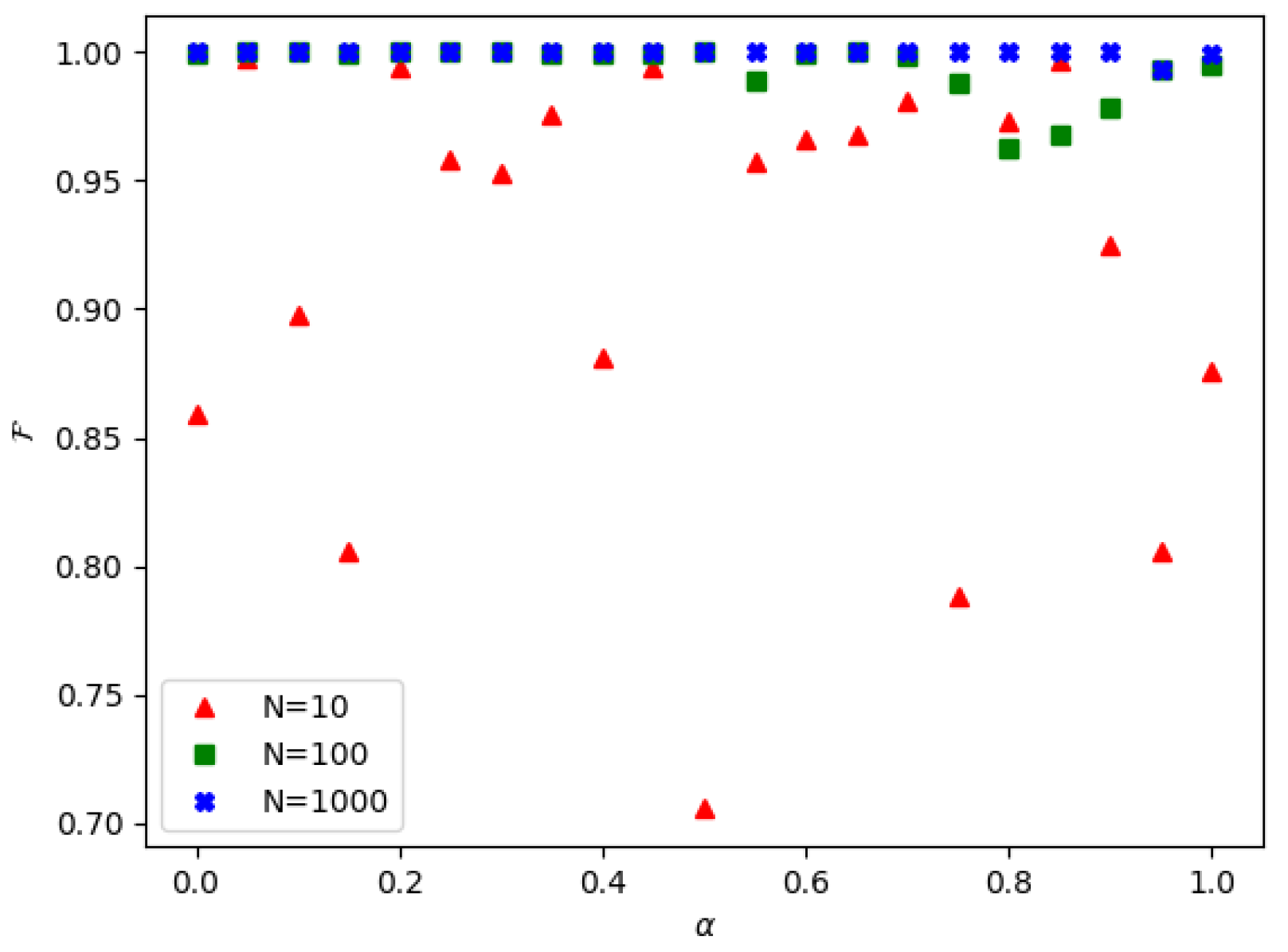
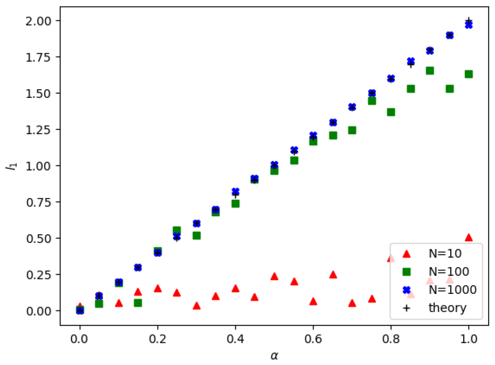
In Figure 1, is 1 and N is variable in the current situation. The blue, green, and red dots represent the fidelity when , respectively. It can be clearly seen that the fidelity is almost close to the theoretical value 1 when N is 1000. When N is equal to 100, the approximate degree between the estimated values and the theoretical value 1 is obviously not as close as the condition when N is equal to 1000. When N is equal to 10, the estimated values and the theoretical value 1 have a large deviation, only a few points are close to the theoretical value 1. In addition, in the current situation (), when gradually increases, generally shows a decreasing trend, which means that the fidelity of the reconstructed states is lower when input Werner states are closer to the pure states.
In Figure 2, N is equal to 1000 and is variable in the current situation. The blue, green, and red dots represent the fidelity when , respectively. It can be clearly seen that when , the fidelity is close to the theoretical value 1, but as increases, our experimental fidelity starts to drop significantly. This shows that our experimental fidelity gradually tends to deviate from the theoretical value 1 as the increases.
Since fidelity is the most important factor in evaluating the efficiency of our model, we need to display our experimental results in a more intuitive histogram. As shown in the Figure 3, we have taken five special values of , and we can more intuitively see that when is fixed at 1, the larger N is, the higher the fidelity of the experimentally reconstructed quantum state is. Similarly, as shown in the Figure 4, when N is fixed to 1000, the smaller is, the higher the fidelity of the quantum state reconstructed by the experiment is. When N = 1000, , the fidelity of the reconstructed states reaches above 0.99, which is an excellent result.
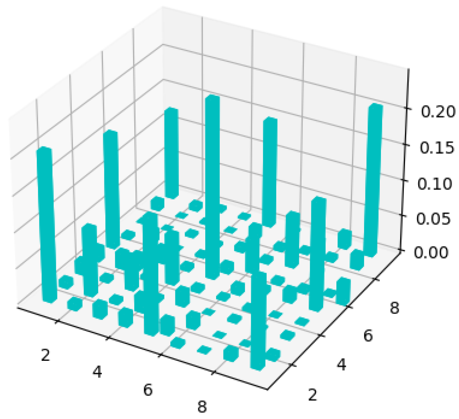
In general, when N is larger and is smaller, the efficiency of our model is better. In the Figure 5 and Figure 6, when N = 1000, = 1, we show the density matrix tomography of the experimentally reconstructed two-qutrit Werner states of = 0.5 and 1.
The tomography of the two-qubit Werner states can also be applied to our model; of course, we need to replace the SIC-POVM in the three-dimensional Hilbert space with the SIC-POVM in the two-dimensional Hilbert space. For example, when , the SIC-POVM can be described by the following four vectors:
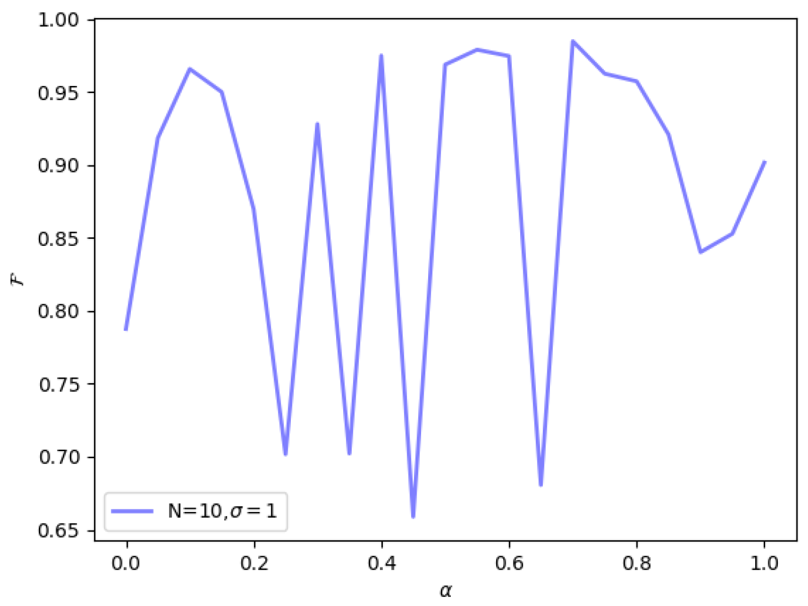
As shown in the Figure 7, after we perform the same experimental process on the two-qubit Werner states , in terms of fidelity, when N = 1000 and 100 (), similar results can be obtained for the two-qutrit Werner states. However, when N = 10 (), as shown in the Figure 8, we find that the fidelity of the two-qubit Werner states does not obviously decrease with the increase in but fluctuates irregularly.
3.2. Purity
Let us analyze the purity of the experimental results of two-qutrit Werner states. Quantum purity is computed to analyze how much the states are mixed. We utilize the trace of the density matrix’s square to express purity. Hence, we use to calculate the theoretical purity and use to calculate the estimated states’ purity [7].
In Figure 9, is 1 and N is variable in the current situation. The black dots represent the theoretical purity values, and the blue, green, and red dots represent the purity values of the quantum states estimated when , respectively. It can be seen that when , the estimated values are almost close to the theoretical values. When , the closeness of the estimated values to the theoretical values is obviously worse than when . When , the estimated values obviously deviate from the theoretical values. It is worth noting that at , whether N = 1000, 100, or 10, the estimated values of purity are the same; when increases from 0.4 to 1, the gap between these three scenarios gradually increase.
In Figure 10, N is 1000 and is variable in the current situation. The black dots represent the theoretical purity values, and the blue, green, and red dots represent the purity when , respectively. We can clearly see that when , the estimated values are almost close to the theoretical values. However, as increases, our experimental accuracy of purity tends to drop significantly. This shows that our experimental values gradually tend to deviate from the theoretical values as the increases.
In a word, when N is larger and is smaller, the closer the experimental results of purity are to the theoretical value.
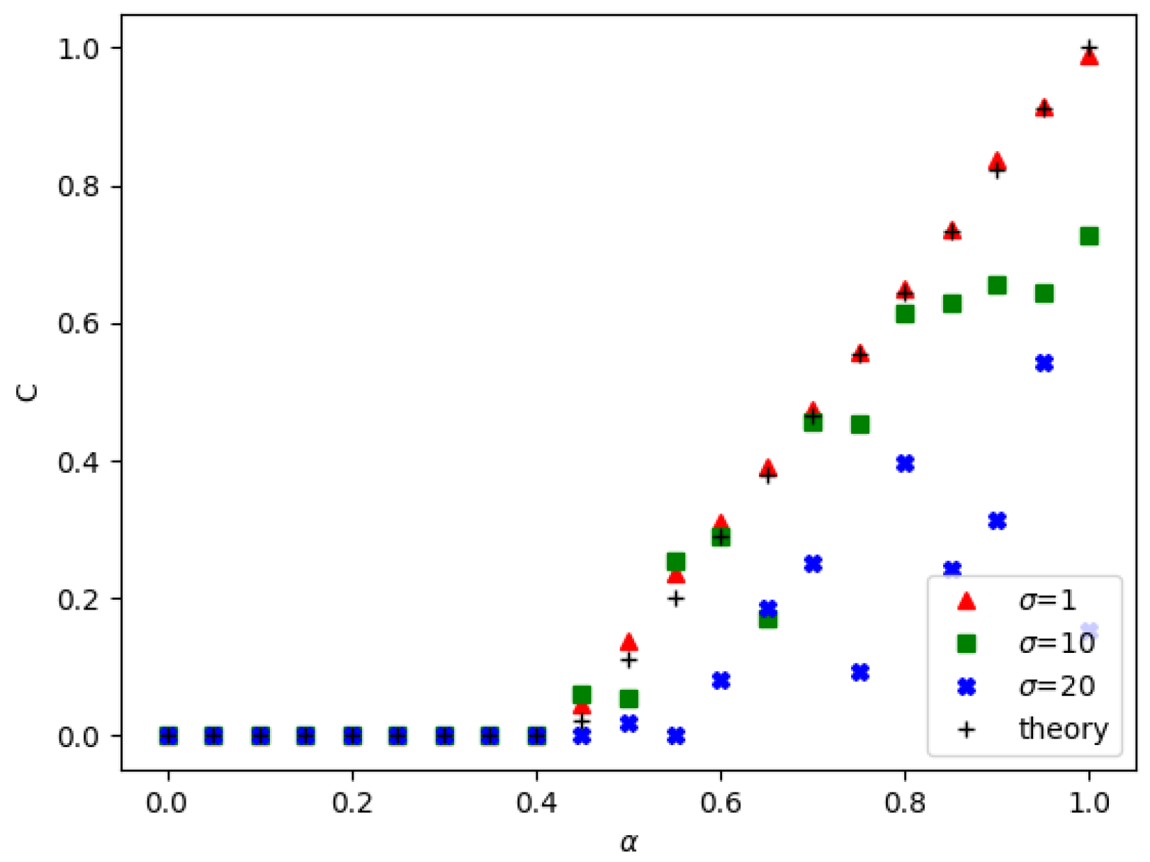
3.3. Entanglement
For two-qutrit Werner states , we compute the concurrence, , which quantifies the amount of entanglement in the system described by the density matrix [18,19]. Then, the entanglement quantification of two-qutrit Werner states can be represented as follows:
where is the eigenvalue’s modulo of the density matrix , and .
For any density matrix , the concurrence satisfies 01. We have = 1 for maximally entangled states and = 0 for separate states. Thus, the concurrence can be considered an entanglement monotone, which means it can be applied to quantify quantum entanglement, see Refs. [20,21,22,23]. Concurrence is directly connected to another fundamental measure, which is called the entanglement of formation [24,25].
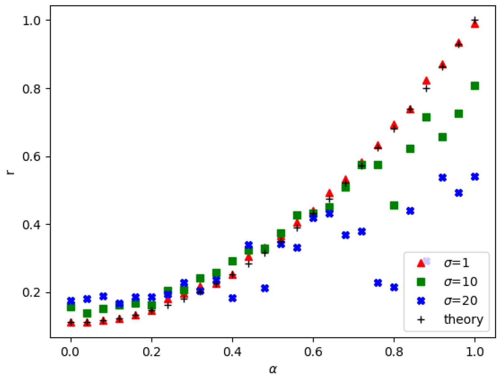
In Figure 11, is 1 and N is variable in the current situation. The black dots represent the theoretical values of the concurrence, and the blue, green, and red dots represent the concurrence of the quantum states estimated when , respectively. It can be seen that when , the estimated values are very close to the theoretical values. When N is 100, it also can be seen that the deviation between the estimated values and the theoretical values is greater than when N is 1000. When N is reduced to 10, the estimated values almost completely deviate from the theoretical values.
In Figure 12, and is variable in the current situation. The black dots represent the theoretical concurrence values, and the blue, green, and red dots represent the concurrence when , respectively. It can be clearly seen that when = 1, the experimental concurrence values are almost close to the theoretical values. However, as increases, the experimental accuracy of concurrence starts to drop significantly. This shows that the experimental values gradually tend to deviate from the theoretical values as the increases.
3.4. Coherence
Under a fixed reference basis, the norm of coherence of state is defined by
hence, we can obtain
and it can be easily found that the norm coherence of is monotonic and proportional to the parameter .
Although many coherence measures have been proposed, the norm of coherence stands out as one of the most important measures that is easily computable [26]. It is useful in studying speedup in quantum computation, such as in the Deutsch–Jozsa algorithm [27] and the Grover algorithm [28]. It features prominently in alternative formulations of uncertainty relations, complementarity relations [29], and wave-particle duality in multipath interferometers [30]. It plays a crucial role in quantifying the cohering and decohering powers of quantum operations [31]. In addition, the norm of coherence sets an upper bound for another important coherence measure, the robustness of coherence [32].
In Figure 13, is 1 and N is variable in the current situation. The black dots represent the theoretical values of the norm, and the blue, green, and red dots represent the norm of the quantum state estimated when , respectively. It can be seen that when , the estimated values are very close to the theoretical values. When N is 100, it also can be found that the deviation between the estimated values and the theoretical values is greater than when . When N is reduced to 10, the estimated values almost completely deviate from the theoretical values.
In Figure 14, N is 1000 and is variable in the current situation. The black dots represent the theoretical norm values, and the blue, green, and red dots represent the norm the norm of coherence when , respectively. It can be clearly seen that when , the experimental norm of the coherence values is almost close to the theoretical values. However, as increases, the experimental accuracy of the norm starts to drop significantly. This shows that the experimental values gradually begin to deviate from the theoretical values as the increases.
4. Discussion
In this article, we introduce a method for estimating two-qutrit Werner states under Gaussian noise based on SIC-POVMs. The efficiency of our framework or our model’s resistance to Gaussian noise is shown by how much the experimental values deviate from the theoretical values. It is investigated in the scenarios of , , and , . Additionally, these scenarios were compared in the form of images from the perspectives of fidelity, purity, entanglement, and coherence.
We conclude that when and , our model can resist Gaussian noise well, but when N decreases to 100, the robustness of our model starts to drop. When N decreases to 10, our model’s resistance to Gaussian noise is almost lost. We also conclude that when and , our model can resist Gaussian noise very well, but when increases to 10, the robustness of our model starts to drop. When increases to 20, our model’s resistance to Gaussian noise is almost lost. Therefore, we can speculate that when both the N is larger and is smaller, our model is more resistant to Gaussian noise.
However, it is worth noting that when N = 10 and = 1, if we increase to be close to 1, the experimental values will deviate from the theoretical values to a certain extent, which means that when the Werner states are pure or close to pure, the fidelity of our model will be greatly compromised even if the number of input quantum states is not large enough. For the other three perspectives such as purity, entanglement, and coherence, our model leads to similar conclusions. This shows that Gaussian noise has a relatively large influence on the reconstruction of the pure state in our model if N is not large enough or is not small enough. However, in the case of Poisson noise, regardless of the value of N, as tends to 1, the estimated values converge to the theoretical values, see Ref. [4]. This is the major difference between Gaussian noise and Poisson noise under the QST model.
We also found that if the dimension of Werner states is increased from two-dimensional to three-dimensional, the calculation time of our algorithm will increase significantly, which will cause great trouble to the tomography of higher dimensional quantum states in the future. To solve this problem, we can limit the Gaussian random variable , such as limiting , because the probability of a Gaussian random variable falling in this interval is 0.997. In addition, when solving the minimum point of Formula (17), we used the minimize function in Python. We believe that there will be other algorithms to replace it more effectively, and we will be committed to solving this problem in future work.
5. Conclusions
This paper provides a method for two-qutrit Werner states tomography under Gaussian noise. From the perspectives of fidelity, purity, entanglement, and coherence, we conclude that when and , our model can resist Gaussian noise well. In future studies, we will investigate more precisely how the values of and N affect the experimental precision. In addition, we will study other quantum states under this model.
Author Contributions
Conceptualization, H.W. and K.H.; formal analysis, H.W.; investigation, H.W.; methodology, H.W.; project administration, K.H.; supervision, K.H.; validation, K.H.; writing—original draft, H.W.; and writing—review and editing, H.W. and K.H. All authors have read and agreed to the published version of the manuscript.
Funding
This work was supported by the National Natural Science Foundation of China (grants No. 12271394) and the Key Research and Development Program of Shanxi Province (grants No. 202102010101004).
Institutional Review Board Statement
Not applicable.
Informed Consent Statement
Not applicable.
Data Availability Statement
The data and code underlying the results presented in this paper can be obtained from the corresponding author upon reasonable request.
Conflicts of Interest
The authors declare no conflict of interest.
References
- Paris, M.G.A.; Řeháček, J. (Eds.) Quantum-State Estimation (Lecture Notes in Physics); Springer: Berlin/Heidelberg, Germany, 2004. [Google Scholar]
- D’Ariano, G.M.; Paris, M.G.A.; Sacchi, M.F. Quantum Tomography. Adv. Imaging Electron Phys. 2003, 128, 205–308. [Google Scholar]
- Hradil, Z. Quantum-state estimation. Phys. Rev. A 1997, 55R, 1561. [Google Scholar] [CrossRef] [Green Version]
- Czerwinski, A. Quantifying entanglement of two-qubit Werner states. Commun. Theor. Phys. 2021, 73, 085101. [Google Scholar] [CrossRef]
- Czerwinski, A. Entanglement Characterization by Single-Photon Counting with Random Noise. Quantum Inf. Comput 2021, 22, 1–16. [Google Scholar] [CrossRef]
- Czerwinski, A. Hamiltonian tomography by the quantum quench protocol with random noise. Phys. Rev. A 2021, 104, 052431. [Google Scholar] [CrossRef]
- Nielsen, M.A.; Chuang, I.L. Quantum Computation and Quantum Information; Cambridge University Press: London, UK, 2000. [Google Scholar]
- Busch, P. Informationally complete sets of physical quantities. Int. J. Theor. Phys. 1991, 30, 1217–1227. [Google Scholar] [CrossRef]
- Jack, B.; Leach, J.; Ritsch, H.; Barnett, S.M.; Padgett, M.J.; Franke-Arnold, S. Precise quantum tomography of photon pairs with entangled orbital angular momentum. New J. Phys. 2009, 11, 103024. [Google Scholar] [CrossRef]
- Werner, R.F. Quantum states with Einstein-Podolsky-Rosen correlations admitting a hidden-variable model. Phys. Rev. A 1989, 40, 4277–4281. [Google Scholar] [CrossRef]
- Bennett, C.H.; Brassard, G.; Popescu, S.; Schumacher, B.; Smolin, J.A.; Wootters, W.K. Purification of Noisy Entanglement and Faithful Teleportation via Noisy Channels. Phys. Rev. Lett. 1996, 76, 722. [Google Scholar] [CrossRef] [Green Version]
- Checinska, A.; Wodkiewicz, K. Separability of entangled qutrits in noisy channels. Phys. Rev. A 2007, 76, 052306. [Google Scholar] [CrossRef] [Green Version]
- Chen, K.; Albeverio, S.; Fei, S.-M. Concurrence-Based Entanglement Measure For Werner States. Rep. Math. Phys. 2006, 58, 325–334. [Google Scholar] [CrossRef]
- Řeháček, J.; Englert, B.G.; Kaszlikowski, D. Minimal qubit tomography. Phys. Rev. A 2004, 70, 052321. [Google Scholar]
- DeBrota, J.B.; Fuchs, C.A.; Stacy, B.C. The varieties of minimal tomographically complete measurements. Int.J.Quantum Inf. 2021, 19, 2040005. [Google Scholar] [CrossRef]
- James, D.F.V.; Kwiat, P.G.; Munro, W.J.; White, A.G. Measurement of qubits. Phys. Rev. A 2001, 64, 052312. [Google Scholar] [CrossRef] [Green Version]
- Yuan, H.; Zhou, Z.-W.; Guo, G.-C. Quantum state tomography via mutually unbiased measurements in driven cavity QED systems. New J. Phys. 2016, 18, 043013. [Google Scholar] [CrossRef]
- Hill, S.; Wootters, W.K. Entanglement of a Pair of Quantum Bits. Phys. Rev. Lett. 1997, 78, 5022–5025. [Google Scholar] [CrossRef] [Green Version]
- Wootters, W.K. Entanglement of Formation of an Arbitrary State of Two Qubits. Phys. Rev. Lett. 1998, 80, 2245–2248. [Google Scholar] [CrossRef] [Green Version]
- Walborn, S.P.; Souto Ribeiro, P.H.; Davidovich, L.; Mintert, F.; Buchleitner, A. Experimental determination of entanglement with a single measurement. Nature 2006, 440, 1022–1024. [Google Scholar] [CrossRef]
- Buchleitner, A.; Carvalho, A.R.R.; Mintert, F. Entanglement in Open Quantum Systems. Acta Phys. Pol. A 2007, 112, 575–588. [Google Scholar] [CrossRef]
- Neves, L.; Lima, G.; Fonseca, E.J.S.; Davidovich, L.; Padua, S. Characterizing entanglement in qubits created with spatially correlated twin photons. Phys. Rev. A 2007, 76, 032314. [Google Scholar] [CrossRef] [Green Version]
- Bergschneider, A.; Klinkhamer, V.M.; Becher, J.H.; Klemt, R.; Palm, L.; Zurn, G.; Jochim, S.; Preiss, P.M. Experimental characterization of two-particle entanglement through position and momentum correlations. Nat. Phys. 2019, 15, 640–644. [Google Scholar] [CrossRef]
- Bennett, C.H.; DiVincenzo, D.P.; Smolin, J.A.; Wootters, W.K. Mixed-state entanglement and quantum error correction. Phys. Rev. A 1996, 54, 3824–3851. [Google Scholar] [CrossRef] [PubMed]
- Horodecki, M. Entanglement measures. Quantum Inf. Comput. 2001, 1, 3–26. [Google Scholar] [CrossRef]
- Baumgratz, T.; Cramer, M.; Plenio, M.B. Quantifying Coherence. Phys. Rev. Lett. 2014, 113, 140401. [Google Scholar] [CrossRef] [PubMed] [Green Version]
- Hillery, M. Coherence as a resource in decision problems: The Deutsch-Jozsa algorithm and a variation. Phys. Rev. A 2016, 93, 012111. [Google Scholar] [CrossRef] [Green Version]
- Shi, H.-L.; Liu, S.-Y.; Wang, X.-H.; Yang, W.-L.; Yang, Z.-Y.; Fan, H. Coherence depletion in the Grover quantum search algorithm. Phys. Rev. A 2017, 95, 032307. [Google Scholar] [CrossRef] [Green Version]
- Cheng, S.; Hall, M.J.W. Complementarity relations for quantum coherence. Phys. Rev. A 2015, 92, 042101. [Google Scholar] [CrossRef] [Green Version]
- Bera, M.N.; Qureshi, T.; Siddiqui, M.A.; Pati, A.K. Duality of quantum coherence and path distinguishability. Phys. Rev. A 2015, 92, 012118. [Google Scholar] [CrossRef] [Green Version]
- Bu, K.; Kumar, A.; Zhang, L.; Wu, J. Cohering power of quantum operations. Phys. Lett. A 2017, 381, 1670. [Google Scholar] [CrossRef] [Green Version]
- Piani, M.; Cianciaruso, M.; Bromley, T.R.; Napoli, C.; Johnston, N.; Adesso, G. Robustness of asymmetry and coherence of quantum states. Phys. Rev. A 2016, 93, 042107. [Google Scholar] [CrossRef]
Figure 1.
Comparison of fidelity when .

Figure 2.
Comparison of fidelity when .

Figure 3.
Comparison of fidelity when = 1, is divided into quarters in the interval 0 to 1.

Figure 4.
Comparison of fidelity when , is divided into quarters in the interval 0 to 1.

Figure 5.
Density matrix when .

Figure 6.
Density matrix when .

Figure 7.
Fidelity of two-qubit Werner states.

Figure 8.
, fidelity of 2-qubit Wermer states.

Figure 9.
Comparison of purity when .

Figure 10.
Comparison of purity when .

Figure 11.
Comparison of concurrence: .

Figure 12.
Comparison of concurrence: .

Figure 13.
Comparison of coherence: .

Figure 14.
Comparison of coherence: .

Publisher’s Note: MDPI stays neutral with regard to jurisdictional claims in published maps and institutional affiliations. |
© 2022 by the authors. Licensee MDPI, Basel, Switzerland. This article is an open access article distributed under the terms and conditions of the Creative Commons Attribution (CC BY) license (https://creativecommons.org/licenses/by/4.0/).
Share and Cite
MDPI and ACS Style
Wang, H.; He, K. Quantum Tomography of Two-Qutrit Werner States. Photonics 2022, 9, 741. https://doi.org/10.3390/photonics9100741
AMA Style
Wang H, He K. Quantum Tomography of Two-Qutrit Werner States. Photonics. 2022; 9(10):741. https://doi.org/10.3390/photonics9100741
Chicago/Turabian StyleWang, Haigang, and Kan He. 2022. "Quantum Tomography of Two-Qutrit Werner States" Photonics 9, no. 10: 741. https://doi.org/10.3390/photonics9100741
Note that from the first issue of 2016, this journal uses article numbers instead of page numbers. See further details here.