Article

Detection Optimization of an Optically Trapped Microparticle in Vacuum with Kalman Filter

1
State Key Laboratory of Modern Optical Instrumentation, College of Optical Science and Engineering, Zhejiang University, Hangzhou 310027, China
2
Research Center for Quantum Sensing, Zhejiang Lab, Hangzhou 311121, China
*
Author to whom correspondence should be addressed.
Photonics 2022, 9(10), 700; https://doi.org/10.3390/photonics9100700
Submission received: 31 August 2022 / Revised: 20 September 2022 / Accepted: 23 September 2022 / Published: 27 September 2022
(This article belongs to the Special Issue Light Control and Particle Manipulation)

Abstract

:
The optical trapping of micro-nano particles in a high vacuum has become a popular research platform in various frontier fields of physics because of its excellent isolation from the environment. The precise measurement of particle motion information is required to analyze and control particle motion modes in traps. However, the detection accuracy is limited by measurement noise and coupling signals from other axes in microparticle optical traps. In this study, we use the Kalman filter to extract the real motion information of each axis under simulation conditions, and the results show that the Kalman filter performs well in noise suppression, improving the RMSE from 12.64 to 5.18 nm and enhancing the feedback cooling performance by approximately 27% through reducing the axes’ signal coupling ratio. We believe that as a solution to these challenges, the Kalman filter will bring a significant achievement to micrometer particle optical traps in vacuums.

1. Introduction

Since Ashkin et al., used a single-beam optical trap to levitate a 20 μ m silica sphere in 1971 [1], optical trapping has inspired various researches and applications in quantum physics, life science, and engineering. Trapping is developing rapidly towards smaller scales, including nanostructured trapping [2,3,4], on-chip optical levitation with a metalens in a vacuum [5], multiplexed near-field optical trapping [6], light polarization measurements [7], single-cell manipulation [8], on-chip protein sensing [9], and many other areas. Tongcang Li et al. used an optical trap in a vacuum to measure the instantaneous velocity of a Brownian particle [10] and to cool an optically trapped microsphere from room temperature to millikelvins [11], demonstrating the great potential of optical traps in frontier physics. Optical trapping in vacuums has also been applied to precise force and acceleration measurements and reached sub-100 ng/ Hz and sub-aN/ Hz spectral sensitivity while providing a much larger dynamic range than clamped resonators because of its outstanding decoupling from environment noise vibrations and gas molecule collisions [12,13,14,15,16,17]. Optical trapping, which is enabled by the ability to detect ultra-weak forces and acceleration, is expected to make a significant contribution to fields, such as searching for non-Newtonian interactions at the micrometer scale [18,19], high-frequency gravitational waves [20], and dark matter [21].
To achieve high acceleration sensitivity, the micrometer particle is more suitable than the nanometer particle because of the inverse relationship between the minimum measurable acceleration and the square of the particle radius [13]. Before the measurement process, the particle must maintain stable suspension in an ultra-high vacuum with the help of a feedback control system to suppress the Brownian motions of the trapped particle. The rapid and accurate displacement detection via photodiodes is the key part of the feedback control system. However, due to the close resonance peaks and detection coupling in microparticle optical traps [11,22], extracting the real signal requires not only considering the measurement noise that appears in nanoparticle optical traps but also the coupling signal from other axes. This coupling situation appears more frequently in horizontal counter-propagating dual-beam optical traps, which provide a larger response bandwidth compared to the common single vertically upward optical traps. Zhu et al. added three variable irises into the detection optics and achieved a coupling detection ratio reduction of 49.1 dB and 22.9 dB in the radial and axial directions, respectively [23].
The Kalman filter [24,25] is a common tool to suppress noise in various fields, such as velocity and acceleration estimation [26], prediction [27] and motion control [28], which has a relatively simple form and small requirement of computational power and resources. Recently, the Kalman filter has been used in the field of optical trapping. Wieczorek et al. demonstrated minimal least-squares estimation for cavity-optic-mechanical systems using the Kalman filter [29]. Setter et al. operated a real-time Kalman filter to perform closed-loop parametric feedback cooling of the center-of-mass (COM) motion of a levitated nanoparticle to sub-Kelvin temperatures, which outperformed a band-pass filter [30]. M. Jost and Jiawei Liao et al. additionally used the Kalman filter between the photodetectors and the phase-locked loop (PLL), and the simulation achieved an improvement on the order of 20% [31,32]. In 2021, with optimal state estimation via Kalman filtering, Magrini et al. successfully stabilized a levitated nanoparticle to a mean occupation of 0.56 ± 0.02 quanta, realizing quantum ground-state cooling from room temperature [33]. The Kalman filter has been widely used in nanoparticle optical traps, but the research on microparticle detection is limited.
In this study, we introduce the Kalman filter into microparticle optical traps, build a microscale optical trap model with actual parameters in MATLAB Simulink, and observe the effect on the detection signal and the particle cooling effect with the Kalman filter to verify its performance.

2. Preliminaries

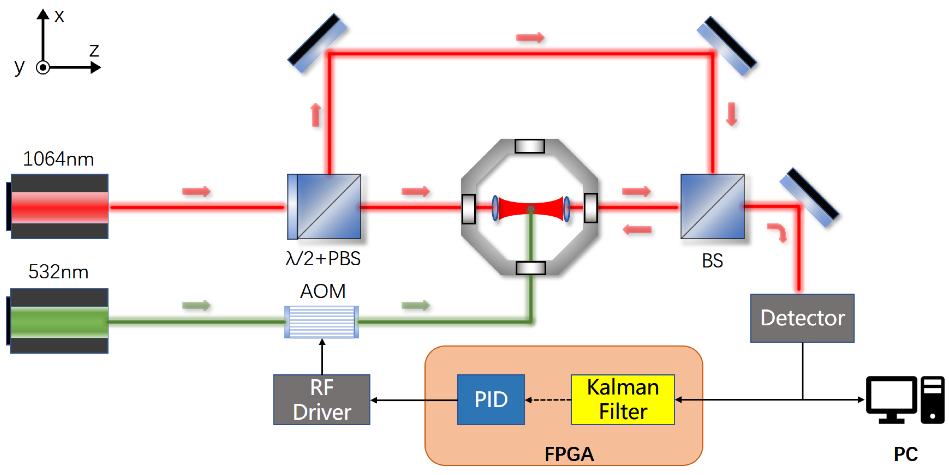
2.1. Counter-Propagating Dual-Beams Optical Trap

In a vacuum chamber, a silica spherical particle with a diameter of 10 μ m is restricted in a small area by two highly aligned and focused laser beams, which is known as an optical trap. The photodetectors collect the displacement information of the trapped particle from the center of the optical trap in the x, y, and z directions, which inevitably contains noise. This noisy measurement signal is processed using the Kalman filter and used as the input of a proportional-integral-derivative (PID) controller to generate a feedback signal, which drives the acoustic optical modulator (AOM) to modulate the light intensity of the cooling laser. The COM motion feedback cooling is realized via the damping effect of the modulated cooling light on the particle.
In our actual trapping system, the wavelength of trapping laser is 1064 nm, and the wavelength of the cooling laser is 532 nm. Both are continuous laser, and the power is always lower than 500 mW. The schematic of a single axis optical trap is shown in Figure 1.
Considering the structure of the optical trap, a spherical particle centroid should be on the axis of the beam in an ideal situation. However, it is difficult to achieve a well-aligned status in a dual-beam optical trap, which denotes the perfect coincidence of the focuses and optical axes of the dual-beams. The misalignment of the beams increases the trap stiffness nonlinearity and causes the particle to move in a larger area, affecting the detection accuracy and even increasing the risk of escaping.
Backward scattering detection is the most common method to detect displacement in an optical trap. This method uses photo-diodes to convert scattering light to voltage and then multiplies the differential voltage by the coefficient calibrated before the measurement to obtain the particle displacement. However, this detection method would inevitably bring the signal coupling effect to the optical trap with a microparticle, which is shown in Figure 2. The displacement power spectrum (PSD) of the particle, S, is a convenient tool to describe the particle motion amplitude of a certain frequency, as it is unnecessary to add devices of applying known forces into the trapping system and choosing the magnitude of the force carefully. In Figure 2, the radial detection signal is mixed with the radial signal at a frequency of about 800 Hz. As the range of motion in one direction increases, the coefficient in the opposite direction changes unexpectedly, resulting in single-axis signal distortion. Moreover, the total scattered light power collected by the radial detectors is strongly related to the axial position of the particle, intensifying the coupling effect. The coupling signal that occurs more often between the axial and radial signals causes an incorrect estimation of the particle motion mode and thus worsens the cooling performance, even heating the particle reversely. Therefore, to further stabilize and cool the particle’s motion, suppressing the noise and the coupling signal is critical.

2.2. System Model

In the microparticle optical trap, the particle’s motion mode can be simplified to a resonator for each axis independently when the particle is stably trapped near the equilibrium position of the optical trap. We assume that the levitated particle is only subjected to laser radiation pressure, random collision force of gas molecules, and the damping force of gas molecules and gravity and is unaffected by any other external forces. Additionally, all the forces have the same effect on the trapped particel in three directions except gravity. Hence, the Newtonian equation of motion of the COM of the particle on a certain axis can be expressed as follows:
M d 2 x d t 2 = k d i r G + F o p t ( t ) + F t h e r m ( t ) + F d r a g ( t ) ,
where M is the mass of the particle, x is the COM displacement of the particle, G = M g is the gravity on the particle and k d i r is the coefficient of G. The coefficient k d i r is 0 when we focus on the particle motion on the x-axis or z-axis, while it changes to 1 when we focus on the motion on y-axis.
F o p t is the force of laser radiation corresponding to the optical potential, which can be seen as proportional to the displacement in the submicrometer range for a microscale particle:
F o p t ( t ) = k · x ( t ) ,
where k is the trap stiffness of each axis. In counter-propagating dual-beam optical traps, the stiffness in x and y is similar and slightly higher than z.
F t h e r m is the random collision force of gas molecules on the particle, also known as the random fluctuation force. It is given as follows:
F t h e r m ( t ) = ζ ( t ) 2 k B T 0 γ ,
where ζ ( t ) is the normalized random noise with a mean value of zero in the time of t, k B is the Boltzmann constant, T 0 is the gas temperature around the particle and γ is the Stokes friction coefficient.
F d r a g is the drag resistance of the surrounding gas molecules on the particle and can be simplified as follows:
F d r a g ( t ) = γ v ,
where v is the velocity of the particle.
Combining the formulas above, we can describe the motion of the particle in a certain direction in the form of the Langevin equation:
x ¨ ( t ) + Γ 0 x ˙ ( t ) + Ω 2 x ( t ) k d i r g = Λ ζ ( t ) ,
where
Γ 0 = γ / M is the gas damping coefficient,
Ω = k / M denotes the eigenfrequency of the particle and
Λ = 2 k B T 0 Γ 0 / M follows the fluctuation dissipation theorem.
When we take the stiffness of common counter-propagating dual-beam optical traps and the mass of a micrometer particle into the formulas above, we can get that the eigenfrequency is at a kHz level. This is a big difference between micrometer particle traps and nanometer particle traps.

2.3. Kalman Filter

The Kalman filter, proposed by Rudolph E. Kalman in 1960, is an optimal recursive data processing algorithm. The basic principle of the Kalman filter is to weigh noisy observations and predictions obtained from the previous actual data and the state equation to estimate the actual state at the new moment. This algorithm is a recursive state space method in the time domain, and its discrete form can be conveniently implemented on a field-programmable gate array (FPGA), which is then used in a real-time detection system to extract the real motion information of the particle.
To change the form of the Kalman filter, we can rewrite Equation (5) as follows:
X ˙ ( t ) = A X ( t ) + w ( t ) ,
x ˜ ( t ) = H X ( t ) + v ( t ) ,
where X ( t ) = ( x ( t ) , x ˙ ( t ) ) T , x ( t ) is the particle displacement deviated from the center of the trap at time t, A = 0 1 Ω 2 Γ 0 is the state transition matrix and w ( t ) = 0 F t h e r m ( t ) / M + k d i r g T is the process noise, where g is the gravitational acceleration constant. The measured position of the particle is described by x ˜ ( t ) in Equation (7), H = 1 0 is the measurement matrix because the detectors could not get the velocity information of the particle, and v ( t ) is the noise induced during the measurement process, modeled as a Gaussian white noise process with the same noise power as the photodetector. To be more in line with the practical application situations, we obtain the discrete time system equations as follows:
X k + 1 = Φ X k + w k ,
x ˜ k = H X k + v k ,
where X k is the state vector (displacement, vector) at time t k , X k + 1 is that vector in the next moment t k + 1 , x ˜ k is the value obtained from the detectors at time t k , and w k and v k are the process and measurement noise signals following Gaussian distribution with covariance Q k and R, respectively. The state transform matrix Φ is given as follows:
Φ = e x p ( Γ 0 T s 2 ) · Γ 0 sin ( ω T s ) 2 ω + cos ( ω T s ) sin ( ω T s ) ω ( Γ 0 2 4 ω + ω ) sin ( ω T s ) Γ 0 sin ( ω T s ) 2 ω + cos ( ω T s ) ,
where T s = 1 / f s is the sampling period and ω = Ω 2 Γ 0 2 / 4 is the cyclic frequency of the underdamped oscillator [34]. Considering that the value of ω is always at a kHz level for microscale particles and the sampling rate is at a MHz level, then sin ( ω T S ) can be approximated as ω T s and cos ( ω T s ) can be approximated as 1 ω 2 T s 2 2 . In low-pressure conditions, Γ 0 T s is also small, so that the term e x p ( Γ 0 T s 2 ) can be approximated as 1. We obtain the simplfied matrix as follows:
Φ = 1 T s Ω 0 2 T s 1 Ω 2 T s 2 2 .
Using the state vector X ^ k 1 | k 1 at time t k 1 , the Kalman filter algorithm estimates the next state X ^ k | k 1 and prediction of a prior error covariance P k | k 1 at time t k as follows:
X ^ k | k 1 = Φ k 1 X ^ k 1 | k 1 ,
and a priory error covariance matrix as follows:
P k | k 1 = Φ k 1 P k 1 | k 1 Φ k 1 T + Q k ,
where Q k = T s 2 2 k B T 0 Γ 0 / M / 2 0 0 T s 2 k B T 0 Γ 0 / M is the predicted noise covariance matrix of the white noise process w k , and Φ k 1 is the state transform matrix at time t k 1 .
The optimal Kalman gain K k at time t k is then calculated as follows:
K k = P k | k 1 H T ( H P k | k 1 H T + R ) 1 ,
where x ˜ k is the particle displacement information obtained from the detectors, and R is the variance of detection noise. Then, we can obtain the state estimate X ^ k | k at time t k according to:
X ^ k | k = X ^ k | k 1 + K k ( x ˜ k H X ^ k | k 1 ) .
The final error covariance matrix is then given as follows:
P k | k = ( I K k H ) P k | k 1 ( I K k H ) T + K k R K k ,
where I is the identity matrix. After completing this formula, the next loop begins. Equations (12)–(16) is a complete recursive process of the Kalman filter, and obtaining the real signal only requires a step of calculation (Equation (15)) after obtaining the measured signal.

3. Simulation and Results

3.1. Simulink Setup

Based on the system model, Kalman filter theory and the actual active feedback cooling structure in Section 2, we build an optical trap simulation model of the particle motion as shown in Figure 3.
The model includes three main modules, namely, a particle motion module, detection module and feedback cooling module. We use three sub systems to independently describe the particle motion in three directions and synthesize the coupling signal to simulate the actual situation. After adding measurement noise to the detection module, we used the Kalman filter to process the signal and the processed signal was used as the input of the PID controller to generate feedback acceleration on the particle. The parameters of the simulation model are obtained from the experimental systems and are shown in Table 1. One significant feature of the microsphere is that the resonance frequency is as low as near 1 kHz compared with the nanoparticle, and we set the oscillation frequency of Ω z = 810 Hz, Ω x = 1200 Hz and Ω y = 1320 Hz as encountered in practice.

3.2. Results

First, we evaluate the noise suppression performance of the Kalman filter in a microscale optical trap. The time domain signal of the particle displacement in the direction of z in the optical trap is shown in Figure 4, where the blue line represents the real signal, the black line represents the signal after the detection module, and the red line represents the signal after Kalman filtering. The detection module adds some colored noise dominated by low frequencies in order to be close to the actual experimental environment. The root-mean-square error (RMSE) is the square root of the squared sum of the difference between the observed value from the true value and the ratio of the amount of data, which is used to measure the deviation between the observed and true values. It is given as follows:
R M S E = i = 1 N ( θ ^ i θ i ) 2 N ,
where θ ^ i is an estimator with respect to an estimated parameter θ i , and N is the amount of the data. Through the filtering process, the RMSE drops from 12.64 to 5.18 nm after filtering, indicating that the filtered data is more pure and trustworthy.
Considering the coupling situation, we added three axes signals with different weights to simulate the complex actual signal, as in Figure 2.
The coupled signal from the radial appears almost as high as the z-axis signal intensity in the z-axis detection signal. When we use this signal as the input of the PID controller to realize z-axis feedback cooling, as in the actual experiment, the motion amplitude in the axial resonance peak is suppressed. However, the particle’s motion is heated at the frequency of radial resonance peaks simultaneously because of the mixed coupling signals. To obtain the decoupled signal, we activate the Kalman filter, and the result is shown in Figure 5a, showing that the coupling peaks are effectively suppressed by 19.85 dB.
To confirm the behavior of the Kalman filter during the final step of the feedback cooling, we compared two simulation runs (with/without the Kalman filter), using the same feedback gain and PID controller coefficients, and outcomes are shown in Figure 5b. As expected, the z-axis motion of the particle at eigenfrequency is suppressed, but the particle is heated at the radial resonance frequency. The coupling signal severely obstructs the lowest temperature to which particles can be cooled, and if we only apply a single-axis feedback cooling to the particle, the phenomenon will be more obvious and troublesome because the other axes’ motions will not be restricted.
Considering that the conditions of each axis are different, we usually calculate the single-axis COM temperature T c . m . to evaluate the cooling performance and the status of the trapped particle as follows:
T c . m . = M Ω 2 x 2 k B ,
where x 2 is the variance of the particle position.
We simulated a process of cooling the particle motion in axial from room temperature (293 K), and the cooling result is 166.48 K without the Kalman filter and 121.45 K with the Kalman filter, with an improvement of approximately 27% at a pressure of 1 mBar. The results show that the Kalman filter system does work in the entire feedback cooling procedure, and the function of suppressing noise and signal coupling is satisfactory, solving the abovementioned problems and making a significant difference in the actual microscale particle cooling projects.

4. Discussion

Apart from the advantages described in the previous sections, using the filtered smooth signal to drive the derivative control may reduce the probability of the feedback value exceeding the set range. To implement the Kalman filter in a real experimental environment, the filter’s hyperparameters Q and R, the covariance of the process and measurement noise must be adjusted manually to adapt to different conditions. The time delay between the measured signal and Kalman filtered signal must also be calcined before practical application, which is proved to be interrelated to the resonance frequency [35], or else it will result in phase shifting and deteriorate the cooling performance. Another issue is that it is critical to precisely set the frequency parameter of the Kalman filter to the oscillation frequency of the particle [32], or even cause reverse heating, as seen in Figure 5b. We believe that this can be solved by providing an accurate real-time resonance peak measurement on FPGA chips to update the parameters of the filtering model in real-time while maintaining the operating frequency.
In this study, we verify the Kalman filter’s promising performance in vacuum optical traps, which could extract the real motion information from the noisy signals. This advantage could help cool the particle to a lower COM temperature and achieve a higher sensitivity in velocity and acceleration measurement. Cooling bigger particles to lower temperatures will also serve to facilitate the transition between macroscopic and microscopic substances. As for other motion modes, it also contributes to the understanding of the microscale particle spinning motion, which has reached a rotation speed of 5 GHz using a silica nanodumbbell with a diameter of 150 nm [36].
We think this could be successfully applied in other media, such as water solutions, because of its lower resonance frequencies. The more accurate signal after filtering will significantly help researchers learn the real state of the trapped particles or other biomolecules, which allows them to operate and analyze more correctly and rapidly.

5. Conclusions

Overall, the counter-propagating beam optical trapping method used for microscale particles in a vacuum is a promising technology. In this study, we use the Kalman filter in microparticle optical traps to suppress noise and decouple the axes’ mixed signal. The performance of the Kalman filter is verified using the Simulink model with parameters encountered in practice. At 1 mBar pressure, the RMSE reduces from 12.64 to 5.18 nm, the coupling signal peak is suppressed by 19.85 dB, and the ultimate cooling performance is improved by 27%. Compared to other decoupling methods, the Kalman filter has the advantage of easy adjustment as a digital filter algorithm and does not require changing the structure of the optical trap system. Therefore, we believe that this study will bring a new solution to the microparticle optical trap and contribute to achieving synchronous and accurate three-dimensional mechanical quantity measurements, in addition to cooling the particle to a lower temperature in the basic physics research field.

Author Contributions

Conceptualization, S.X. and H.H.; Data curation, S.X.; Formal analysis, S.X.; Funding acquisition, H.H.; Investigation, S.X., M.C. and J.Y.; Methodology, S.X.; Project administration, H.H.; Resources, J.Y.; Software, S.X.; Supervision, N.L.; Validation, S.X., X.C. and N.L.; Visualization, S.X.; Writing—Original draft, S.X.; Writing—Review & editing, X.C. and N.L. All authors have read and agreed to the published version of the manuscript.

Funding

This work was supported by the National Natural Science Foundation of China (No. 62075193), Zhejiang Provincial Natural Science, Foundation of China under Grant No. LD22F050002, Major Scientific Research Project of Zhejiang Lab, China (No. 2019MB0AD01) and National Program for Special Support of Top-Notch Young Professionals, China (No. W02070390).

Institutional Review Board Statement

Not applicable.

Informed Consent Statement

Not applicable.

Data Availability Statement

Not applicable.

Conflicts of Interest

The authors declare no conflict of interest.

Abbreviations

The following abbreviations are used in this manuscript:
COMCenter of Mass
PIDProportional Integral Derivative
AOMAcoustic Optical Modulator
RMSERoot Mean Square Error
FPGAField-programmable Gate Array

References

  1. Ashkin, A. Acceleration and Trapping of Particles by Radiation Pressure. Phys. Rev. Lett. 1970, 24, 156–159. [Google Scholar] [CrossRef]
  2. Kotnala, A.; DePaoli, D.; Gordon, R. Sensing nanoparticles using a double nanohole optical trap. Lab Chip 2013, 13, 4142–4146. [Google Scholar] [CrossRef]
  3. Gordon, R. Future Prospects for Biomolecular Trapping with Nanostructured Metals. ACS Photonics 2022, 9, 1127–1135. [Google Scholar] [CrossRef]
  4. Brunetti, G.; Sasanelli, N.; Armenise, M.N.; Ciminelli, C. Nanoscale Optical Trapping by Means of Dielectric Bowtie. Photonics 2022, 9, 425. [Google Scholar] [CrossRef]
  5. Shen, K.; Duan, Y.; Ju, P.; Xu, Z.; Chen, X.; Zhang, L.; Ahn, J.; Ni, X.; Li, T. On-chip optical levitation with a metalens in vacuum. Optica 2021, 8, 1359–1362. [Google Scholar] [CrossRef]
  6. Donato, M.G.; Patti, F.; Saija, R.; Iatì, M.A.; Gucciardi, P.G.; Pedaci, F.; Strangi, G.; Maragò, O.M. Improved backscattering detection in photonic force microscopy near dielectric surfaces with cylindrical vector beams. J. Quant. Spectrosc. Radiat. Transf. 2021, 258, 107381. [Google Scholar] [CrossRef]
  7. Bustamante, C.J.; Chemla, Y.R.; Liu, S.; Wang, M.D. Optical tweezers in single-molecule biophysics. Nat. Rev. Methods Primers 2021, 1, 1–29. [Google Scholar] [CrossRef]
  8. Peng, P.W.; Yang, J.C.; Colley, M.M.; Yang, T.S. An Optical Tweezers-Based Single-Cell Manipulation and Detection Platform for Probing Real-Time Cancer Cell Chemotaxis and Response to Tyrosine Kinase Inhibitor PD153035. Photonics 2021, 8, 533. [Google Scholar] [CrossRef]
  9. Lin, S.; Crozier, K.B. Trapping-Assisted Sensing of Particles and Proteins Using On-Chip Optical Microcavities. ACS Nano 2013, 7, 1725–1730. [Google Scholar] [CrossRef]
  10. Li, T.; Kheifets, S.; Medellin, D.; Raizen, M.G. Measurement of the Instantaneous Velocity of a Brownian Particle. Science 2010, 328, 1673–1675. [Google Scholar] [CrossRef] [Green Version]
  11. Li, T.; Kheifets, S.; Raizen, M.G. Millikelvin cooling of an optically trapped microsphere in vacuum. Nat. Phys. 2011, 7, 527–530. [Google Scholar] [CrossRef]
  12. Monteiro, F.; Li, W.; Afek, G.; Li, C.L.; Mossman, M.; Moore, D.C. Force and acceleration sensing with optically levitated nanogram masses at microkelvin temperatures. Phys. Rev. A 2020, 101, 053835. [Google Scholar] [CrossRef]
  13. Ranjit, G.; Atherton, D.P.; Stutz, J.H.; Cunningham, M.; Geraci, A.A. Attonewton force detection using microspheres in a dual-beam optical trap in high vacuum. Phys. Rev. A 2015, 91, 051805. [Google Scholar] [CrossRef]
  14. Ranjit, G.; Cunningham, M.; Casey, K.; Geraci, A.A. Zeptonewton force sensing with nanospheres in an optical lattice. Phys. Rev. A 2016, 93, 053801. [Google Scholar] [CrossRef]
  15. Rider, A.D.; Blakemore, C.P.; Gratta, G.; Moore, D.C. Single-beam dielectric-microsphere trapping with optical heterodyne detection. Phys. Rev. A 2018, 97, 013842. [Google Scholar] [CrossRef]
  16. Gonzalez-Ballestero, C.; Aspelmeyer, M.; Novotny, L.; Quidant, R.; Romero-Isart, O. Levitodynamics: Levitation and control of microscopic objects in vacuum. Science 2021, 374, eabg3027. [Google Scholar] [CrossRef]
  17. Volpe, G.; Maragò, O.M.; Rubinzstein-Dunlop, H.; Pesce, G.; Stilgoe, A.B.; Volpe, G.; Tkachenko, G.; Truong, V.G.; Chormaic, S.N.; Kalantarifard, F.; et al. Roadmap for Optical Tweezers. arXiv 2022, arXiv:2206.13789. [Google Scholar]
  18. Blakemore, C.P.; Fieguth, A.; Kawasaki, A.; Priel, N.; Martin, D.; Rider, A.D.; Wang, Q.; Gratta, G. Search for non-Newtonian interactions at micrometer scale with a levitated test mass. Phys. Rev. D 2021, 104, L061101. [Google Scholar] [CrossRef]
  19. Kawasaki, A.; Fieguth, A.; Priel, N.; Blakemore, C.P.; Martin, D.; Gratta, G. High sensitivity, levitated microsphere apparatus for short-distance force measurements. Rev. Sci. Instrum. 2020, 91, 083201. [Google Scholar] [CrossRef]
  20. Moore, D.C.; Geraci, A.A. Searching for new physics using optically levitated sensors. Quantum Sci. Technol. 2021, 6, 014008. [Google Scholar] [CrossRef]
  21. Carney, D.; Krnjaic, G.; Moore, D.C.; Regal, C.A.; Afek, G.; Bhave, S.; Brubaker, B.; Corbitt, T.; Cripe, J.; Crisosto, N.; et al. Mechanical quantum sensing in the search for dark matter. Quantum Sci. Technol. 2021, 6, 024002. [Google Scholar] [CrossRef]
  22. Taylor, M.A.; Bowen, W.P. A computational tool to characterize particle tracking measurements in optical tweezers. J. Opt. 2013, 15, 085701. [Google Scholar] [CrossRef]
  23. Zhu, X.; Li, N.; Yang, J.; Chen, X.; Hu, H. Displacement Detection Decoupling in Counter-Propagating Dual-Beams Optical Tweezers with Large-Sized Particle. Sensors 2020, 20, 4916. [Google Scholar] [CrossRef] [PubMed]
  24. Kalman, R.E. Contributions to the theory of optimal control. Bol. Soc. Mat. Mex. 1960, 5, 102–119. [Google Scholar]
  25. Kalman, R.E. A New Approach to Linear Filtering and Prediction Problems. J. Basic Eng. 1960, 82, 35–45. [Google Scholar] [CrossRef]
  26. Sandhu, F.; Selamat, H.; Alavi, S.; Mahalleh, V.B.S. FPGA-based implementation of Kalman filter for real-time estimation of tire velocity and acceleration. IEEE Sens. J. 2017, 17, 5749–5758. [Google Scholar] [CrossRef]
  27. Arroyo-Marioli, F.; Bullano, F.; Kucinskas, S.; Rondón-Moreno, C. Tracking R of COVID-19: A new real-time estimation using the Kalman filter. PLoS ONE 2021, 16, e0244474. [Google Scholar] [CrossRef]
  28. Li, Y.; Yin, G.; Zhuang, W.; Zhang, N.; Wang, J.; Geng, K. Compensating Delays and Noises in Motion Control of Autonomous Electric Vehicles by Using Deep Learning and Unscented Kalman Predictor. IEEE Trans. Syst. Man Cybern. Syst. 2020, 50, 4326–4338. [Google Scholar] [CrossRef]
  29. Wieczorek, W.; Hofer, S.G.; Hoelscher-Obermaier, J.; Riedinger, R.; Hammerer, K.; Aspelmeyer, M. Optimal State Estimation for Cavity Optomechanical Systems. Phys. Rev. Lett. 2015, 114, 223601. [Google Scholar] [CrossRef]
  30. Setter, A.; Toroš, M.; Ralph, J.; Ulbricht, H. Real-Time Kalman Filter: Cooling of an Optically Levitated Nanoparticle. Phys. Rev. A 2017, 97, 033822. [Google Scholar] [CrossRef]
  31. Jost, M.; Schaffner, M.; Magno, M.; Korb, M.; Benini, L.; Reimann, R.; Jain, V.; Grossi, M.; Militara, A.; Frimmer, M.; et al. An accurate system for optimal state estimation of a levitated nanoparticle. In Proceedings of the 2018 IEEE Sensors Applications Symposium (SAS), Seoul, Korea, 12–14 March 2018; pp. 1–6. [Google Scholar]
  32. Liao, J.; Jost, M.; Schaffner, M.; Magno, M.; Korb, M.; Benini, L.; Tebbenjohanns, F.; Reimann, R.; Jain, V.; Gross, M.; et al. FPGA Implementation of a Kalman-Based Motion Estimator for Levitated Nanoparticles. IEEE Trans. Instrum. Meas. 2019, 68, 2374–2386. [Google Scholar] [CrossRef]
  33. Magrini, L.; Rosenzweig, P.; Bach, C.; Deutschmann-Olek, A.; Hofer, S.G.; Hong, S.; Kiesel, N.; Kugi, A.; Aspelmeyer, M. Real-time optimal quantum control of mechanical motion at room temperature. Nature 2021, 595, 373–377. [Google Scholar] [CrossRef] [PubMed]
  34. Li, T. Fundamental Tests of Physics with Optically Trapped Microspheres; Springer: New York, NY, USA, 2013. [Google Scholar] [CrossRef]
  35. Zeng, X.; Zhang, B.; Han, X.; Chen, Z.; Xiong, W.; Chen, X.; Xiao, G.; Luo, H. Time delay remaining in the displacement detection of the optically trapped particles using Kalman filter. In Proceedings of the Third International Conference on Optoelectronic Science and Materials (ICOSM 2021), Hefei, China, 10–12 September 2021; Chen, S., Wang, P., Eds.; SPIE: Hefei, China, 2021; p. 13. [Google Scholar]
  36. Ahn, J.; Xu, Z.; Bang, J.; Ju, P.; Gao, X.; Li, T. Ultrasensitive torque detection with an optically levitated nanorotor. Nat. Nanotechnol. 2020, 15, 89–93. [Google Scholar] [CrossRef] [PubMed] [Green Version]
Figure 1. Schematic of trapping and feedback cooling in a vacuum optical trap. Only a single-axis detection and cooling system diagram is shown here.
Photonics 09 00700 g001
Figure 2. Coupling phenomena while trapping a 10 μ m-diameter sphere at 9.4 mBar in the experiment. The ordinate represents the root of three-dimension displacement power spectrum density of the particle. The red, green and blue lines represent the signals obtained from the detectors in the x, y and z directions, respectively. The dashed lines indicate that the fitted resonance peaks in three directions and the two radial resonant frequencies are close. The radial spectrum is only coupled seriously by axial signals and vice versa.
Photonics 09 00700 g002
Figure 3. The optical trap simulation model includes motion, detection and feedback cooling modules.
Photonics 09 00700 g003
Figure 4. The time domain signal of the particle displacement in the direction of z in the optical trap. The blue line represents the real motion of the particle, the black line represents the noisy signal after the detection module and the red line represents the signal processed by the Kalman filter.
Photonics 09 00700 g004
Figure 5. (a) The comparison of real signal, coupled signal and Kalman filtered signal. The ordinate represents the root of z-axis displacement power spectrum density of the particle. The blue line represents the real motion of the particle along the z-axis, the green line represents the z-axis detected signal mixed with the radial signal, and the red line represents the signal processed using the Kalman filter. The abscissa represents the frequency, and the ordinate represents the displacement power spectrum density. (b) The comparison of cooling performance using real signal, coupled signal and Kalman-filtered signal. The ordinate represents the root of z-axis displacement power spectrum density of the particle. The blue line represents the motion of the particle along the z-axis, the green line represents the particle motion in axial cooled using the coupled signal, and the red line represents the particle motion in axial cooled using the filtered signal.
Photonics 09 00700 g005
Table 1. Parameters of the optical trap simulation model.
System ParameterValue
Resonance frequency of z-axis ( Ω z ) 2 π × 810 Hz
Resonance frequency of x-axis ( Ω x ) 2 π × 1200 Hz
Resonance frequency of y-axis ( Ω y ) 2 π × 1320 Hz
Diameter (D)10 μ m
Density ( ρ ) 2.2 × 10 3 kg/m 3
Particle mass (M) 1.15 × 10 12 kg
Pressure (P)1 mBar
Damping ( Γ 0 ) 517.29 Hz
Sampling frequency ( f s ) 1 × 10 6 Hz
Publisher’s Note: MDPI stays neutral with regard to jurisdictional claims in published maps and institutional affiliations.

