Application of Visible Aquaphotomics for the Evaluation of Dissolved Chemical Concentrations in Aqueous Solutions

Abstract

This paper introduces novel research in aquaphotomics, extending the study of water–light interactions to the visible spectral range. This approach can potentially reduce the cost and increase the speed of spectral measurements, while providing additional information by extending the useful range in spectrophotometry. To demonstrate our method, we investigated the applicability of the visible spectral range for the quantification of NaCl dissolved in aqueous samples. Spectral measurements were conducted using a visible spectrometer in the range of 380–730 nm. The evaluation of molecular species concentration was based on multivariate analysis (MVA). Principal component analysis (PCA) showed a separation of all groups of samples by salt concentration. The partial least squares regression (PLSR) model presented high accuracy and a relationship between spectral variables in the visible range and NaCl concentration in water. The validity of the regression model was confirmed through independent prediction of NaCl concentration values in test samples with unknown concentrations. The presented results demonstrate the success of the approach in evaluating concentration changes in visible light, and thus extend the measurable spectral range of such analysis.

1. Introduction

In this paper, we extend the application of spectrophotometric and aquaphotomics methods into the visible range. Compared with classical near-infrared spectroscopy, the ability to detect changes in visible light is lower; however, the evaluation and interpretation using multivariate data analysis show statistically significant differences.

Spectrophotometry is one of the most useful methods for quantitative analysis in various fields. The novel method for the application of near-infrared spectroscopy, introduced by Professor Tsenkova in 2005, is called aquaphotomics, which has been successfully used to study and systematize the knowledge about water–light interactions [1,2]. The approach used in aquaphotomics is different from the traditional spectroscopy approach. In aquaphotomics, changes in the water spectral patterns are used as the main source of information, while classical spectroscopy methods only look for changes in the absorption of particular types of molecules. The change in the concentration of a particular analyte is reflected in the changes of absorbance at several water absorbance bands, which are then used to build the prediction model [3,4,5]. The majority of aquaphotomics studies have been done by near-infrared (NIR) spectroscopy [6,7,8,9,10].

A study of the mechanisms of light absorption by water molecules showed that there are overtones and combined vibrational absorption of water molecules in the visible range, resulting in six bands [11,12,13,14]. In the visible range, there are v1, v2 and v3 vibrational modes of O-H stretch, where v1 is symmetric stretch, v2 is bend (scissors mode), and v3 is asymmetric stretch; a and b are integers ≥0 and represent the order. The wavelengths of the peaks of the visible vibrational absorption spectrum of liquid water together with their assignments are presented in

Table 1. Assignment of the visible vibrational absorption spectrum of liquid water.

Wavelength	Assignment
739 nm	av1 + bv3; a + b = 4
660 nm	av1 + v2 + bv3; a + b = 4
606 nm	av1 + bv3; a + b = 5
514 nm	av1 + bv3; a + b = 6
449 nm	av1 + bv3; a + b =7
401 nm	av1 + bv3; a + b = 8

v1, v2 and v3 are vibrational modes of O-H stretch, where v1 is symmetric stretch, v2 is bend (scissors mode), and v3 is asymmetric stretch. a and b are integers ≥0 and represent the order.

. There is a small peak at 739 nm (av1 + bv3; a + b = 4), which corresponds to the third overtone band, plus a smaller fourth overtone band at 606 nm (av1 + bv3; a + b = 5), an extremely small fifth overtone band at 514 nm (av1 + bv3; a + b = 6), a seventh harmonic of the oxygen–hydrogen (OH) stretch at 449 nm (av1 + bv3; a + b = 7), an eighth harmonic of the OH stretch at 401 nm (av1 + bv3; a + b = 8), and a combined overtone band at 660 nm (av1 + v2 + bv3; a + b = 4) [15]. The absorption of overtone bands of water within the visible spectrum is quite small (0.3–0.01 m⁻¹), but never reaches exactly zero. The clear absorption of pure water without scattering effect was measured and examined by Pope and Fry in 1997 [16]. This research confirmed existing shoulders at 449 and 401 nm, which are due to the seventh and eighth harmonics of the OH stretch. The mentioned wavelengths represent the apexes of the water peaks; however, the changes of water absorption by dissolved chemicals affect water spectral pattern in total.

Based on this, it is assumed that the aquaphotomics approach can be applied in the visible range to determine information related to the higher water overtones. We examined the influence of the path length on the water spectral characteristics in the visible range of the spectrum [15] to choose an optimal technical path length and investigated the correlation between water spectral characteristics in the visible range [17] in our previous research. Using this knowledge, the current manuscript shows the accessibility of the visible range of the spectrum for the quantitative analysis of dissolved chemical in water.

Biological systems can be studied using a non-destructive and integrative approach based on aquaphotomics, i.e., the interaction between water and biomolecules in which spectroscopic techniques combined with multivariate analysis represent a powerful tool [3]. Near-infrared spectroscopy is successfully used for the quantitative analysis of many problems, including dissolved molecular species concentrations [18]. Visible aquaphotomics is proposed as a potential tool to increase the speed and reduce the cost of qualitative measurements. The aim of this study was to determine the application of visible spectroscopy and an aquaphotomics approach using an inexpensive spectrometer with a limited number of investigated bands to measure salt content in water.

2. Materials and Methods

2.1. Samples

Sodium chloride (NaCl, M = 58.44 g·mol⁻¹, purity min. 99.5% mass/mass) was purchased from Reanal (Budapest, Hungary). Purified water (MQ) was produced by a Milli-Q apparatus before the experiments (resistivity >18 MΩ·cm; Direct-Q, Millipore, Molsheim, France). Aqueous solutions were prepared from NaCl in a range between 2 and 20% w/v by direct dilution. First, stock solutions were prepared, and then they were further diluted with added MQ to reach the appropriate concentrations. This procedure was repeated three times to obtain three sets (repetitions) of samples, resulting in 30 samples of aqueous NaCl solution.

2.2. Spectral Acquisition

A ColorMunki (X-Rite) spectrophotometer was used to collect transflectance spectra. The ColorMunki works in the visible range (380–730 nm with steps of 10 nm = 36 wavelengths) and provides the measured spectrum in the form of relative intensity of each wavelength. Spectral acquisition was performed in transflectance mode using an optical glass window cuvette providing a 4.2 mm thickness of the tested sample (8.4 mm technical path length). As a holder we used reflectance cuvette from the instrument metriNIR (Figure 1). This cuvette has a circular shape and consists of a “bath” for the sample and a “head” with a reference white reflector.

The light passes through the glass located at the bottom of the cuvette, through the sample, is reflected from the white surface of the reflector, and returns back to the receiver. The thickness of the cuvette can be changed by using reflectors with different heights. The cuvette thickness was chosen based on the results of a previous experiment [15], where we measured the spectra of samples using a cuvette with changeable thickness. The path length has a strong influence on the absorption, and the groups of measured spectra with different path lengths are far from each other on the principal component analysis scatterplot (Figure 2). The longest path length shows the biggest variance due to poor repeatability [19]. The results with 4.2 mm cuvette thickness provided good repeatability together with sufficiently high values of useful signals.

All spectral acquisitions were performed at room temperature, and the temperature and humidity of the room were monitored using a Voltcraft DL-121TH Multi-Data logger to reveal any substantial environmental conditions.

Three consecutive scans were conducted for each measurement. Milli-Q water was measured between every 5 samples to detect the influence of environmental changes and device recalibration.

2.3. Statistical Data Analysis

For each sample, the reference spectrum was taken just before the measurement. As a reference, we used spectra measured from the white reflector.

Subtractive correction of environmental changes was applied. For this, from each sample’s spectrum we subtracted the spectrum of the pure Milli-Q water measured just before the set of 5 samples (EC_(i)) and added back the ground average spectrum of Milli-Q samples measured during the entire experiment calculated by the equation

$$E{C}_{avg}=\frac{1}{N}{\sum }_{i=1}^{N}E{C}_i,$$

(1)

where EC_avg is the calculated average of all relative intensities among whole Milli-Q water spectra measured during the experiment, and EC_i is the relative intensities among the Milli-Q water spectrum measured just before each set of 5 samples.

Then, subtractive correction of environmental changes can be presented as the equation

$$I_{c\left(i\right)}=I_{m\left(i\right)}-E{C}_{\left(i\right)}+E{C}_{avg},$$

(2)

where I_c(i) is the relative intensities after applying subtractive correction and I_m(i) is the measured relative intensities of the sample spectrum.

Relative absorption was calculated by the Lambert–Beer equation from the relative intensity provided by the ColorMunki spectrometer. For our data, we used the equation

$$A_{\left(i\right)}=lo{g}_{10}\left(\frac{I_{ref\left(i\right)}-I_{black}}{I_{c\left(i\right)}-I_{black}}\right),$$

(3)

where A_(i) is the calculated relative absorbance of the aqueous sample, I_ref(i) is the relative intensities among the measured spectrum of the white reference, I_black is the measured relative intensities with the totally closed spectrophotometer lens, used to avoid device error in the dataset, and I_c(i) is the measured relative intensities of the sample after applying subtractive correction.

To analyze the data, we used the Aquap2 R-studio package [20]. Data obtained during our experiment used for the analysis can be found in the supplementary materials in the form required by Aquap2 R-studio package: class- and numerical variables in Table S1 and measured spectral data (after applying the correction described above) in Table S2. In our experiments, the range of the spectrum from 380 to 730 nm was measured. To avoid the UV/VIS boundary region [21], we used only measurements above 410 nm for the processing. Analysis of the spectral range (420–730 nm) was done by following standard Aquaphotomics pipeline, including: inspection of the raw spectra first, principal component analysis, partial least squares regression model, and independent prediction by regression model.

Partial least squares regression (PLSR) models were used to predict NaCl concentrations based on the spectral characteristics of the aqueous samples. For the prediction, two separate PLSR models were built. The first model was calculated using all 90 measured spectra from 30 samples (three consecutive scans for each sample) to determine possible spectral outliers. The second model was calculated after removing the outliers (5 outliers were detected), using 85 measurements. To exclude outliers, the built-in function pls.exOut of the Aquap2 package was used. Outlier detection was performed by calculation of the boxplot for each of the PLSR predicted concentration level, and the points out of the 1.5 times the interquartile range from the median are identified as outliers. For both models it was decided to use three latent variables to minimize the chance of overfitting. Validation of both models was done by leave-one-out cross-validation, which means that three consecutive spectra of one sample were excluded from the training dataset at a time, the model was trained, then spectra of the next sample were excluded, and so on.

To simulate the use of the regression model in real conditions, which requires predicting the concentration of NaCl in solutions that were not previously presented to the model, independent prediction was used. For this purpose, the independent model was trained on two out of three repetition sets and tested on the third one.

The first inspection of the raw spectra showed possible grouping, as well as simple principal component analysis (PCA). Figure 3 shows the PCA scatterplot of aqueous samples with different NaCl concentrations. This example illustrates one repetition of samples with the same concentration range (Section 2.1) measured in the visible range (420–730 nm) using a cuvette providing 4.2 mm thickness. PCA successfully found a linear combination of the different spectral characteristics that separates out groups of aqueous solutions with different NaCl concentrations. The first two principal components show a clear trend. With an increased number of repetitions of each sample, the variance within each group grows, the groups do not appear well separated in lower dimensions, and it becomes necessary to use more principal components to cover the variance.

To obtain clear images, we preprocessed the dataset by standard methods (removing outliers, averaging, applying subtractive correction, and separating it into training and testing groups for modeling and validation).

3. Results and Discussion

The absorbance spectra of the tested aqueous solution of NaCl for the 420–730 nm spectral range are presented in Figure 4. Spectra are colored according to concentration, where a concentration of 0% is pure Milli-Q water. It can be observed that the changes in salt concentration give baseline shifts and wavelength-dependent variations.

PLSR models used for predicting NaCl concentration using all measured spectra and after removing the outliers are presented in Figure 5.

Cross-validation results of the models are presented in

Table 2. Performance of PLSR model developed for prediction of NaCl concentration in aqueous samples.

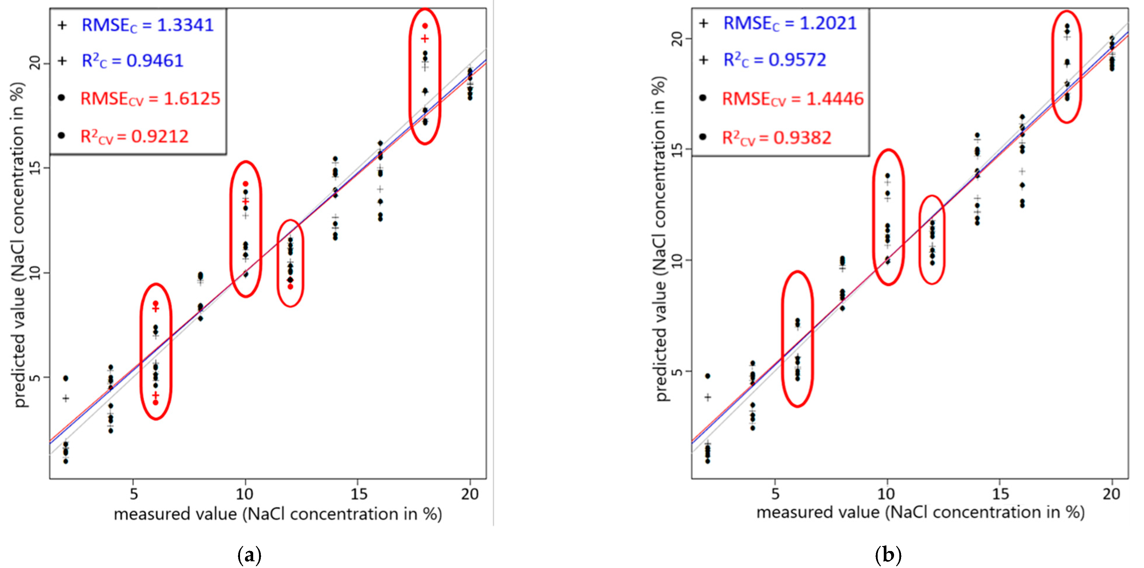
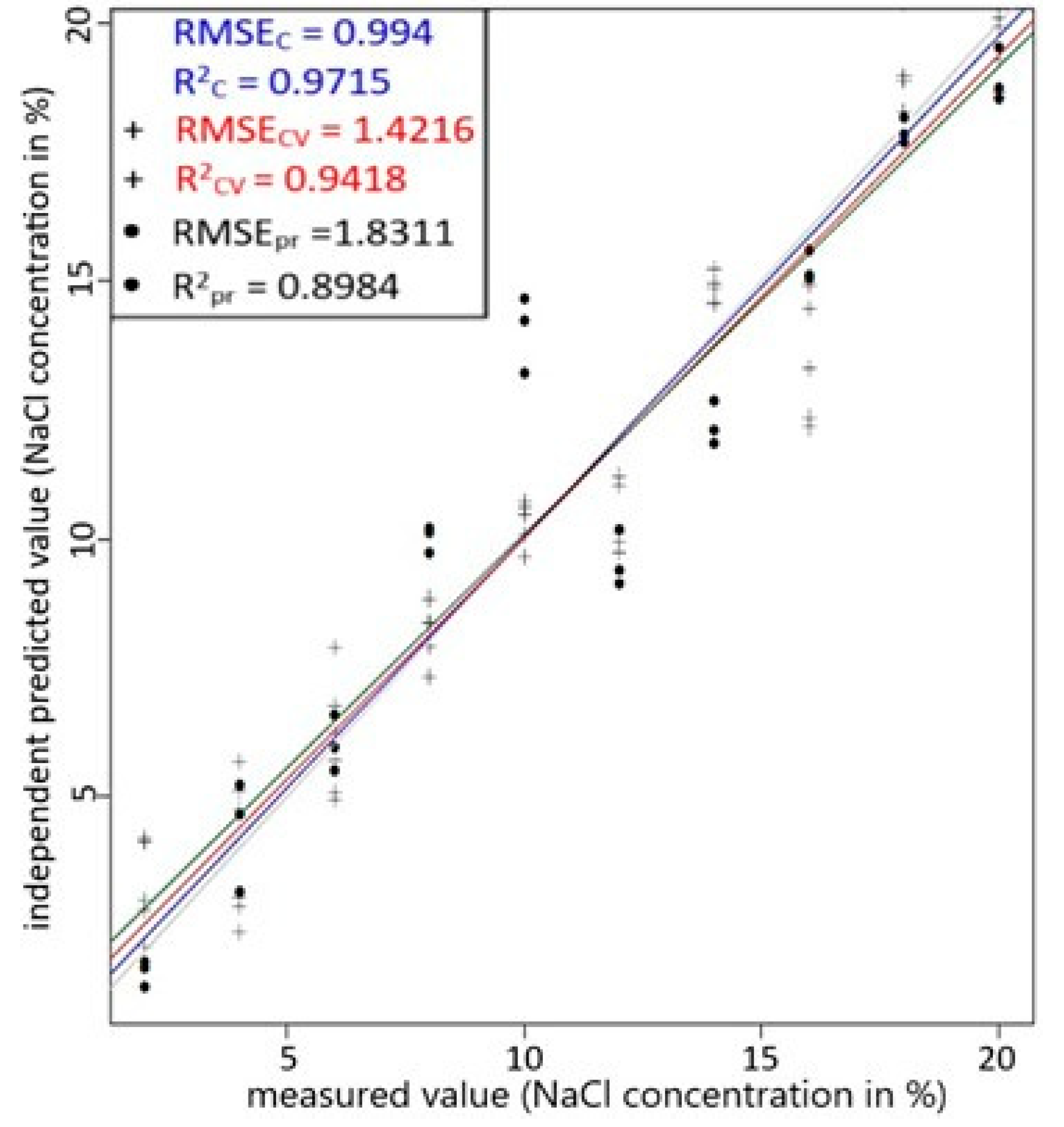
	Figure 5		Figure 6
	Model 1 (90 measurements)	Model 2 (85 measurements)	Model 1 (first set was used for testing)	Model 2 (second set was used for testing)	Model 3 (third set was used for testing)
Model calibration
R2C	0.95	0.96	0.97	0.96	0.95
RMSEC	1.33%	1.20%	0.99%	1.16%	1.29%
Cross-validation
R2CV	0.92	0.94	0.94	0.93	0.91
RMSECV	1.61%	1.44%	1.42%	1.52%	1.75%
Independent prediction
R2p			0.90	0.89	0.90
RMSEp			1.83%	1.91%	1.79%

. The coefficient of determination (R²) represents the accuracy of the model, and root-mean-square error of cross-validation (RMSE_CV) shows the precision of the cross-validation (minimal step in NaCl concentration, which can be accurately predicted by the model).

To validate the results of PLSR, the regression model was created with two groups (repetitions) of aqueous solutions and used to estimate the concentration of the third group, which had not been presented to the model before. After removing the outliers, three independent models were created in which the first group (Figure 6), second group (Figure S1), or third group (Figure S2) was used for the test. All of these models were trained separately, without presenting the test group. The results of cross-validation and independent prediction of models are presented in Table 2.

Regression analysis showed a strong relationship between spectral variables in the visible range and salt concentration in water according to the spectrometer with only 32 measured bands. This suggests the possibility of using the visible part of the spectrum for the analysis of some water parameters in specific tasks. This shows that the visible range of the water spectrum contains reasonable and useful information for qualitative analysis.

Our results demonstrate reasonable predictive accuracy compared with similar studies. For instance, Achata and colleagues [22] conducted a study to investigate hyperspectral imaging in the visible and near-infrared spectral ranges (450–1664 nm) coupled with chemometrics for the classification of brined and non-brined pork loins and prediction of brining salt (NaCl) concentration. They used brining solutions at concentrations of 5, 10, and 15% salt (w/v), prepared using vacuum-dried NaCl and distilled water. For the measurements, a hyperspectral imaging system in the visible–near-infrared range of 400–1000 nm with a spectral resolution of 5 nm was used. PLSR models were developed for the prediction of brine salt concentration. The PLSR model in the visible range (450–960 nm) obtained in that study with the highest R² and the lowest root-mean-squares error provided the following results: R²_C = 0.86, RMSE_C = 2.2% w/v, R²_CV = 0.84, RMSE_CV = 2.3% w/v, R²_p = 0.76, RMSE_p = 3.5% w/v. We are using shorter range, bigger step, therefore, smaller number of bands. The ColorMunki device, used in our experiment, measures spectrum in a range 380–730 nm with a step in 10 nm, resulting in 36 bands. Single measurement on this device takes around two-three seconds. Thus, we speed up the measurement process and decrease necessary computational burden. The possible limitation of our method is also related to the bigger measurable step, which could lead to losing some information. Nevertheless, the results presented in this article confirm the applicability of a smaller amount of measured data for the examination and prediction of molecular species concentrations dissolved in water.

4. Conclusions

Visible aquaphotomics performs quicker analysis, which reduces cost, and is easier to handle compared with the near-infrared approach. After previous attempts to investigate the accessibility of visible aquaphotomics, this paper presents the first reliable results showing the potential to expand the aquaphotomics approach to the visible range. Therefore, it is reasonable to more deeply investigate the information provided by the visible part of the spectrum. The next step is to expand the scope of the possible application of this method. The main question is to select or determine potential groups of dissolvable compounds distinguishable by the methods of visible aquaphotomics and evaluate the measurement precision and accuracy.

References

- Tsenkova, R. Visible-near infrared perturbation spectroscopy: Water in action seen as a source of information. In Proceedings of the 12th International Conference on Near-infrared Spectroscopy, Auckland, New Zealand, 9–15 April 2005. [Google Scholar]
- Tsenkova, R.; Muncan, J.; Pollner, B.; Kovacs, Z. Essentials of aquaphotomics and its chemometrics approaches. Front. Chem. 2018, 6, 363. [Google Scholar] [CrossRef] [PubMed]
- Muncan, J.; Tsenkova, R. Aquaphotomics—from innovative knowledge to integrative platform in science and technology. Molecules 2019, 24, 2742. [Google Scholar] [CrossRef] [PubMed] [Green Version]
- Chaplin, M. Do we underestimate the importance of water in cell biology? Nat. Rev. Mol. Cell Biol. 2006, 7, 861–866. [Google Scholar] [CrossRef] [PubMed]
- Tsenkova, R.; Iso, E.; Parker, M.; Fockenberg, C.; Okubo, M. Aquaphotomics: A NIRS investigation into the perturbation of water spectrum in an aqueous suspension of mesoscopic scale polystyrene spheres. In Proceedings of the 13th International Conference on Near-infrared Spectroscopy, Umea, Sweden, 17–21 June 2007. [Google Scholar]
- Weber, J.M. Isolating the spectroscopic signature of a hydration shell with the use of clusters: Superoxide tetrahydrate. Science 2000, 287, 2461–2463. [Google Scholar] [CrossRef] [PubMed]
- Weber, J.M.; Kelley, J.A.; Robertson, W.H.; Johnson, M.A. Hydration of a structured excess charge distribution: Infrared spectroscopy of the O2−⋅(H2O)n, (1⩽n⩽5) clusters. J. Chem. Phys. 2001, 114, 2698–2706. [Google Scholar] [CrossRef]
- Smith, J.D.; Cappa, C.D.; Wilson, K.R.; Cohen, R.C.; Geissler, P.L.; Saykally, R.J. Unified description of temperature-dependent hydrogen-bond rearrangements in liquid water. Proc. Natl. Acad. Sci. USA 2005, 102, 14171–14174. [Google Scholar] [CrossRef] [PubMed] [Green Version]
- Tsenkova, R. Aquaphotomics: Dynamic spectroscopy of aqueous and biological systems describes peculiarities of water. J. Near Infrared Spectrosc. 2009, 17, 303–313. [Google Scholar] [CrossRef]
- Tsenkova, R.; Kovacs, Z.; Kubota, Y. Aquaphotomics: Near infrared spectroscopy and water states in biological systems. In Membrane Hydration, 1st ed.; Disalvo, E., Ed.; Springer International Publishing: Cham, Switzerland, 2015; Volume 71, pp. 189–211. [Google Scholar] [CrossRef]
- Langford, V.S.; McKinley, A.J.; Quickenden, T.I. Temperature dependence of the visible-near-infrared absorption spectrum of liquid water. J. Phys. Chem. A 2001, 105, 8916–8921. [Google Scholar] [CrossRef]
- Chaplin, M. Water Structure and Science. Available online: http://www1.lsbu.ac.uk/water/water_structure_science.html (accessed on 3 August 2020).
- Yakovenko, A.A.; Yashin, V.A.; Kovalev, A.E.; Fesenko, E.E. Structure of the vibrational absorption spectra of water in the visible region. Biophys. Pergamon C C Biofiz. 2002, 47, 891–895. [Google Scholar]
- Walrafen, G.E.; Pugh, E. Raman combinations and stretching overtones from water, heavy water, and NaCl in water at shifts to ca. 7000 cm-1. J. Solut. Chem. 2004, 33, 81–97. [Google Scholar] [CrossRef]
- Bozhynov, V.; Mashchenko, O.; Urbanova, P.; Kovacs, Z. Steps to Visible Aquaphotomics. Lect. Notes Comput. Sci. 2020, 12108, 287–297. [Google Scholar] [CrossRef]
- Pope, R.M.; Fry, E.S. Absorption spectrum (380–700 nm) of pure water II integrating cavity measurements. Appl. Opt. 1997, 36, 8710–8723. [Google Scholar] [CrossRef] [PubMed]
- Bozhynov, V.; Soucek, P.; Barta, A.; Urbanova, P.; Bekkozhayeva, D. Dependency Model for Visible Aquaphotomics. Lect. Notes Comput. Sci. 2019, 11465, 105–115. [Google Scholar] [CrossRef]
- Lin, J.; Brown, C.W. Near-IR spectroscopic determination of NaCl in aqueous solution. Appl. Spectrosc. 1992, 46, 1809–1815. [Google Scholar] [CrossRef]
- Bozhynov, V.; Urban, J. Comparison of different types of error in visible aquaphotomics. In Proceeding of the 4th Aquaphotomics International Conference, Kobe, Japan, 20–22 March 2021; pp. 110–111. [Google Scholar]
- Pollner, B.; Kovacs, Z. Aquap2—Multivariate Data Analysis Tools for R Including Aquaphotomics Methods. Available online: https://github.com/bpollner/aquap2/ (accessed on 29 March 2021).
- Lawrence, K.P.; Douki, T.; Sarkany, R.P.E.; Acker, S.; Herzog, B.; Young, A.R. The UV/Visible radiation boundary region (385–405 nm) damages skin cells and induces “dark” cyclobutane pyrimidine dimers in human skin in vivo. Sci. Rep. 2018, 8, 12722. [Google Scholar] [CrossRef] [PubMed]
- Achata, E.M.; Inguglia, E.S.; Esquerre, C.A.; Tiwari, B.K.; O’Donnell, C.P. Evaluation of Vis-NIR hyperspectral imaging as a process analytical tool to classify brined pork samples and predict brining salt concentration. J. Food Eng. 2019, 246, 134–140. [Google Scholar] [CrossRef] [Green Version]