Spectral Output of Homogeneously Broadened Semiconductor Lasers

Abstract

Gain, spontaneous emission, and reflectance play important roles in setting the spectral output of homogeneously broadened lasers, such as semiconductor diode lasers. This paper provides a restricted-in-scope review of the steady-state spectral properties of semiconductor diode lasers. Analytic but transcendental solutions for a simplified set of equations for propagation of modes through a homogeneously broadened gain section are used to create a Fabry–Pérot model of a diode laser. This homogeneously broadened Fabry–Pérot model is used to explain the spectral output of diode lasers without the need for guiding-enhanced capture of spontaneous emission, population beating, or non-linear interactions. It is shown that the amount of spontaneous emission and resonant enhancement of the reflectance-gain (RG) product as embodied in the presented model explains the observed spectral output. The resonant enhancement is caused by intentional and unintentional internal scattering and external feedback.

1. Introduction

Gain is recognized as important in the operation of lasers, but gain is only one of the trio of gain, spontaneous emission, and reflectance that are important in the operation of lasers. This paper is a limited-in-scope review of the spectral output of homogeneously broadened semiconductor lasers. The review is limited to work on the spectral properties that the author was involved with. This work showed that the spectral output of a diode laser could be explained based on the reflectance-gain (RG) product and spontaneous emission as incorporated in a homogeneously broadened Fabry–Pérot model of a diode laser. It was not necessary to include population beating, non-linear interactions, or guiding-enhanced capture of spontaneous emission to explain the steady-state spectral output.

A simplified rate equation (or toy model) approach is used to describe the interaction of light and matter in a homogeneously broadened gain medium. Analytic but transcendental solutions for the single-pass gain and for the amplified spontaneous emission are presented for the coupled non-linear rate equations. These solutions are used in a Fabry–Pérot model of the output of a laser to understand the spectral output of homogeneously broadened lasers.

It is shown that the spectral output depends critically on the RG product and the amount of amplified spontaneous emission. The development of the mode sum/minimum method to estimate gain from spectrally resolved measurements is briefly mentioned. The effects of optical feedback and the effects of perturbations of the RG product by internal scattering centres on the steady-state spectral output are reviewed.

Rate equations, which typically are first order differential equations that keep track of populations and field intensities, are accurate descriptions of the amplification of light and saturation of populations provided that the dephasing caused by scattering or other processes is substantially faster than the natural relaxation rates of the interaction of light and matter ([1], Chapter 6).

III- V semiconductor lasers are thought to be homogeneously broadened. The intra-band relaxation time for carriers is of the order of 100 femtoseconds, which is the characteristic time for carriers to relax to an equilibrium distribution; the short time scale suggests that the quasi-Fermi level approximation is valid.

T. Mukai, K. Inoue, and T. Saitoh performed pump-probe measurements on $1.5\mathsf{\mu }$m InGaAsP travelling-wave semiconductor amplifiers [2]. They used a strong saturating signal on one wavelength and measured the gain on a weak probe as a function of wavelength. They found that the gain saturated homogeneously—that is, the gain saturated as

$$g\left(\nu \right)=\frac{g_o\left(\nu \right)S}{S+\int g\left(\nu \right)I\left(\nu \right)\mathrm{d}\nu }$$

(1)

where $g\left(\nu \right)$ is the gain at optical frequency $\nu$, $g_o\left(\nu \right)$ is the gain for input of a weak saturating signal, $\int g\left(\nu \right)I\left(\nu \right)d\nu$ is a weighted integral of the field intensity over all optical frequencies, and S is the saturation intensity.

M. P. Kesler and E. P. Ippen studied gain dynamics in AlGaAs diode amplifiers using 100 femtosecond optical pulses in a pump-probe set-up and found no evidence of spectral hole burning [3]. A two component recovery process with time constants of $\approx 300$ fs and 1.5 ps was observed. The faster process was postulated to be electron-hole thermalization and the slower process was postulated to be thermalization with the lattice.

E. O. Göbel et al. performed time and spectrally resolved measurements on an optically pumped ${\mathrm{Al}}_x{\mathrm{Ga}}_{1-x}\mathrm{As}$/GaAs double quantum well laser and found results that could be explained by homogeneous gain saturation [4]. At the highest pumping level, the entire spectral range, including the spontaneous emission, decayed with a time constant of $\approx 70$ ps, indicating that all carriers relax quickly to maintain a thermal distribution and recombine through the lasing channel. The researchers reported that no evidence of spectral hole burning was found.

E.I. Gordon, in his 1964 paper “Optical maser oscillators and noise” [5], noted that

“In an optical maser, gain saturation arises almost entirely from depletion of the population inversion, rather than from any nonlinearity in the stimulated emission process. To a very high degree, the output waveform is sinusoidal and the saturation depends only upon the time average power, the average extending over a time long compared to the period of the optical waveform, but short compared to any relaxation mechanism or pump rate.”

([5], p. 509)

Presumably Gordon pointed this out to contrast with the non-linear saturation required in a Van der Pol oscillator. The operation of a Van der Pol oscillator likely would have been understood by one of the target audiences of Gordon’s publication. Gordon derived, using a transmission line formalism, a Fabry–Pérot model of the spectral output of a laser. The work reported in [6,7] was influenced by Gordon’s publication.

In my experience, the spectral output of diode lasers can be explained, for the most part, by a homogeneously saturated Fabry–Pérot model, without the need to invoke non-linear mechanisms to explain deviations of the spectral envelope from smooth or without the need to invoke enhanced capture of spontaneous emission. The spectral output is set by the RG product and the amount of amplified spontaneous emission. Small perturbations in the reflectance, whether caused by internal reflections or scattering, or intentional or unintended external feedback, can have large effects on the steady-state spectral output.

The intent of this paper is to demonstrate this through a limited review of published work. First analytic solutions for mode intensities for propagation through a homogeneously broadened gain section are presented. Next, these solutions are used to complete a Fabry-P erot model of a diode laser. Finally, experimental results are presented to demonstrate the dependence of spectral output on the RG product and amplified spontaneous emission.

2. Homogeneously Broadened Gain

Consider a homogeneously broadened two-level system with a negligible population in the lower level. Let N represent the pumping rate per unit length into the upper level and let the natural lifetime, which is the lifetime in the absence of stimulated events, of the upper level represented by $\tau$. Assume counter propagating beams of light $I_i^{-}\left(z\right)$ and $I_i^{+}\left(z\right)$ with $I_i^{-}\left(z\right)$ propagating in the $-z$ direction and $I_i^{+}\left(z\right)$ in the $+z$ direction. Assume also that $I_i^{-}\left(z\right)$ and $I_i^{+}\left(z\right)$ interact with the population inversion with a strength denoted by ${\sigma }_i$. The subscripts ‘i’ are labels that denotes a mode, which includes a range of optical frequencies.

A rate equation for the inversion $n\left(z\right)$ at position z is

$$\frac{\mathrm{d}n\left(z\right)}{\mathrm{d}t}=N-\frac{n\left(z\right)}{\tau }-n\left(z\right)\sum _i{\sigma }_i\left(I_i^{-}\left(z\right)+I_i^{+}\left(z\right)\right)$$

(2)

with a steady state solution

$$n\left(z\right)=\frac{N}{S+{\sum }_i{\sigma }_i\left(I_i^{-}\left(z\right)+I_i^{+}\left(z\right)\right)}.$$

(3)

$S=1/\tau$ is the saturation intensity; the population inversion $n\left(z\right)$ begins to saturate when the rate of stimulated emission is comparable to the rate of transitions owing to spontaneous events.

Let the gain coefficient for the $i^{\mathrm{th}}$ mode be represented by $g_i$ and take ${\sigma }_i=g_i$. The equations can be solved analytically with ${\sigma }_i\ne g_i$, see Appendix A or [7], but set ${\sigma }_i=g_i$ for convenience. Assume a monomolecular recombination per unit length equal to $B_{i}n\left(z\right)$ into the optical frequency interval covered by the $i\mathrm{th}$ mode and assume no scattering or absorption loss [8]. Consequences of a constant lower level population for modelling a laser were considered in [9], and scattering loss was considered in [10]. It was found that a constant lower level population and scattering loss caused an increase of threshold and an increase of spontaneous emission relative to the case of no lower level population or no scattering loss. Both of these effects can be incorporated easily by appropriate scaling, and thus a laser model created by using the solutions of the equations retains relevance.

The assumptions above are idealizations that allow for an analytic solution. These idealizations retain homogeneously broadened effects and can be used to create a steady-state model that is useful for understanding the operation of a homogeneously broadened laser, particularly the spectral output and the effects of feedback on the steady-state spectral output.

Differential equations for propagation through a section of the gain medium are

$$\pm \frac{\mathrm{d}{I}_m^{\pm }\left(z\right)}{\mathrm{d}z}=\frac{g_{m}N{I}_m^{\pm }\left(z\right)+\beta B_{m}N}{S+{\sum }_i{g}_i(I_i^{-}\left(z\right)+I_i^{+}\left(z\right))}.$$

(4)

In the differential equations of Equation (4), the explicit expression for $n\left(z\right)$, Equation (3), has been used. Note that the the mode index m runs over as many modes as are necessary to describe adequately the problem. $\beta$ is the spontaneous emission factor and is a number that gives the fraction of the spontaneous emission that is captured by a mode [11]. For convenience, $\beta$ is assumed to be a constant across all modes, but, at the cost of another subscript $\beta$, can be allowed to be mode dependant.

Exact solutions to Equation (4) are given by [7,9]

$$I_m^{+}\left(L\right)=G_m{I}_m^{+}\left(0\right)+\frac{\beta B_m}{g_m}\left(G_m-1\right)$$

(5)

and

$$I_m^{-}\left(0\right)=G_m{I}_m^{-}\left(L\right)+\frac{\beta B_m}{g_m}\left(G_m-1\right).$$

(6)

$G_m$ is the single-pass gain for light in the $m^{\mathrm{th}}$ mode and for propagation in either the ‘+’ or ‘−’ directions, given inputs of $I_i^{+}\left(0\right)$ and $I_i^{-}\left(L\right)$ and outputs $I_i^{+}\left(L\right)$ and $I_i^{-}\left(0\right)$, where the index i runs over all modes and $L>0$. Steps to find Equations (5) and (6), the solutions to Equation (4), are given in Appendix A.

These solutions were found by trial and error, with paper and pencil, and with an unwavering belief over many pages and weeks of work that analytic solutions must exist. The solutions, which were found in 1983, can now be found using a symbolic processor in significantly less time that it takes to formulate the equations. Clearly it is worth the effort to become proficient with a symbolic processor.

For propagation in the ‘+’ direction, spontaneous emission that is produced close to $z=0$ travels further through the gain section and undergoes more amplification (or loss) than spontaneous emission that is produced close to $z=L$. The $(G_m-1)/g_m$ factor takes this into account [5]. Consider the simple case of exponential weighting of a constant $BN$ by distance from $z=0$ to $z=L$:

$$BN{\int }_0^{L}exp\left(gNL-gNz\right)\mathrm{d}z=B\frac{exp\left(gNL\right)-1}{g}=B\frac{G-1}{g},$$

(7)

which is the total amount of $BN$ detected at $z=L$ given an amplification of $exp\left[gN\right(L-z\left)\right]$ for a source of magnitude $BN\mathrm{d}z$ located at z. For small N, the total amount of $BN$ detected at $z=L$ is $BNL\times (1+gNL/2+O\left(N^2\right))$.

The single-pass gain is given by

$$G_m=exp\left[\frac{g_m\left\{NL-{\sum }_i\left[I_i^{+}\left(L\right)-I_i^{+}\left(0\right)+I_i^{-}\left(0\right)-I_i^{-}\left(L\right)\right]\right\}}{S-2{\sum }_i\beta B_i}\right].$$

(8)

Equation (8) indicates that the single-pass gain has an exponential dependence on $NL$ for small $I_i^{\pm }(·)$ and will saturate for $I_i^{\pm }(·)$ of order $NL$. The transcendental nature of Equations (5) and (6) is a consequence of the delicate balance that is explicit in the population inversion and field intensities for a homogeneously broadened medium. It helps to remember in Equations (5), (6) and (8) that $I_i^{-}\left(L\right)$ and $I_i^{+}\left(0\right)$ are the inputs to the gain section of length L and with pumping per unit length of N, and that $I_i^{+}\left(L\right)$ and $I_i^{-}\left(0\right)$ are the outputs of the gain section.

3. A Simple Fabry–Pérot Laser Model

A steady-state model for the output of a laser is presented in this section. If the expression for single-pass gain obtained in the previous section is used, then the model is a simplified model of a homogeneously broadened laser.

It is necessary to start with the electric field to include the resonator. Consider a monochromatic electric field $E^{\pm }(\nu ,z)$ where $\nu$ is the optical frequency of the electric field, z is the location, and ± indicates the direction of travel and ignore the polarization of the wave. The other independent polarization can be assigned to another mode and included in this manner. Assume reflectors at $z=0$ and $z=L$ with reflectivities $r_0$ at $z=0$ and $r_L$ at $z=L$. The electric field travelling in the ‘+’ at $z=0+ϵ$ where $ϵ$ is a vanishingly small positive number is $E^{+}(\nu ,0+ϵ)=r_0{E}^{-}(\nu ,0+ϵ)$.

At $z=L-ϵ$, the field travelling in the ‘+’ direction is $\sqrt{G}exp(-ikL)E^{+}(\nu ,ϵ)+{\delta }^{+}$, where ${\delta }^{\pm }$ is the total amount of spontaneous emission added to the field in crossing the cavity of length L in the ± direction and k is the magnitude of the wave vector. At $z=L-ϵ$, the field travelling in the ‘−’ direction is $r_L\left(\sqrt{G}exp(-ikL)E^{+}(\nu ,ϵ)+{\delta }^{+}\right)$. After propagating $E^{-}$ over a distance L, the field at $z=0+ϵ$ is $r_0{r}_{L}Gexp(-2ikL)E^{-}(\nu ,0+ϵ)+{\delta }^{-}+r_0{r}_L\sqrt{G}exp(-ikL){\delta }^{+}$. In steady state, the field must reproduce itself. Thus,

$$E^{-}(\nu ,0+ϵ)=\frac{{\delta }^{-}+r_L\sqrt{G}exp(-ikL){\delta }^{+}}{1-r_0{r}_{L}Gexp(-i2kL)}.$$

(9)

The detected intensity is $I^{\pm }(\nu ,z)=〈{\left|E^{\pm }(\nu ,z)\right|}^2〉$ where $〈·〉$ indicates a time average that is implicit in the detection process:

$$I^{-}(\nu ,0+ϵ)=\frac{〈{\left|{\delta }^{-}\right|}^2〉+R_{L}G〈{\left|{\delta }^{+}\right|}^2〉+\sqrt{R_{L}G}〈{\delta }^{-}{\delta }^{+*}+{\delta }^{-*}{\delta }^{+}〉}{{(1-\sqrt{R_0{R}_L}G)}^2+4\sqrt{R_0{R}_L}G{sin}^2\left(kL\right)}.$$

(10)

In Equation (10), the time independent phase of $exp(-ikL)$ has been absorbed into the spontaneous emission terms ${\delta }^{\pm }$. The superscript ${}^{*}$ means a complex conjugate.

It is tempting (and incorrect) to assume that the cross correlation $〈{\delta }^{-}{\delta }^{+*}+{\delta }^{-*}{\delta }^{+}〉=0$, since ${\delta }^{\pm }$ represent the spontaneous emissions in opposite directions and one could (incorrectly) imagine that the phases of ${\delta }^{-}$ and ${\delta }^{+}$ should be uncorrelated.

G. B. Morrison pointed out in his PhD work [12] that there are two indistinguishable paths for spontaneous emission from some point z, $0\le z\le L$, to reach an observer (take either ‘+’ or ‘−’ directions first and it is not possible to know which path was taken), and thus by the ‘rules’ of quantum mechanics, one must add these contributions coherently [13]. For $L\gg \lambda$, the coherent sum over all the multi-path contributions (${\delta }^{\pm }$ represent the sums over the length of the cavity of the spontaneous emission that is emitted in the ‘±’ directions) is negligible, and the cross correlation is essentially zero.

For gain-coupled DFB lasers, the contributions are regularly spaced and the effect of ignoring the coherent summation of contributions over indistinguishable multiple paths can be observed in the quality of fits to data—see Figure 7 of [13]. This coherent summation of the contributions of the spontaneous emission is probably the only quantum mechanical consideration that is necessary to model the laser. The concepts of stimulated emission, stimulated absorption, and spontaneous emission are explained classically [14].

The spectrally resolved output from the ‘0’ end is, then, $(1-R_0)\times I^{-}(\nu ,ϵ)$ assuming that the transmittance of the facet at $z=0$ is $T_0=1-R_0$. The output from the $z=L$ facet, $(1-R_L)\times I^{+}(\nu ,L-ϵ)$, can be found by interchange of the ‘0’ and ‘L’ subscripts and the ‘−’ and ‘+’ superscripts on the right-hand side of Equation (10).

The spectrally resolved output has peaks when ${sin}^2\left(kL\right)=0$ or when $kL=q\pi$ where q is an integer, $k=2\pi n_{r}L/\lambda$ is the magnitude of the wave vector, $n_r$ is the refractive index, and $\lambda$ is the wavelength in a vacuum. The spacing of the peaks (i.e., the free spectral range) in Hz is given by $c/\left(2n_{g}L\right)$ where $n_g$ is the group refractive index and c is the speed of light in vacuum. In terms of wavelengths, the free spectral range is $\Delta \lambda$ is ${\lambda }_1{\lambda }_2/\left(2n_{g}L\right)$ where ${\lambda }_1$ and ${\lambda }_2$ are the wavelengths of adjacent peaks.

By assuming knowledge of the product of the reflectances, $R_0{R}_L$, the single-pass gain G can be estimated as the ratio of the peak maximum to an adjacent minimum in the spectrally resolved output, which is the Hakki–Paoli method [15]. Otherwise, it is the $\sqrt{R_0{R}_L}G$ product that is determined from the spectrally resolved output.

The $m^{\mathrm{th}}$ mode intensity, where m is some convenient label, is determined by integrating the Airy function of Equation (10) over one free spectral range [5]:

$$I_m^{-}={\int }_{{\nu }_m-c/\left(4n_{r}L\right)}^{{\nu }_m+c/\left(4n_{r}L\right)}(1-R_0)\times I^{-}(\nu ,ϵ)\mathrm{d}\nu$$

(11)

with a corresponding definition for $I_m^{+}$. The longitudinal mode as defined by Equation (11) is correct in a quantum mechanical sense [16]. The longitudinal modes as defined include all optical frequencies. ${\nu }_m$ is the frequency that gives the peak intensity for the $m\mathrm{th}$ mode, i.e., the frequency for which $sin\left(kL\right)=0$ for mode m.

The $m\mathrm{th}$ mode intensity for output from the facet at $z=0$ is

$$I_m^{-}=\frac{\left(1-R_0\right)\times \beta B_m\times \left(G_m-1\right)/g_m\times \left(1+R_L{G}_m\right)}{1-R_0{R}_L{G}_m^2}.$$

(12)

The expression for $I_m^{-}$ was obtained by assuming the variables were constant over a free spectral range (or mode spacing) and identifying $|{\delta }^{\pm }{|}^2=\beta B_m\times (G_m-1)/g_m$. $B_m$ is the fraction of the total amount of spontaneous emission produced with optical frequencies that lie in the frequency interval defined by mode m, and $\beta$ is a geometric factor that gives the fraction of the spontaneous emission that is captured by the spatial mode [11].

$G_m$ is given by Equation (8), with $I_i^{+}\left(ϵ\right)=R_0{I}_i^{-}\left(ϵ\right)$ and $I_i^{-}(L-ϵ)=R_0{I}_i^{+}(L-ϵ)$. $I_m^{+}=(1-R_L)I_m^{+}(L-ϵ)$ and $I_m^{-}=(1-R_0)I_m^{-}\left(ϵ\right)$ since $I_m^{\pm }$ were defined as the output intensities and $G_m$ requires the internal intensities at the facets. The output intensities are not written with an explicit dependence on position (i.e., $I_m^{\pm }$), whereas the internal intensities are written with an explicit dependence on position (i.e., $I_m^{\pm }\left(z\right)$).

Equation (12) simplifies if $R_0=R_L=R$ since the denominator factors to $(1-R{G}_m)\times (1+R{G}_m)$ and the $(1+R{G}_m)$ terms in the numerator and in the denominator divide out.

The expression for $I_m^{-}$ (and the corresponding expression for $I_m^{+}$) are transcendental, since the mode intensities appear alone on the left-hand side of Equation (12) and in the exponential function $G_m$ on the right hand side of Equation (12). Despite this shortcoming and the simplifications made to derive analytic expressions, this model of a homogeneously broadened laser is useful for understanding the operation of a diode laser.

Some Asides

Equation (12) shows that a laser is a resonate amplifier of spontaneous emission [5]. The numerator of Equation (12) is amplified spontaneous emission whereas the denominator depends on the RG product, $\sqrt{R_0{R}_L}G$. A laser needs both gain and spontaneous emission. If $R_0=R_L=0$, then the output is simply amplified spontaneous emission. If $G_m<1$, then the output is attenuated spontaneous emission. For $G_m=1$, the gain medium is transparent.

It is often stated that $G_m=1/\sqrt{R_0{R}_L}$. From Equation (12) it is clear that, in steady-state operation, $G_m<1/\sqrt{R_0{R}_L}$ always. However, $G_m$ can be arbitrarily close to the limit (as in double precision close), particularly for high pumping rates and small quantities of spontaneous emission. What is not apparent from the equation for $I_m^{-}$ is that the amount of spontaneous emission affects the number of modes that contain an appreciable fraction of the output power.

The expressions for $I_m^{-}$ and $I_m^{+}$ can be used to obtain the ratio of the outputs from the two facets. For above-threshold operation, the approximation that $G_m=1/\sqrt{R_0{R}_L}$ can be used in the numerators (but not the denominators) to find the ratio of the outputs.

Equation (12) can be used to explain the dependence of the spectral output on facet coatings [17]. It is known that a laser with high facet reflectances operates more single-mode than the laser with low facet reflectances [18,19]. At threshold and beyond, the single-pass gain $G_m$ is larger for small $\sqrt{R_0{R}_L}$ than it is for larger $\sqrt{R_0{R}_L}$. Small $\sqrt{R_0{R}_L}$ corresponds to low facet reflectances. This means that the $G_m-1$ term in the numerator of Equation (12) will be larger for low facet reflectances than for high facet reflectances. A larger $G_m-1$ means more (amplified) spontaneous emission, and, all else being equal, a homogeneously broadened laser will operate more multimode with more spontaneous emission [17]. Unless specified otherwise, mode means the longitudinal mode.

Conventional wisdom asserts that homogeneously broadened lasers operate in single mode. This is true to a certain degree; however, a homogeneously broadened laser with a large numerator (i.e., a large amount of spontaneous emission) will run multimode. This fact is used in 980 nm pump modules to decrease the noise in fibre amplifiers by using incoherent feedback to cause multimode oscillation of a homogeneously broadened laser. Feedback into a laser that is incoherent with the field in the laser cavity is equivalent to increasing the amount of spontaneous emission in the laser and causes the laser to run more multimode [20,21]. Feedback that is coherent with the field in the laser cavity is equivalent to increasing the reflectivity of the facets [20] and makes the laser run more single-mode than without the feedback [17].

Consider a homogeneously broadened laser with $g_i={(1+i^2/2000)}^{-1}$ and $R_0=R_L=0.32$ for all modes. At twice threshold and for a particular choice of parameters, one finds, through simulation, that the mode at the gain peak, mode $i=0$, contains 94% of the total output power and that the modes adjacent to the gain peak, modes $i=\pm 1$, each contain 2% of the total power, for a side-mode suppression ratio (SMSR) of 48. For the same choice of parameters, except that the amount of spontaneous emission was increased by a factor of ten, mode $i=0$ contains 51% of the total power, and modes $\pm 1$ contain 15% each for a SMSR of $3.5$. Let only mode 0 receive feedback of ${10}^{-5}$ of the intensity in the cavity, which effectively changes $R_L$ for mode $i=0$ to $R_L=0.3236$.

Mode $i=0$ now contains $98.6\%$ or $86.3\%$ of the total power, for the two amounts of spontaneous emission, with SMSRs of 538 or 48. It is the amount of spontaneous emission and the RG product that determine the distribution of power amongst the modes. The amount of spontaneous emission sets the sharpness of the turn-on at threshold; see Figure 1 of [7].

The Hakki–Paoli method [15] to determine the gain of a laser is susceptible to contamination by the instrument response function of the instrument used to make the necessary spectrally resolved measurements. Equation (12) along with Equation (10) was used to create a method to estimate the gain of a laser, the mode sum/minimum or Cassidy method [22], which is tolerant of the spectral resolution of the instrument used to measure the spectrally resolved output. By using the mode power, which is integrating (or summing) the spectrally resolved output over a free spectral range of the cavity, the smoothing caused by the instrument response function is removed.

At the time, I knew that summing over independent measurements should improve the signal-to-noise ratio (if the noise was not $1/f$ noise) and that the mode sum would not be altered significantly by the convolution inherent in the measurement process. For a convolution, the area of a convolved function is the product of the areas of the two functions ([23], p. 118). The instrument response function should remain essentially the same over a region greater than the free spectral range of the laser cavity. Thus, the mode sum should not be altered significantly by the convolution inherent in the measurement process.

The only concern is that the mode is not isolated, and contributions from the adjacent modes will be included owing to the smearing (smoothing) caused by the instrument response function. This is true for both the Hakki–Paoli and mode sum/minimum methods. Provided that the parameters change slowly over a mode spacing, then the contributions from adjacent modes should not be significantly different than the mode of interest and both methods should give accurate results.

Nonlinear fitting to a convolution of Equation (12) produced low-noise estimates of the RG product of the laser from spectrally resolved measurement but was hampered for near- and above-threshold measurement by the broadened line shape of the Airy function [24]. The mode sum/minimum technique is not hampered by broadening of the Airy function.

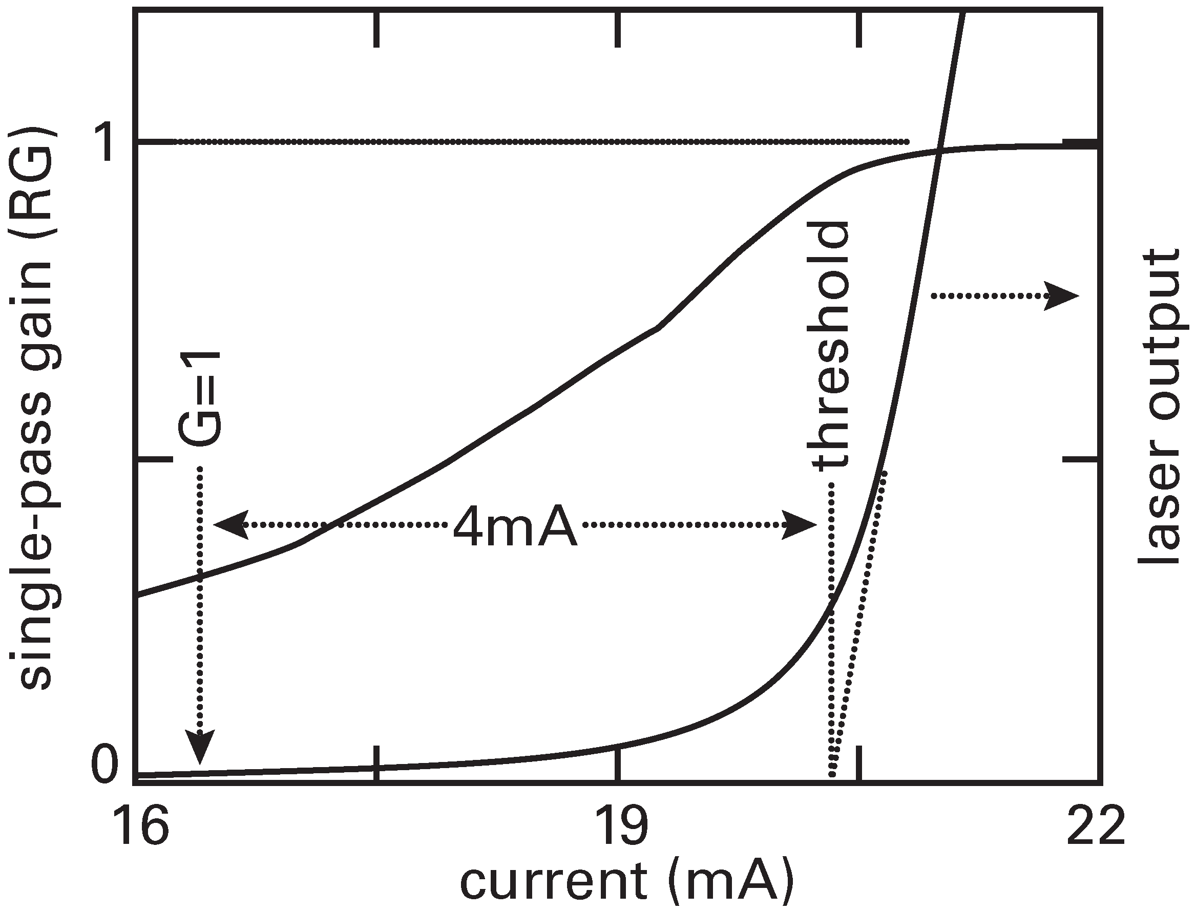
Equation (8) shows that the single-pass gain is exponential for small ${\sum }_i{I}_i^{\pm }(·)/S$ and saturates for large ${\sum }_i{I}_i^{\pm }(·)/S$. Figure 1, which displays the measured data, shows this behaviour. Additional examples of this exponential rise with pumping and saturation near and above threshold are shown in [6,22] and in Figure 5 of [7]. The mode sum/minimum technique was used to estimate the RG product from the measured spectrally resolved output [22].

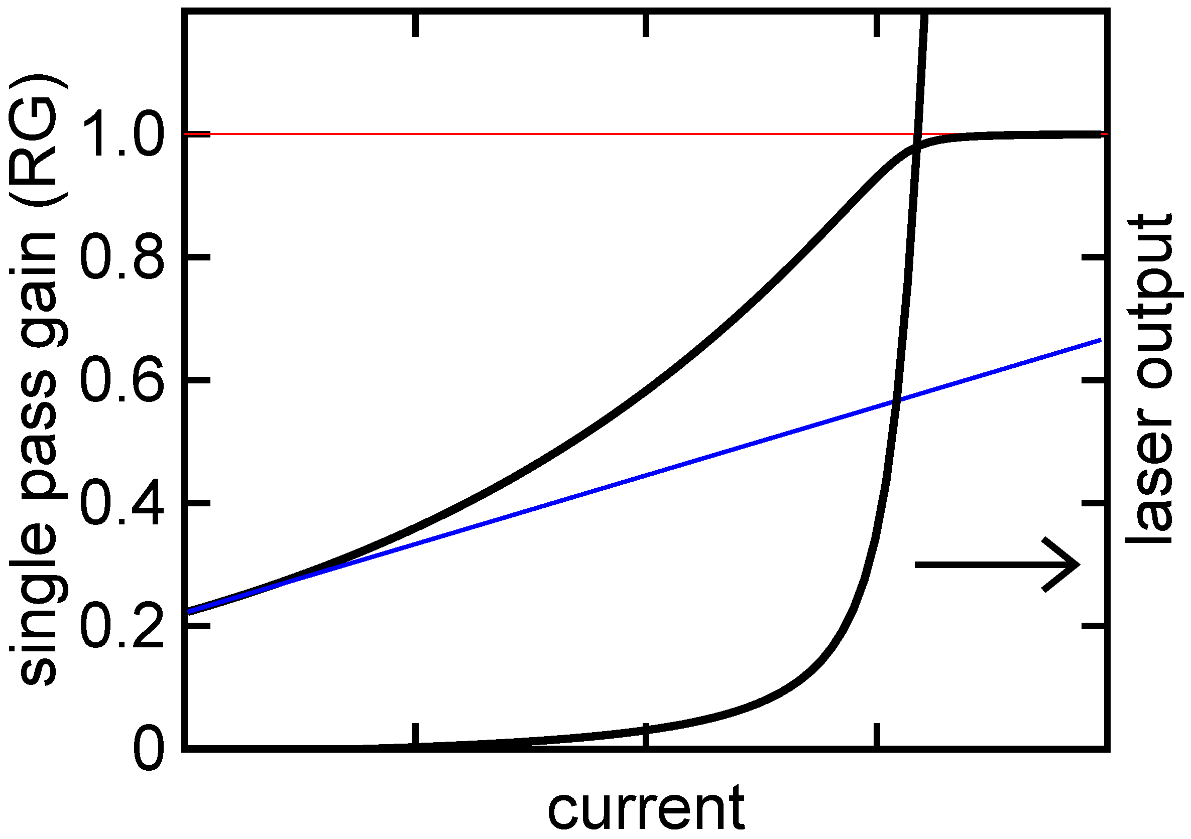
Figure 2 plots simulations of the single-pass gain and output power. The simulation parameters were chosen to provide a visual match to the measured data of Figure 1. The upward sloping line of Figure 2 is drawn to aid the reader. This straight line shows the exponential rise of the single-pass gain and the saturation near threshold. The total output power is also plotted in the figure. The single pass gain saturates at $0.9994$ for this selection of parameters. The horizontal line at RG equals unity is an asymptote that the single pass gain cannot reach.

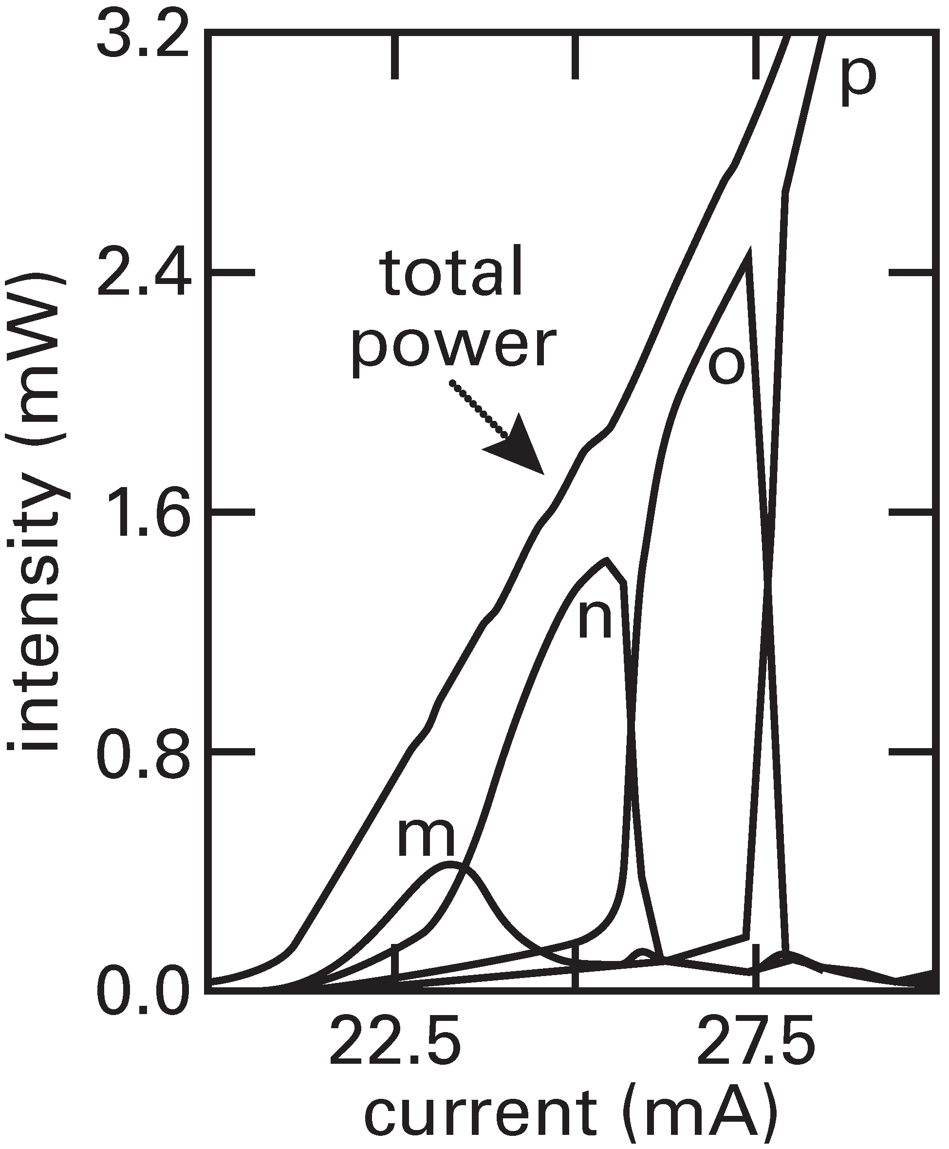
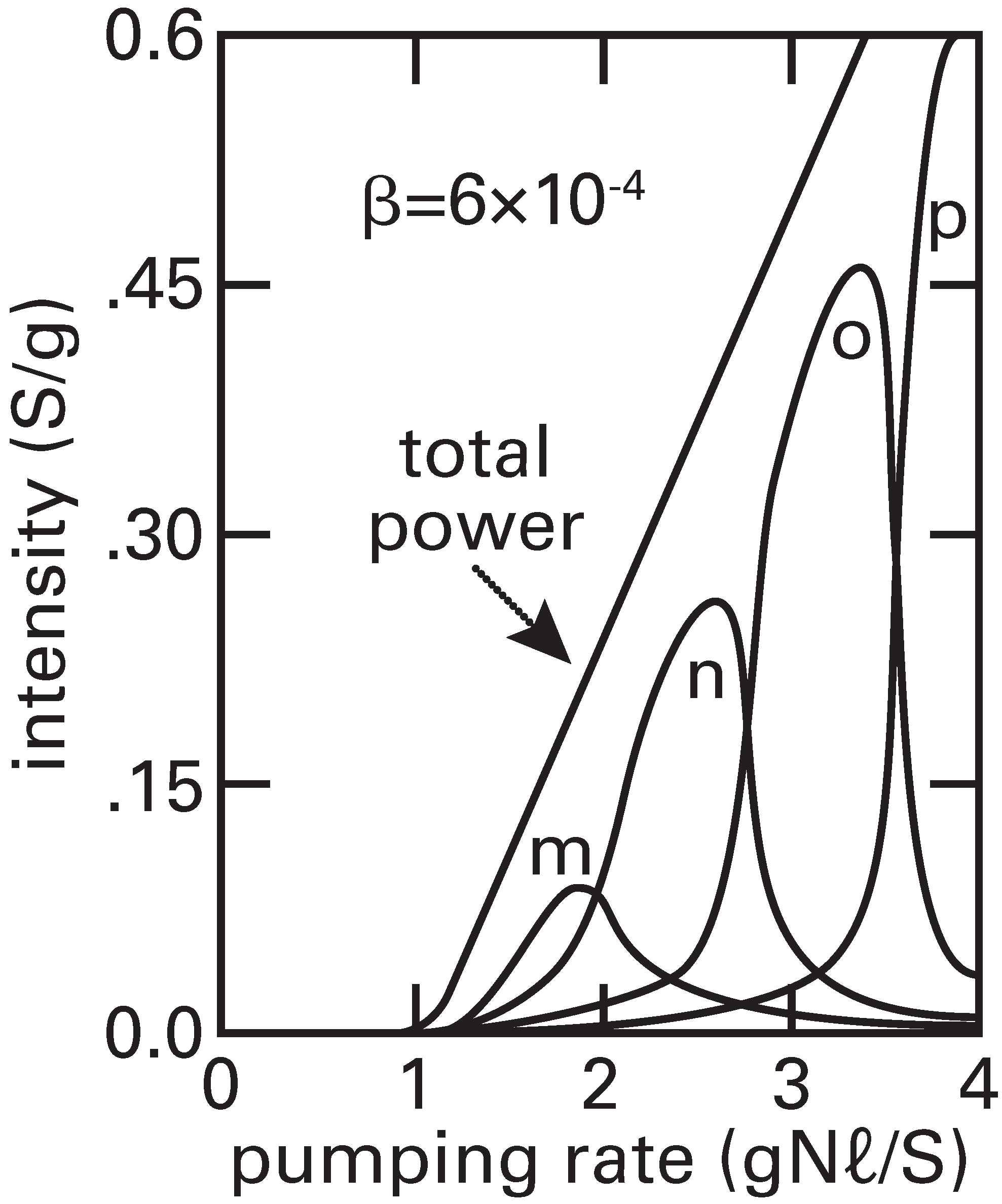
Figure 3 shows the total power and the power in the dominant modes as a function of current. The laser exhibits mode hopping owing to a red shift of the gain peak caused by ohmic heating of the active region. Figure 4 shows the output of a simulation that was matched to the data of Figure 3. The mode hopping was simulated by allowing the gain peak to be a linear function of the pumping rate. A comparison of the two figures reveals that the homogeneously broadened Fabry–Pérot model provides a realistic picture of the spectral output.

The usual approach to modelling the output of a laser is a rate equation approach [6]. Rate equations are written for the field intensity (usually called photon density; however, I side with the author of “Anti-Photon” [14] on this) and the population inversion. In steady state, the two equations are solved to yield a quadratic equation relating the field intensity and the pumping rate. There are several differences between the rate equation approach and the Fabry–Pérot approach [6].

The Fabry–Pérot approach explicitly includes the resonator; this ensures that the decay constant of the field intensity (i.e., ‘photon’ lifetime) is correct for small and large facet reflectances. In the Fabry–Pérot approach, the rate equation for the field intensity is integrated over the length of the gain section. In the rate equation approach, an infinitesimal that describes the interaction of light and inversion is taken to describe the interaction over the finite length L of the cavity. The rate equation approach does not allow for amplification of the spontaneous emission. This means that the rate equation approach cannot explain the change in spectral output for a change of facet reflectivity [17].

Owing to saturation from the homogeneous broadening, the two approaches will be forced (similar to a negative feedback forcing) to give similar looking output [6]. The rate equation approach gives a threshold, but the single-pass gain is linear and not exponential as shown in Figure 1 and Figure 2. In my opinion, a Fabry–Pérot approach to modelling a diode laser should be preferred.

4. Spectral Output

My graduate students and I used short external cavity (SXC) lasers for trace gas detection and spectroscopy applications. These SXC lasers were created by placing a planar mirror or a spherical mirror behind the rear facet. In an SXC configuration, single mode tuning in overlapping segments could be obtained. We used a 0.5-m monochromator retrofitted with a scanning mirror oscillating at ≳20 Hz to monitor the spectral output of the lasers on an oscilloscope in near realtime. The near realtime display meant that the effects of an SXC on the spectral output could be observed and verified easily.

L.J. Bonnell calculated that a planar mirror placed $\ell =160\mathsf{\mu }$m from a facet returned $\lesssim 4\times {10}^{-4}$ of the output power into the cavity. This small amount of feedback was sufficient to cause a laser that would normally operate multi-longitudinal mode to operate single-longitudinal mode, with a side-mode suppression-ratio of 0.1% ($-30$ dB) (Figure 2 of [25]). What was even more interesting was that this small amount of feedback caused a noticeable periodic modulation in the below-threshold spectral output (Figures 2–4 of [26]).

We could model the below-threshold and above-threshold spectral output of a SXC laser with a Fabry–Pérot model that included a wavelength dependant effective reflectance of $R_{eff}=R+{(1-R)}^2\tau R_{\ell }+2(1-R)\sqrt{R\tau R_{\ell }}cos(2k\ell )$ to account for the external cavity where R is the facet reflectance, $R_{\ell }$ is the reflectance of the external reflector a distance ℓ from the facet, and $\tau$ is the coupling efficiency. The coupling efficiency $\tau$ as a function of the angular alignment of the external cavity element was estimated by assuming Gaussian beam propagation and measuring the far fields to determine the Gaussian beam parameters [25].

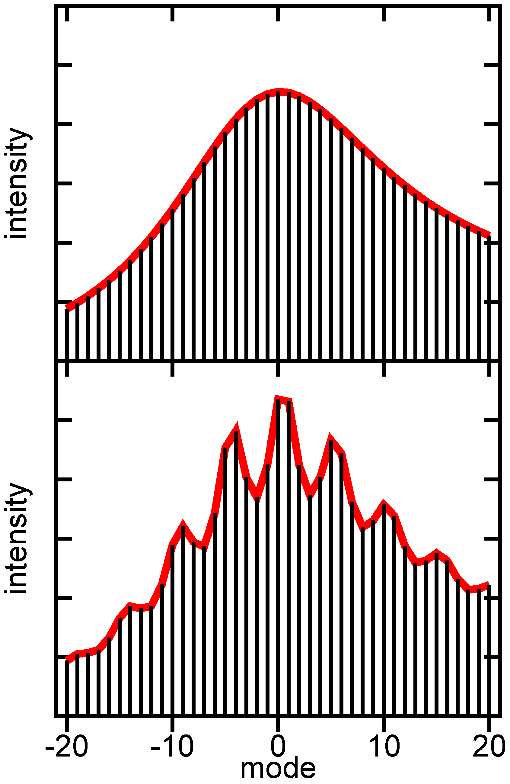
Figure 5 plots simulations of the below-threshold spectral output for a free-running laser (upper panel) and for a laser in an SXC. The length of the SXC, $\ell =160\mathsf{\mu }$m, and ${(1-R)}^2\tau R_{\ell }=1\times {10}^{-4}$ were chosen to match the measurements Figure 2 of the [25] and Figures 2–4 of the [26], which means that the phase of the feedback was adjusted to give roughly equal powers in mode ‘0’ and mode ‘1’. The modes are numbered consecutively with mode zero as the mode that had the maximum intensity and mode numbers increasing with decreasing wavelength.

A line, the spectral envelope, was drawn to connect the tops of the vertical lines that represent the intensity of the modes. The spectral envelope is smooth for the simulated free running laser and is modulated for the SXC laser. The depth of modulation scales with the amount of wavelength-dependent, coherent feedback; the greater the wavelength dependant feedback, the greater the modulation of the spectral envelope.

At the same time that L.J. Bonnell was developing SXC lasers for single mode tuning, F.H. Peters [27] was measuring the degree of polarization (DOP) of electroluminescence from the top of index-guided and gain-guided $1.3\mathsf{\mu }$m diode lasers [28,29,30,31,32,33,34]. Although the electroluminescence appeared uniform along the length of the lasers, the DOP of the luminescence was not uniform, and Peters identified the source of the non-uniformities in the detected DOP of luminescence as scattering.

This scattering had not previously been measured. From knowledge of the SXC work of Bonnell, we recognized that the scattering was of a magnitude to set (through modification of the RG product by resonate enhancement of selected modes) the spectral output of lasers. It was found that lasers with strong, discrete, internal scattering were more likely to operate single mode or with a strongly modulated spectral envelope than lasers with weak, discrete, internal scattering.

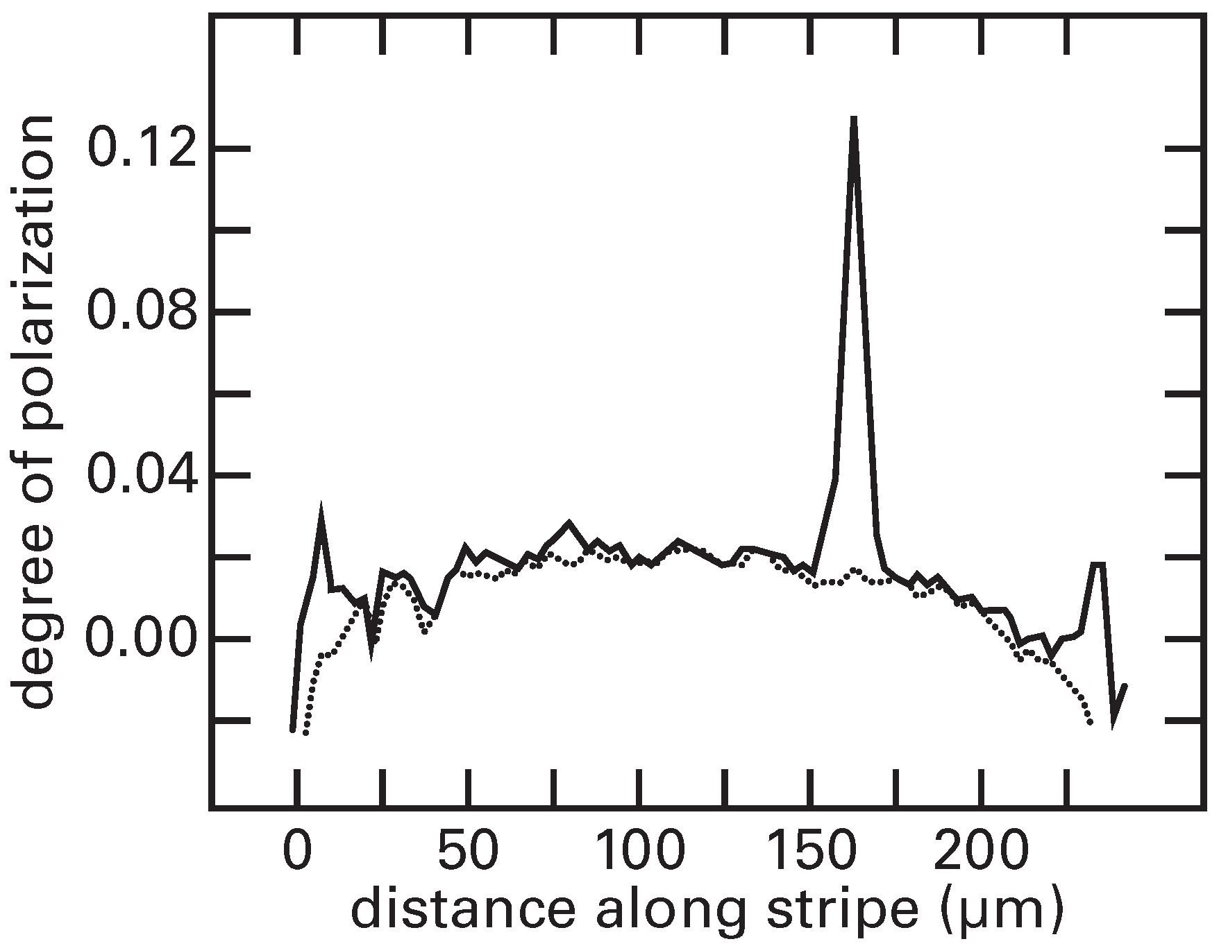
Figure 6 provides an example of what was identified as a scattering centre [30]. Electroluminescence that was propagating in a direction perpendicular to the plane of the active region, along a $\left[001\right]$ or z direction, was detected from lasers that had the top metal layers removed. The degree of polarization of this electroluminescence, $DO{P}_z$, was recorded, where

$$DO{P}_z=\frac{I_{\perp }-I_{\Vert }}{I_{\perp }+I_{\Vert }}$$

(13)

and $I_{\perp }$ is light polarized perpendicular to the stripe and in the plane of the active region, and $I_{\Vert }$ is light that is polarized parallel to the stripe. For below-threshold operations, $DO{P}_z\approx 0$ along the length of the stripe, as shown by the broken line in Figure 6. For above-threshold operation, lasers tended to show regions of large $DO{P}_z$, and these regions scaled with the output power. The direction of polarization for the perpendicular direction, ⊥, is the same as the direction of polarization for a TE lasing mode.

These regions of large $DO{P}_z$ for above-threshold operation were identified as scattering centres; light from the lasing TE mode was scattered into the detector for the perpendicular polarization. TM light could not scatter into the parallel, ‖, direction. The solid line in Figure 6 shows one strong scattering centre. The strength of the scattering centre could be estimated from measurements of the output power, the DOP signal, the collection efficiency of the DOP measurement system, and an assumption of Rayleigh scattering.

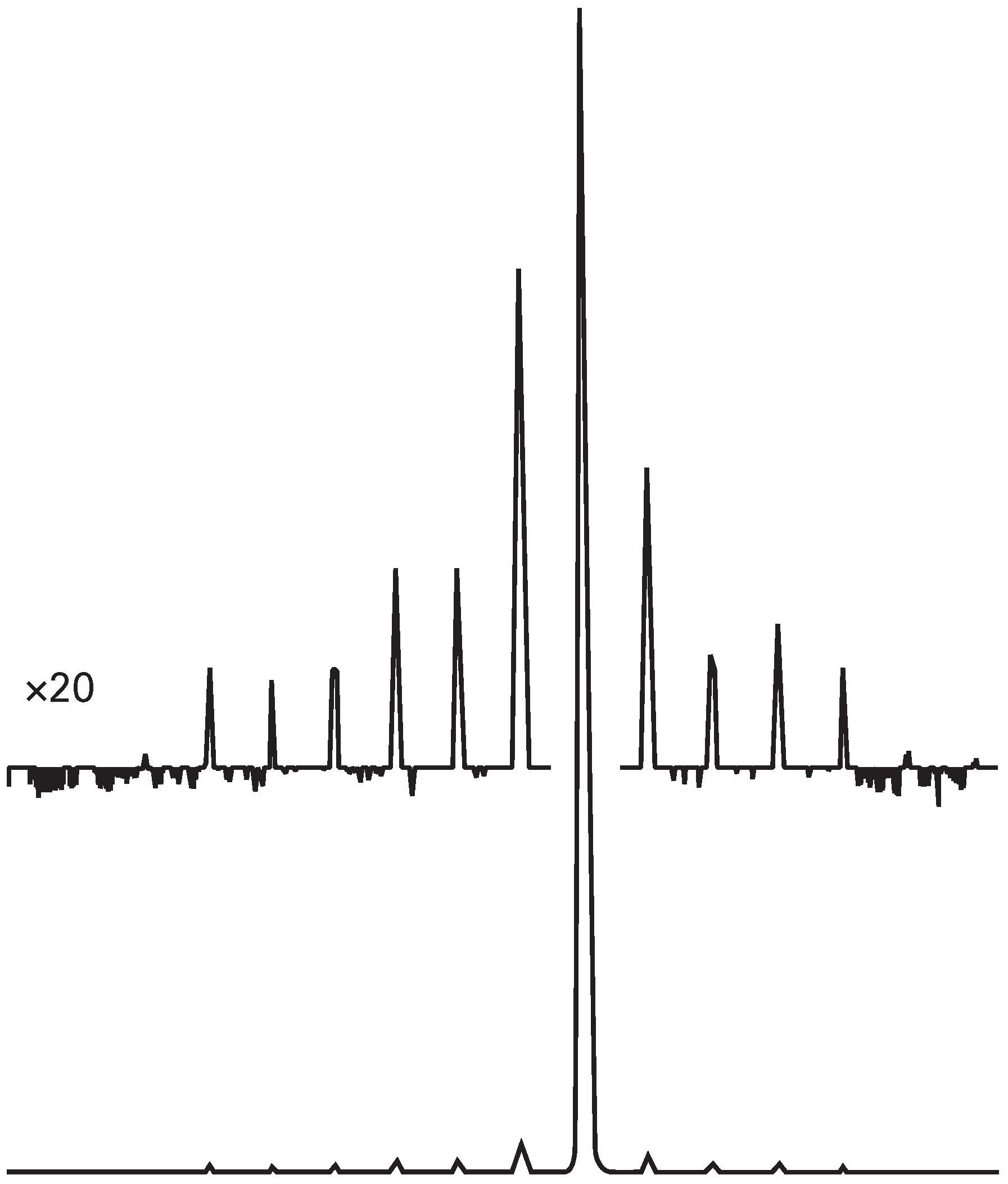
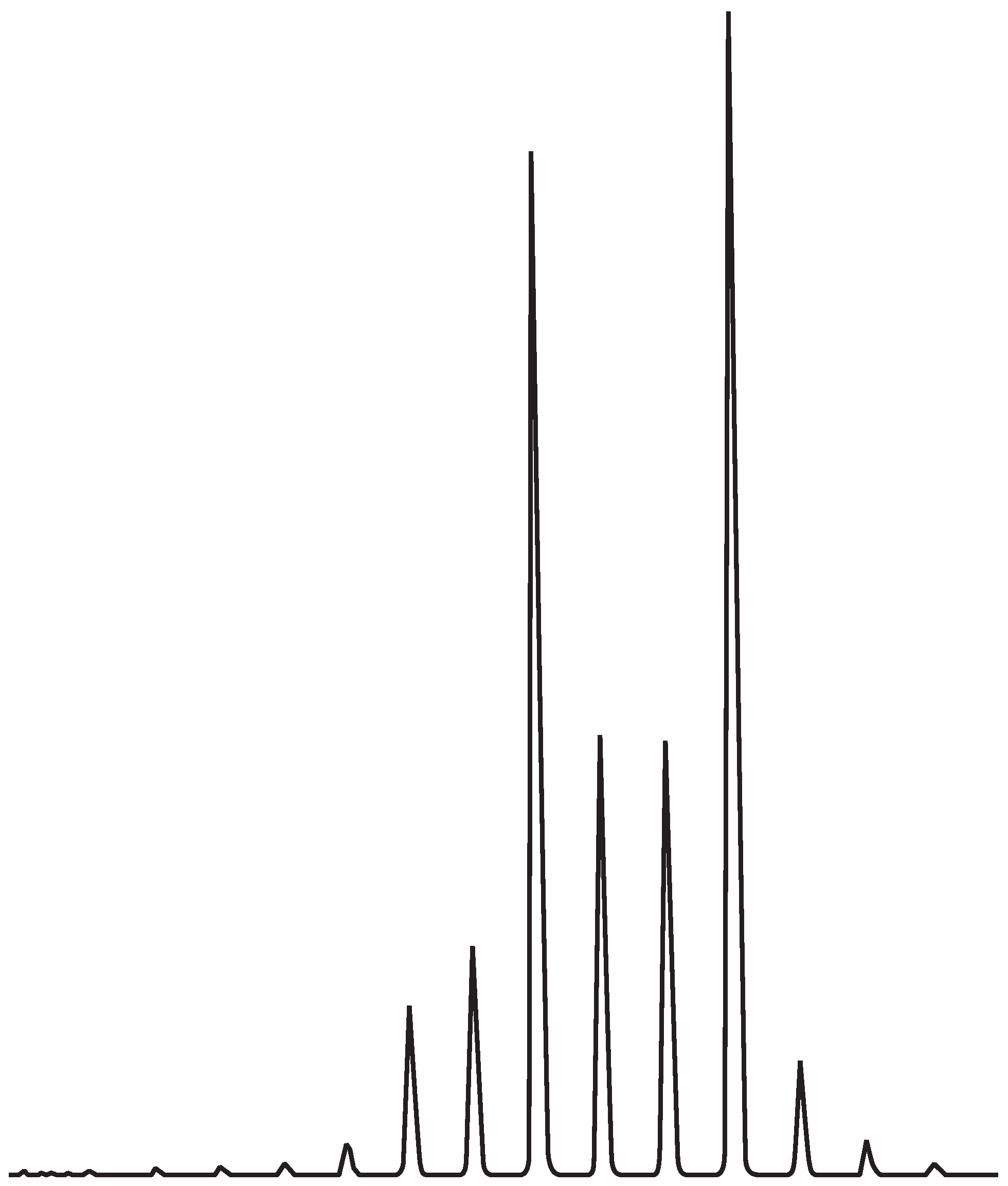
Figure 7 displays the spectral output for the device shown in Figure 6. Note the single-mode operation and modulation of the spectral envelope for this figure. This modulation is similar to the modulation of the spectral output for an SXC laser, an example of which is shown in Figure 5.

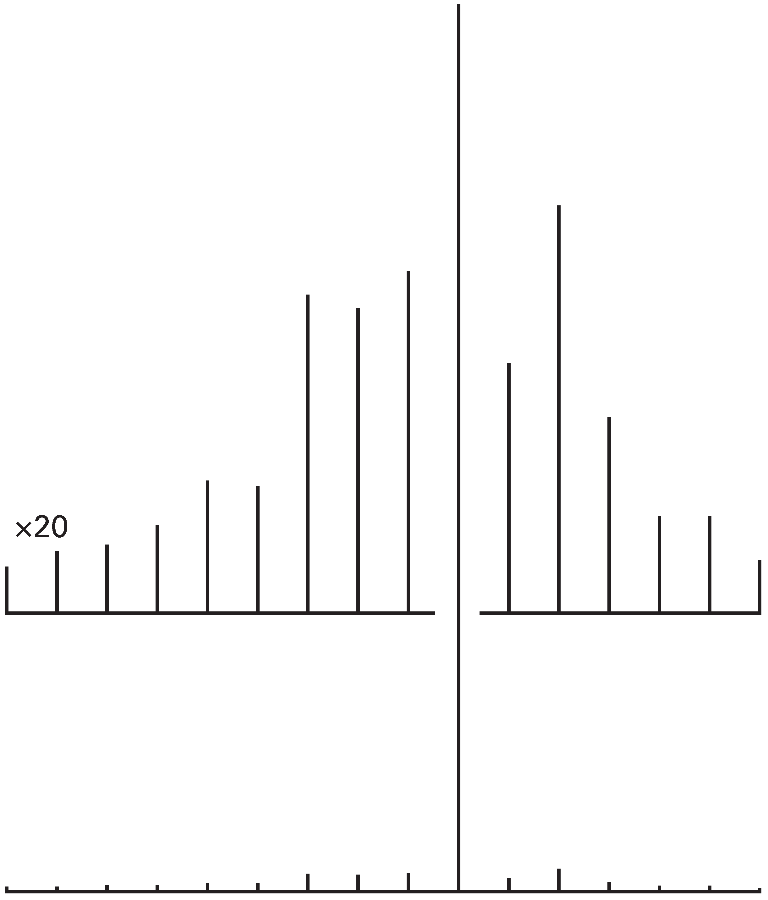
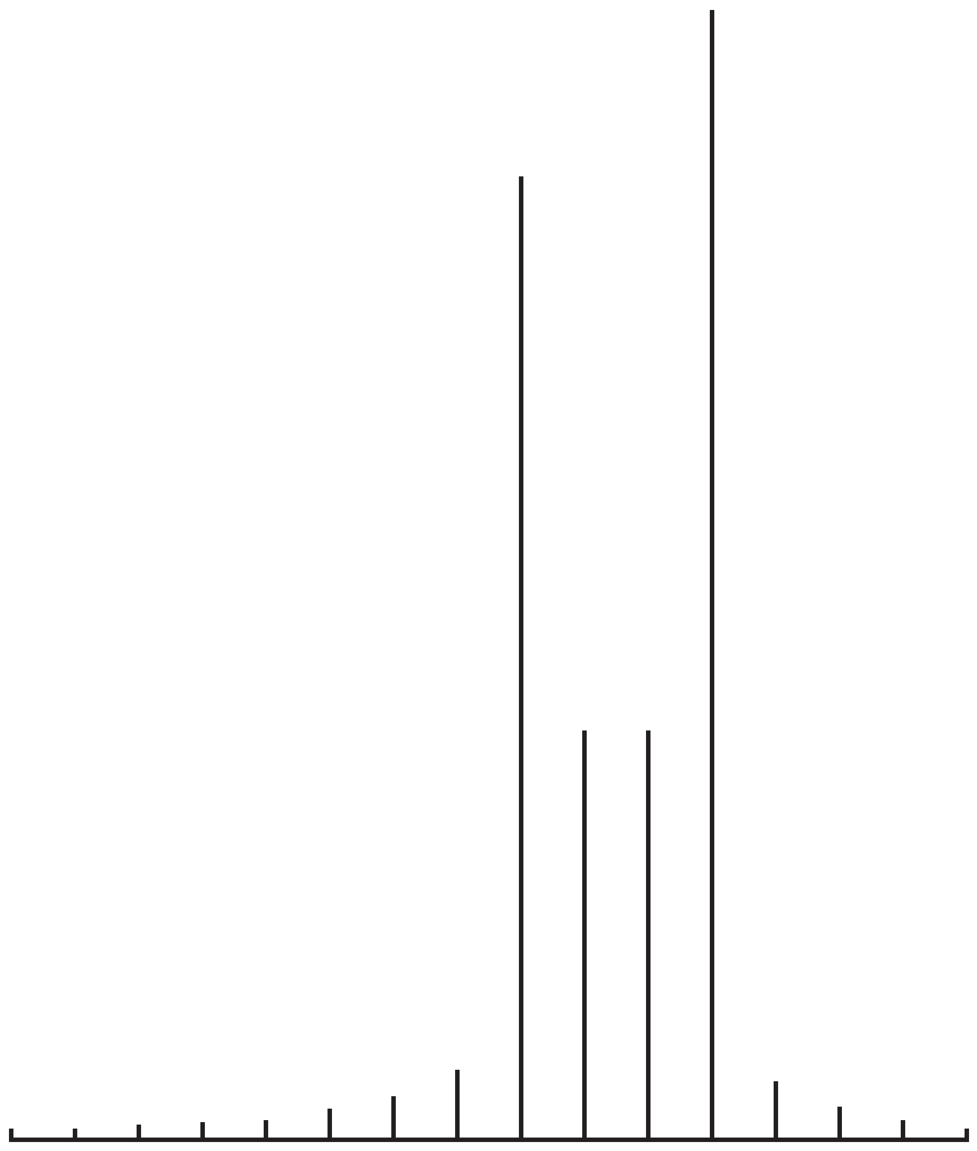
Figure 8 displays a simulated spectral output using effective reflectivity to model a scattering centre with the strength and location of the scatterer as determined from the measurements shown in Figure 6. The match between the features of the simulation and the measurement using experimentally determined scattering parameters for a single scattering centre is reasonable. Both the data and simulation show single-mode operation with modulation of the spectral envelope.

Figure 9 and Figure 10 provide another example of the fit between measured above-threshold spectral output of a laser and the simulated spectral output that used the scattering parameters obtained from $DO{P}_z$ measurements of the same laser. The so-called ‘double gain-peak’ behaviour is seen to arise from resonant enhancement of the RG product and not from two distinct gain peaks.

In addition to explaining spectral outputs based on scattering parameters of the lasers, the difference in spectral properties of index-guided and gain-guided lasers was explained. Index-guided lasers tended to run more single mode than gain-guided lasers. Gain-guided lasers have significantly larger threshold currents than index guided lasers, and this means that gain-guided lasers have larger amounts of spontaneous emission coupled into the modes than index guided lasers. The large amount of spontaneous emission leaves gain-guided less susceptible to scattering centres than lower threshold index-guided lasers [33]. In addition, for the lasers that we tested, the gain-guided lasers showed less scattering than the index guided lasers [31].

Some of the lasers that Peters examined were found to tune backwards; the lasing mode would shift to shorter wavelengths over a limited range of current. This anomalous tuning could be explained by the existence of multiple scattering centres and local heating caused by absorption [34]. J.E. Hayward [35] measured and analyzed the below-threshold and above-threshold spectral output of >30 diode lasers and was able to correlate the above-threshold spectral output with the degree of modulation of the below-threshold spectral envelope [36,37]. He calculated the RG product for ≈30 modes using the mode sum/minimum technique and fitted the RG values to a smooth curve to extract a residue.

He also captured the extremes in the above-threshold output—most single-mode and most multi-mode—over a range of currents and temperatures (from threshold to twice threshold and from 25 °C to 35 °C, to sample the spectra over a range of conditions), and computed a statistic Z to characterize the shapes of the extremes of the above-threshold spectral output [37]. The rms value of the residue, $\chi$, was found to be correlated with the value of Z. Lasers with smooth below-threshold spectral envelopes operated more multimode than lasers with modulated below-threshold spectral envelopes. The correlation was strengthened when the amount of spontaneous emission in the modes was included in the analysis.

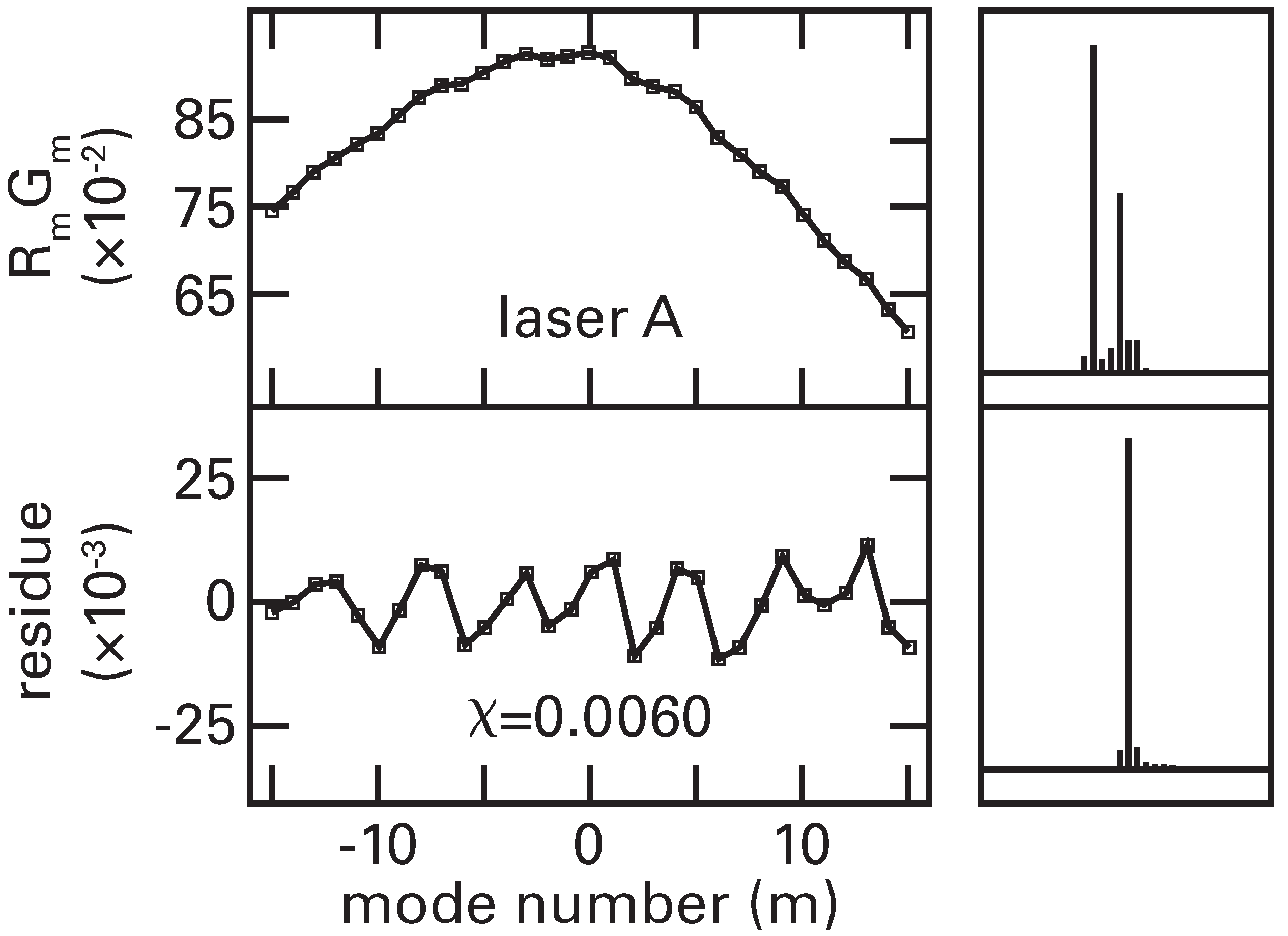
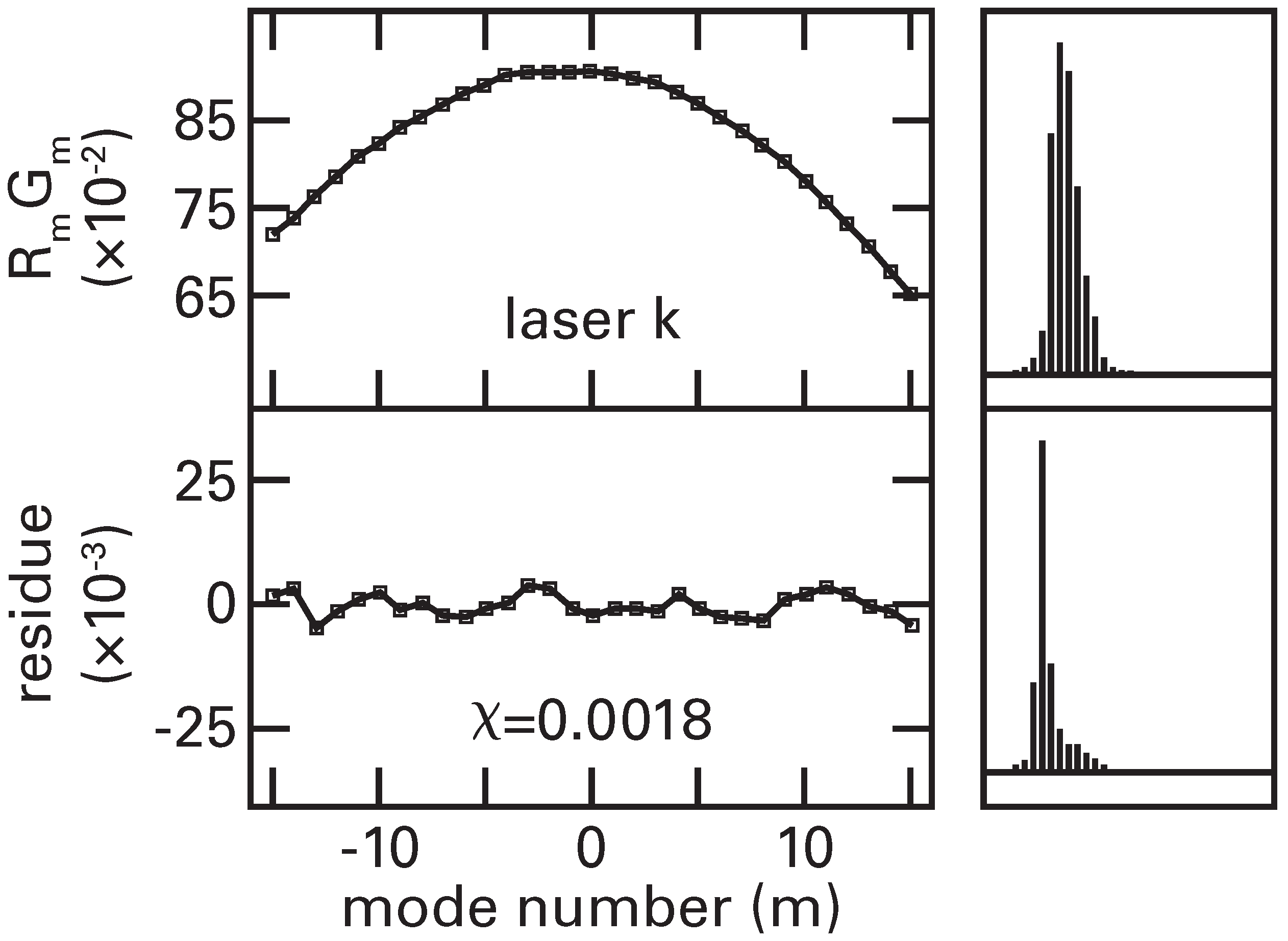
Gain guided lasers had smaller residues in the below-threshold RG product than index guided lasers and also ran more multimode with smoother above-threshold spectral envelopes than index-guided lasers. Figure 11 and Figure 12 show the RG products, the residues, and the extremes of the above-threshold spectral output for two different lasers. A correlation between the residue, and the above-threshold spectral output is clear from the figures.

Hayward also obtained a correlation between scattering centres as measured by $DO{P}_z$ and modulation of the below-threshold spectra of the lasers [38]. He calculated rms residues of the RG product for 16 lasers for which $DO{P}_z$ had been measured, and correlated these residues with the rms scattering parameter as determined by the $DO{P}_z$ measurements.

These two correlations, between the spectral output and the RG residue, and between the scattering as measured by $DO{P}_z$ and the RG residue, support the hypothesis that the spectral output is set by the strength and number of internal scattering centres, and that internal scattering might dominate any effects caused by guiding-enhanced capture of spontaneous emission, population beating, or other nonlinear process. I add that external feedback, whether intentional or unintentional, can also affect greatly the spectral output and along with internal scattering, should be the first or second suspect in understanding the spectral output.

Internal scattering and coherent external feedback alter the RG product and this affects the distribution of power amongst the modes of the laser. Items placed near the laser and in the beam path, such as light collection lenses and rear facet monitors, are usually sources of RG product altering external, coherent feedback.

We were thus able to explain the the steady state spectral properties of diode lasers without reference to a gain-guiding enhanced capture of spontaneous emission, population beating, asymmetric processes, or other non-linear phenomena. The spectral properties could be explained adequately using a simple homogeneously saturated Fabry–Pérot model with resonate enhancement of the RG product owing to internal scattering or wavelength-dependent, coherent external feedback.

J. E. Hayward also performed spectrally resolved measurements on $1.3\mathsf{\mu }$m InGaAsP diode lasers that were operated in a short-external-cavity to force single-mode operation [39]. He found evidence for a symmetric, mode-dependent reduction of gain for powers greater than 5 mW; the power in the lasing mode saturated, the power in the adjacent modes increased, and the total power continued to increase linearly with current. Hayward’s results are consistent with spectral hole burning and suggest, for the devices studied, that the stimulated recombination rate by the lasing mode was competing with the ability of charge-carrier scattering processes to maintain a thermal distribution of carriers in the energy bands of the InGaAsP diode laser.

The observed saturation of the intensity of the lasing mode appears to arise “almost entirely from depletion of the population inversion, rather than from any nonlinearity in the stimulated emission process”, as pointed out by Gordon [5] and quoted in the Introduction of this paper, and that the “saturation depends only upon the time average power”. The gain coefficient was altered to include a symmetric hole and this gain coefficient was used in the expression for the single-pass gain, Equation (8), to model successfully the hole burning [39], (Appendix B of [35]) using the Fabry–Pérot model presented in this paper.

5. Conclusions

This paper reviews, over a limited scope, work on understanding the spectral output of semiconductor diode lasers.

Analytic solutions to a simplified set of coupled, non-linear rate equations that describe the amplification of light for steady-state propagation through a homogeneously broadened amplifier are given. These analytic solutions give the single-pass gain and amplified spontaneous emission in a transcendental form and are used in a Fabry-P erot model for the steady-state spectral output of diode lasers. It is shown that the steady-state spectral output of diode lasers can be explained with this homogeneously-broadened Fabry–Pérot model and that the spectral output depends critically on the reflectance-gain (RG) product and the amount of spontaneous emission that couples into the modes.

The homogeneously-broadened Fabry–Pérot model correctly predicts exponential single-pass gain for low pumping rates and saturation of the single-pass gain near and above threshold. The model appears to include spontaneous emission correctly and thus can explain the dependence of the spectral output on facet reflectance (lasers tend to run more single mode after application of high-reflectance facet coatings and more multi-mode after application of low-reflectance facet coatings) and the differences in the spectral output between gain-guided and index-guided lasers (gain guided lasers tend to operate more multi-mode than index-guided lasers).

The model was used to explain the modulated spectral envelope of diode lasers based on scattering and wavelength-dependent feedback, rather than non-linear effects. The existence of internal scattering centres was experimentally determined from measurements of the degree of polarization of electroluminescence along the active region of specially prepared lasers for above- and below-threshold operation. Parameters that characterized the scattering were measured and used in a homogeneously broadened Fabry–Pérot model to predict the spectral output of the lasers. The measured spectral output agreed with the simulations of the spectral output that used the measured scattering parameters as input.

This simplified or toy model provides an understanding of the role of spontaneous emission and the RG product in the spectral output of diode lasers. The RG product is affected by resonant enhancement of selected modes by unintentional and intentional effects, such as internal scattering and external coherent feedback. Coherent feedback, whether internal to the laser as scattering centres or external to the laser, causes resonant enhancement of selected modes, whereas incoherent feedback increases the amount of spontaneous emission that is coupled into the modes.

Both coherent and incoherent feedback affect the steady-state spectral output of a homogeneously broadened laser. A homogeneously broadened Fabry–Pérot model of a laser appears to incorporate correctly the resonator, single-pass gain, and spontaneous emission, all of which are important in understanding the spectral output of a homogeneously broadened laser. As such, there are strong reasons to recommend the use of a homogeneously broadened Fabry–Pérot model of a laser for understanding operation of a diode laser.

References

- Allen, L.; Eberly, J.H. Optical Resonance and Two-Level Atoms; Dover Publications, Inc.: New York, NY, USA, 1987. [Google Scholar]
- Mukai, T.; Inoue, K.; Saitoh, T. Homogeneous gain saturation in 1.5 μm InGaAsP travelling-wave semiconductor laser amplifiers. Appl. Phys. Lett. 1987, 51, 381–383. [Google Scholar] [CrossRef]
- Kesler, M.P.; Ippen, E.P. Sub-picosecond gain dynamics in GaAlAs laser diodes. Appl. Phys. Lett. 1987, 51, 1765–1767. [Google Scholar] [CrossRef]
- Göbel, E.O.; Hoger, H.; Kuhl, J.; Polland, H.J.; Ploog, K. Homogeneous gain saturation in GaAs/AlGaAs quantum well lasers. Appl. Phys. Lett. 1985, 47, 781–783. [Google Scholar] [CrossRef]
- Gordon, E.I. Optical maser oscillators and noise. Bell Syst. Tech. J. 1964, 43, 507–539. [Google Scholar] [CrossRef]
- Cassidy, D.T. Comparison of rate-equation and Fabry–Pérot approaches to modeling a diode laser. Appl. Opt. 1983, 22, 3321–3326. [Google Scholar] [CrossRef] [PubMed]
- Cassidy, D.T. Analytic description of a homogeneously broadened injection laser. IEEE J. Quantum Electron. 1984, 20, 913–918. [Google Scholar] [CrossRef]
- Cassidy, D.T. Analytic description of a homogeneously broadened injection laser–extension to include a waveguide scattering absorption loss. IEEE J. Quantum Electron. 1984, 20, 1156–1162. [Google Scholar] [CrossRef]
- Cassidy, D.T. Consequences of a lower level population on the modelling of a homogeneously broadened injection laser. Appl. Phys. Lett. 1984, 44, 489–491. [Google Scholar] [CrossRef]
- Cassidy, D.T. Differential quantum efficiency of a homogeneously broadened injection laser. Appl. Opt. 1984, 23, 2870–2873. [Google Scholar] [CrossRef]
- Cassidy, D.T. Spontaneous-emission factor of semiconductor diode-lasers. J. Opt. Soc. Am. B 1991, 8, 747–752. [Google Scholar] [CrossRef]
- Morrison, G.B. Modelling the Spectra of Distributed Feedback Lasers. Ph.D. Thesis, McMaster University, Hamilton, ON, Canada, 2002. Available online: http://hdl.handle.net/11375/6196 (accessed on 19 June 2021).
- Morrison, G.B.; Cassidy, D.T. A probability-amplitude transfer matrix model for distributed-feedback laser structures. IEEE J. Quantum Electron. 2000, 36, 633–640. [Google Scholar] [CrossRef]
- Lamb, W.E., Jr. Anti-photon. Appl. Phys. B 1995, 60, 77–84. [Google Scholar] [CrossRef]
- Hakki, B.W.; Paoli, T.L. Gain spectra in GaAs double-heterostructure injection lasers. J. Appl. Phys. 1975, 46, 1299–1306. [Google Scholar] [CrossRef]
- Marcuse, D. Classical derivation of the laser rate equation. IEEE J. Quantum Electron. 1983, QE-19, 1228–1231. [Google Scholar] [CrossRef]
- Cassidy, D.T. Explanation of the influence on the oscillation spectrum of diode lasers for a change of facet reflectivity. J. Appl. Phys. 1985, 57, 987–989. [Google Scholar] [CrossRef]
- Plumb, R.G.; Curtis, J.P. Channelled substrate narrow stripe GaAs/(GaAl)As lasers with quarter wavelength facet coatings. Electron. Lett. 1980, 16, 706–707. [Google Scholar] [CrossRef]
- Ettenberg, M.; Botez, D.; Gilbert, D.; Connolly, J.; Kowger, H. The effect of facet mirror reflectivity on the spectrum of single-mode CW constricted double-heterojunction diode lasers. IEEE J. Quantum Electron. 1981, 17, 2211–2214. [Google Scholar] [CrossRef]
- Cassidy, D.T. Influence on the steady-state oscillation spectrum of a diode-laser for feedback of light interacting coherently and incoherently with the field established in the laser cavity. Appl. Opt. 1984, 23, 2070–2077. [Google Scholar] [CrossRef] [PubMed]
- Wang, J.; Cassidy, D.T. Investigation of partially coherent interaction in fiber Bragg grating stabilized 980-nm pump modules. IEEE J. Quantum Electron. 2004, 40, 673–681. [Google Scholar] [CrossRef]
- Cassidy, D.T. Technique for measurement of the gain spectra of semiconductor diode lasers. J. Appl. Phys. 1984, 56, 3096–3099. [Google Scholar] [CrossRef]
- Bracewell, R.N. The Fourier Transform and Its Applications, 3rd ed.; McGraw-Hill Companies: New York, NY, USA, 2000. [Google Scholar]
- Wang, H.; Cassidy, D.T. Gain measurements of Fabry–Pérot semiconductor lasers using a nonlinear least-squares fitting method. IEEE J. Quantum Electron. 2005, 41, 532–540. [Google Scholar] [CrossRef]
- Bonnell, L.J.; Cassidy, D.T. Alignment tolerances of short-external-cavity InGaAsP diode lasers for use as tunable single-mode sources. Appl. Opt. 1989, 28, 4622–4628. [Google Scholar] [CrossRef]
- Bonnell, L.J. Single Mode Tunable Short External Cavity Semiconductor Diode Lasers. Master’s Thesis, McMaster University, Hamilton, ON, Canada, 1989. Available online: http://hdl.handle.net.libaccess.lib.mcmaster.ca/11375/25168 (accessed on 19 June 2021).
- Peters, F.H. Spatially and Polarization Resolved Electroluminescence of 1.3 μm InGaAsP Semiconductor Diode Lasers. Ph.D. Thesis, McMaster University, Hamilton, ON, Canada, 1991. Available online: http://hdl.handle.net/11375/8384 (accessed on 19 June 2021).
- Peters, F.H.; Cassidy, D.T. Spatially and polarization resolved electroluminescence of 1.3 μm InGaAsP semiconductor diode lasers. Appl. Opt. 1989, 28, 3744–3750. [Google Scholar] [CrossRef] [PubMed]
- Peters, F.H.; Cassidy, D.T. Effect of scattering on the longitudinal mode spectrum of 1.3 μm InGaAsP semiconductor diode lasers. Appl. Phys. Lett. 1990, 57, 330–332. [Google Scholar] [CrossRef]
- Peters, F.H.; Cassidy, D.T. Model of the spectral output of gain-guided and index-guided semiconductor diode lasers. J. Opt. Soc. Am. B 1991, 8, 99–105. [Google Scholar] [CrossRef]
- Peters, F.H.; Cassidy, D.T. Strain and scattering related spectral output of 1.3-μm InGaAsP semiconductor diode lasers. Appl. Opt. 1991, 30, 1036–1041. [Google Scholar] [CrossRef]
- Peters, F.H.; Cassidy, D.T. Spectral output of 1.3 μm InGaAsP semiconductor diode lasers. IEE Proc. J. Optoelectron. 1991, 138, 195–198. [Google Scholar] [CrossRef]
- Cassidy, D.T.; Peters, F.H. Spontaneous emission, scattering, and the spectral properties of semiconductor diode lasers. IEEE J. Quantum Electron. 1992, 28, 785–791. [Google Scholar] [CrossRef]
- Peters, F.H.; Cassidy, D.T. Scattering, absorption, and anomalous spectral tuning of 1.3 μm semiconductor diode lasers. J. Appl. Phys. 1992, 71, 4140–4144. [Google Scholar] [CrossRef]
- Hayward, J.E. Spectral Properties of 1.3 μm InGaAsP Semiconductor Diode Lasers. Ph.D. Thesis, McMaster University, Hamilton, ON, Canada, 1993. Available online: http://hdl.handle.net/11375/8771 (accessed on 19 June 2021).
- Hayward, J.E.; Cassidy, D.T. Correlation of spectral output and below-threshold gain profile modulation in 1.3 μm semiconductor diode lasers. Appl. Phys. Lett. 1991, 59, 1150–1152. [Google Scholar] [CrossRef]
- Hayward, J.E.; Cassidy, D.T. Experimental confirmation of internal scattering as a dominant mechanism determining the longitudinal mode spectra of 1.3 μm semiconductor diode lasers. J. Opt. Soc. Am. B 1992, 9, 1151–1157. [Google Scholar] [CrossRef]
- Hayward, J.E.; Cassidy, D.T. Correlation between experiments to measure scattering centers in 1.3 μm semiconductor diode lasers. IEEE J. Quantum Electron. 1993, 29, 2173–2177. [Google Scholar] [CrossRef]
- Hayward, J.E.; Cassidy, D.T. Nonlinear gain and the spectral output of short-external-cavity 1.3 μm InGaAsP semiconductor diode lasers. IEEE J. Quantum Electron. 1994, 30, 2043–2050. [Google Scholar] [CrossRef]
Figure 1.
Measured RG product and output power for a GaAs TJS laser. Note the exponential rise and saturation near threshold of the single-pass gain, consistent with the expression for the single pass gain, Equation (8). A better measure of threshold would be to find the intersection of the below-threshold and above-threshold output versus pumping (LI) curves or to find the location of the maximum of the second derivative of the LI curve. The slight difference is not material here. Adapted from Figure 4 of [22], with the permission of AIP publishing.
Figure 2.
Simulated RG product and output power for a GaAs TJS laser. Note the exponential rise and saturation near threshold, consistent with the expression for the single pass gain, Equation (8), and the measured data of Figure 1.
Figure 3.
Experimental data. The lower case letters m, n, o, and p are labels for the four dominant modes shown in this figure and in Figure 4. Adapted from Figure 3 of [7].
Figure 5.
Simulations of the below-threshold spectral output for no short-external-cavity (SXC) in the upper panel and for operation in a SXC in the lower panel. Note the modulated spectral envelope for operation of the laser in an SXC. Above threshold, the SXC laser operated with a SMSR of dB, as shown in Figure 2 of [25]. A measured below-threshold spectral output is shown in Figures 2–4 of [26].
Figure 6.
DOP along the stripe of a laser, showing a strong, discrete scattering centre. Adapted with permission from Figure 4 of [30] ©The Optical Society.
Figure 7.
Measured spectral output of the device shown in Figure 6. Wavelength is along the abscissa and power is along the ordinate. Adapted with permission from Figure 6 of [30] ©The Optical Society.
Figure 8.
Calculated spectral output using parameters obtained from Figure 5. Wavelength is along the abscissa and power is along the ordinate. Adapted with permission from Figure 5 of [30] ©The Optical Society.
Figure 9.
Measured spectral output of a device. Wavelength is along the abscissa and power is along the ordinate. Adapted with permission from Figure 7 of [30] ©The Optical Society.
Figure 10.
Calculated spectral output for a device with a single scattering centre. The strength and location of the scattering centre were chosen from experimental measurements of for the laser. Wavelength is along the abscissa and power is along the ordinate. Adapted with permission from Figure 8 of [30] ©The Optical Society.
Figure 11.
RG product, residue, and worst case above-threshold spectral outputs for a device with a strongly modulated spectral envelope. Adapted with permission from Figure 3 of [37] ©The Optical Society.
Figure 12.
RG product, residue, and worst case above-threshold spectral outputs for a device with a smooth spectral envelope. Adapted with permission from Figure 4 of [37] ©The Optical Society.
Publisher’s Note: MDPI stays neutral with regard to jurisdictional claims in published maps and institutional affiliations. |
© 2021 by the author. Licensee MDPI, Basel, Switzerland. This article is an open access article distributed under the terms and conditions of the Creative Commons Attribution (CC BY) license (https://creativecommons.org/licenses/by/4.0/).
Share and Cite
MDPI and ACS Style
Cassidy, D.T. Spectral Output of Homogeneously Broadened Semiconductor Lasers. Photonics 2021, 8, 340. https://doi.org/10.3390/photonics8080340
AMA Style
Cassidy DT. Spectral Output of Homogeneously Broadened Semiconductor Lasers. Photonics. 2021; 8(8):340. https://doi.org/10.3390/photonics8080340
Chicago/Turabian StyleCassidy, Daniel T. 2021. "Spectral Output of Homogeneously Broadened Semiconductor Lasers" Photonics 8, no. 8: 340. https://doi.org/10.3390/photonics8080340
Note that from the first issue of 2016, this journal uses article numbers instead of page numbers. See further details here.