1. Introduction
The wide range of applications of liquids and determining their properties, especially the temperature changes within the working fluid, play a key role in many sectors of industry and research. Depending on the application, determining such temperature changes can be a crucial step in determining the end-result and efficiency of the process. For this reason, determining temperature changes through non-contact, non-destructive optical methods is very convenient.
Non-contact and non-destructive optical interferometric methods have found a wide range of applications. The discovery of the wave property of light by Thomas Young with its double slit experiment and the interference phenomenon opened up an entire range of possible applications based on the wavefront comparison involving the interference of wavefronts, providing full-field refractive index data to evaluate temperature profile [
1,
2]. Digital holographic interferometry (DHI) stands as one of these methods, and it is considered as belonging to the group of the most accurate methods [
3]. Combining high sensitivity and flexibility, this method is attractive to be used for research. Moreover, the digital acquisition of data allows for data processing and numerical propagation of the wavefield to any plane of interest [
4]. The direct phase retrieval and its differential nature, make digital holographic interferometry an attractive tool for the study of heat transfer phenomena [
5]. It also provides high spatial and temporal resolution and with automation of the recording and reconstruction process, real time visualization is possible [
6,
7].
There is a vast field of applications of DHI and other interference based methods including: entertainment display [
8], imaging heat transfer and mass transfer [
7,
9,
10,
11,
12,
13], research in free convection [
14,
15], visualization of the 3D velocity vector field in turbulent boundary layer [
6], analysis of supersonic jets [
6], biological (living cell imaging) [
6,
16], environmental applications [
6,
17], precision measurements [
8,
18,
19], small displacements [
20], thermomechanical analysis and non-destructive testing [
6], microscopy and high-resolution volume imagery [
21,
22], vibrometry [
23,
24], topography [
25,
26], process monitoring [
7], computerized tomography [
7,
27], and so on.
This paper aims at investigating heat transfer problems. The amplitude of the propagating object wave through the transparent media is not significantly affected, while the phase of an optical wave is [
5]. DHI is sensitive to the optical phase change and thus can be advantageously used for investigation of this kind of problem. However, as the optical phase is integrated along the optical path, the calculation of the quantity under investigation must be performed with regard to the nature of the physical field that we measure. Three categories of physical fields can be considered:
Two-dimensional temperature field (temperature varies only in one direction);
Symmetrical temperature field (temperature is a function of radius only);
Asymmetrical temperature field (general temperature distribution);
Two-dimensional [
5,
10,
28,
29,
30] and purely symmetrical [
31,
32,
33] fields can be measured by one arm interferometer, only the data processing differs for each category.
Examination of asymmetric fields [
34,
35,
36] could not be generally done without the use of cumbersome tomographic approach. The tomographic approach requires a large number of different projections of the measured field. It is either necessary to use many interferometer arms and many digital sensors in the measurement setup to obtain digital holograms for different viewing directions or the problem could be solved having only one digital sensor and a rotating stage. Rotation of the object is applicable only for steady or periodical coherent (self-similar in each cycle) phenomenon. Very often the tomographic approach cannot be realized due to the mentioned physical limits or technical issues as rotating of the object (particularly for heavy system in liquids) or building multiple-arm interferometer might be very challenging. However, in practice, we often encounter quasi-symmetric fields. Pulsatile jets (PJ) with symmetrical openings are a good example. Such a stream of fluid is represented by the time-mean, periodic (symmetrical) and fluctuating random part, of which the periodic part is of the main interest. Moreover, so far, little effort has been made into the pulsatile jets (PJ) study in liquids, which is more challenging than PJ investigation in gases. Some other phenomena in fluids using DHI have been investigated [
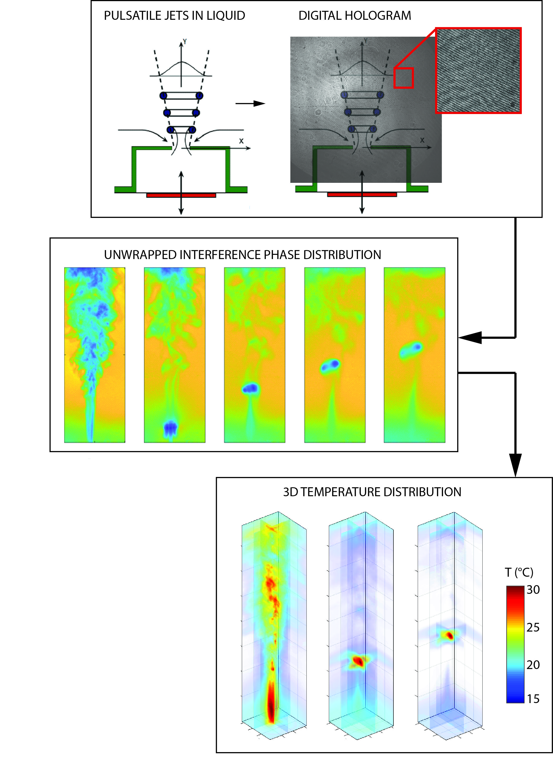
37,
38,
39]. In this paper, we present a single-shot DHI technique suitable for the investigation of quasi-symmetric PJ in fluids, including uncertainty analysis.
2. Pulsatile Jets
In fluid dynamics, a jet is defined as a stream of fluid that is projected through an opening under pressure into a surrounding medium [
40].
When a fluid flows out of the free openings or other outlets into free space, a free jet forms. Based on viscosity, the particles from the surroundings are entrained into the main stream. By absorbing a portion of the jet’s power, the particles play a role in slowing it. With distance, the velocity of the fluid decreases and the jet expands [
41].
A pulsatile jet in the other hand, is a fluid jet generated from fluid oscillations during a periodical fluid exchange between an actuator cavity and surrounding fluid [
42].
Pulsatile jets have a zero-net-mass-flux. This is due to the fact that pulsatile jets suck in the working fluid from the environment and eject it at the end. On the other hand, they allow momentum transfer to the flow. This comes from the asymmetry of the flow conditions across the orifice. By generating vortices in some operational conditions, flow dynamics of the external flow far from the orifice can be affected. Pulsatile jets are inherently pulsatile and periodic, and they can be produced in a number of ways through the use of piezoelectric, electromagnetic (e.g., solenoids), acoustic (e.g., speakers), or mechanical (piston) drivers [
43,
44].
A meaningful advantage of PJs is a relative simplicity of an arrangement: neither blower nor fluid supply piping is required, and only a small electrical power input is needed. This makes jets efficient and attractive [
42,
43,
44].
Applications of pulsatile jets are numerous: improved fluid mixing and higher heat transfer coefficients have been demonstrated in electronic cooling applications using pulsatile jets [
45], applications in flow control in external aerodynamics [
46], in supersonic aircraft [
47], drag reduction improvement in space aircraft [
48], for cooling [
49,
50], etc.
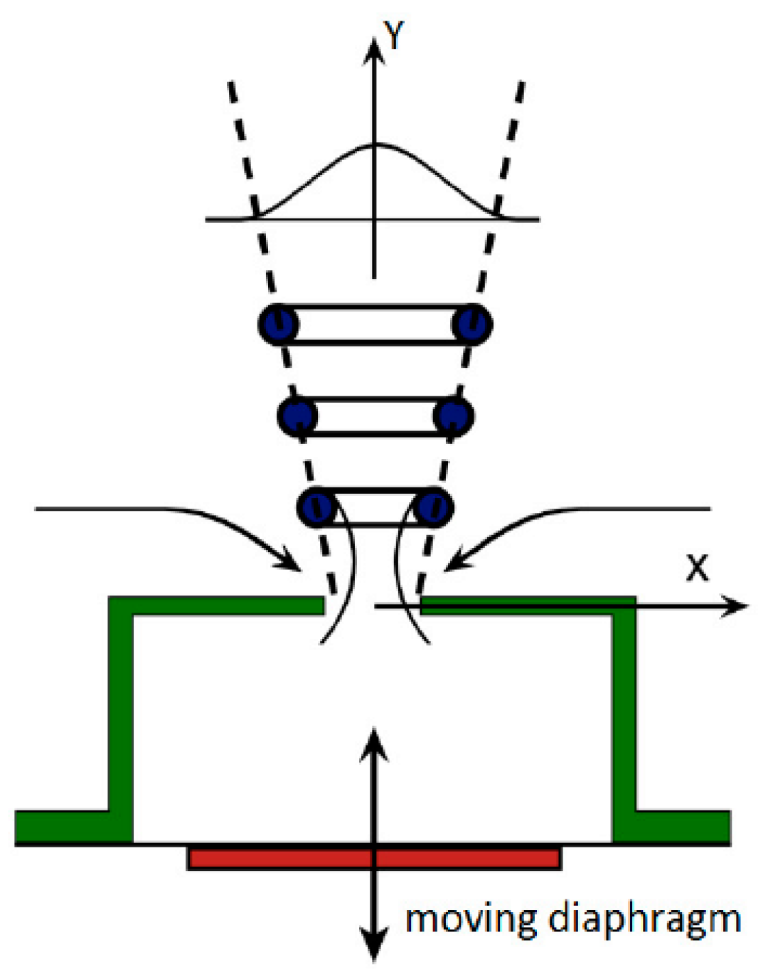
A typical PJ (
Figure 1) actuator consists of a cavity with an oscillating wall (diaphragm or piston). Mechanical energy is transferred from a transducer via oscillating wall to the fluid. The transducer can be arranged either separately from the actuator or it can be integrated into the cavity [
42].
The jet profile after ejections consists of mainly three regions [
52]:
- (I)
The initial region,
- (II)
The transition region,
- (III)
The region of the fully developed jet.
3. Off-Axis Digital Holographic Interferometry
Digital holographic interferometry is a non-contact, non-invasive, whole-field, differential, and highly accurate experimental method for measuring quantities that affect the phase of a light wave passing through or reflected from the measured object [
28,
51].
The hologram is recorded by a camera and the reconstruction is done by numerical methods, by multiplying the digital holograms with the complex amplitude of the reference wave.
In optics, the temperature change is measured via measuring the change of optical properties of the phenomenon under investigation that is caused by such a temperature gradient. Heat and mass transfer problems are specific by the fact that the amplitude of the object wave is not significantly affected while passing through the testing subject, while the phase is very sensitive to such effects. The relative change in the refractive index of the medium that is subjected to thermal gradients with respect to that of the ambient medium have been correlated with the retrieved phase distribution through [
53]:
where
is the change of the refractive index between the actual state and the referential state and
represents the differential distance along the propagation line
. This allows for direct access to the phase. In general, the refractive index distribution can be classified as: flat (refractive index is constant along the optical axis), symmetrical or asymmetrical. For axially symmetric temperature fields, the relation between the refractive index and the phase can be calculated by making use of the Abel transform:
To calculate the temperature, the change of refractive index for temperature must be known. For the case of water,
for
was determined [
53] as:
The link between the temporal change of temperature
(between the moment of measurement and the reference state temperature at
) and the phase change
is given as:
The temperature can finally be computed as:
where
is the ambient fluid temperature at the reference state.
The off-axis spatial intensity interference pattern distribution coming from the interference of the reference and the object wave that hit the camera at any given spatial coordinate
at an angle
introduces spatial carrier frequencies
and
, giving rise to a denser interference pattern which can be mathematically expressed as:
where
represents the reference wave,
the object wave,
represents the additional component (the background intensity),
the multiplicative term (modulation intensity), and
the phase difference between the two arms of the interferometer. Both of the last terms contain the same information, but are conjugate to each other. Therefore, the +1st term should be selected. The interference phase is coded in a cosine modulated fringe pattern. The accuracy with which the quantity of interest can be determined, depends on the phase retrieval method [
15]. By applying the Fourier Transform and making use of its properties, the equation now is:
where
represent the spatial frequency coordinates,
the spatial frequencies that arise from the tilt. The roof symbol
denotes Fourier spectrum. By adjusting the tilt angle between the reference and object wave, both of these three terms can be well separated in the Fourier domain to minimize their overlapping, thus determining the carrier frequencies. The specific order of diffraction can be extracted by means of bandwidth-limited filtering around the specific spatial frequencies. The remaining spectrum
is no longer Hermitean, so the inverse FT applied gives a complex field
with non-vanishing real and imaginary parts.
The carrier frequencies
and
are set in order to correctly separate all spectral components while at the same time respecting the Nyquist sampling criterion through a small tilt in between the object and the reference wave. The maximum angle
between the two interfering waves is expressed as:
while the maximum frequency is limited by the Nyquist frequency
, which is defined by the digital sensor pixel extension
ξ as
.
The spectral bandwidth of reflects the slope of the interference phase : , where denotes the gradient. influences the size of the applied bandpass filter window and optimal value of carrier frequencies. It is important to note that the spectral bandwidth cannot exceed the spatial-frequency bandwidth of the pixelated digital sensor.
The complex field
represents an optical field at a certain initial plane. In the case of lensless DHI, the optical field
is associated to the object plane while for image plane DH (using lens to image the object),
stands for the image plane. Using diffraction theory, one can propagate optical fields from object to image plane (lensless DHI) or focus around the image plane (image plane DHI). Diffraction theory describes the propagation of optical fields and allows for the numerical reconstruction of images which are each described by its intensity and phase. Complex optical fields in the image plane
are calculated using the Sommerfeld formula, which decribes the diffraction of light at distance
from the initial plane. The Sommerfeld integral can be solved by Fresnel approximation which in the discrete finite form is expressed as [
53]:
where
,
and
represents the pixels of the camera, and
is the distance of the phase object from the sensor of the camera. The stored holograms have
discrete values, with pixel distances
and
, with physical size of the recording area of the camera to be
.
represents the conjugated of discrete numerical reference wave, which is used for the reconstruction of the sharp real image at distance
. By digitally reconstructing the diffracted field, we have direct access to the amplitude image and the phase image [
6]:
The phase of the field is calculated using the arctangent function, and consequently, the result will be contained within the interval [−π, +π], i.e., modulo 2π. In the case of image plane DHI, when the image is formed directly on the digital sensor, in (10) can be replaced directly by the complex field
The phase
is affected by any aberrations of the optical system and thus it is usually not of the main concern. In DHI, firstly a digital hologram for the reference state (i.e., no phenomenon) is captured and processed as aforementioned in order to retrieve the phase denoted as
. In further steps, digital holograms during a phenomenon under investigation occurrence are captured and processed leading to phase fields
. The interference phase
showing only the measured phenomenon can then be determined in a pointwise manner by a modulo of
substraction [
53]:
The estimation of the optical phase of the reconstructed field is key to a large number of applications in digital holography [
6]. The possibility of direct access to the phase difference information is one of the major advantages of digital holographic interferometry [
5].
Tomographic Reconstruction
Tomography is generally a non-invasive imaging technique. It allows for visualization of internal structures without the superposition of over- and under-lying structures [
29]. As said previously, the refractive index distribution can be generally classified into three groups in regard of its distribution: flat, symmetrical, and asymmetrical. The first two represent the simplest case and the easiest to reconstruct the temperature fields.
Tomography in general involves two steps: the recording of the projection data and the reconstruction of the original data that was projected. Projections from many angles in order to be able to faithfully reconstruct the real temperature field are required. The more projections there are, the more exact and reliable the reconstruction will be. This undoubtfully makes the setup more complex and the need of a superfast camera is a must. The recording is done by digital cameras and the captured images represent the projection of the 3D object into 2D images. Although for the case of periodically self-similar repetitive phenomena, only one superfast camera can be used, by changing the angle of recording for each period of the phenomena (by a rotating stage) and synchronizing the recording with the period of repetition. Noise and errors are suppressed by averaging the images with the same phase in different periods.
For axi-symmetrical cases, the procedure is simplified. The tomographic approach makes use of the Abel Transform. The representation of the data obtained by Abel Transform as a function of the angle of projection is called a sinogram. It contains the data from the projection for different angles stored as columns. By applying a filter to suppress some range of oversampled low frequencies in the Fourier domain and a window in order to prevent possible numerical Fourier Transform issues, we obtain what is known as the inverse Abel Transform with filtered back-projection:
where
represents a filter and a window. It expresses the filtered back-projected image for all angles, which are smeared out in space. The filtered back-projection is an analytical method that propagates the sinograms into space for all angles along specific projection paths in order to reconstruct the 3D profile.
4. Materials and Methods
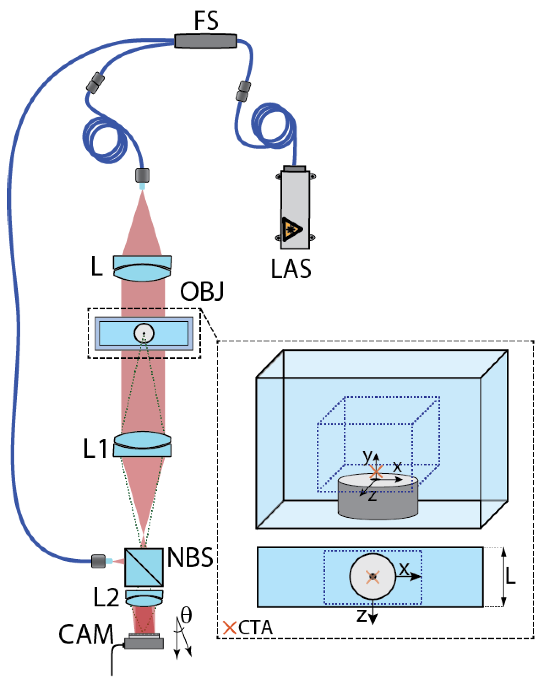
Figure 2 shows a schematic of the holographic setup that was implemented for this study. The setup consists of two portable parts, made for easier transportation and a more compact setup. It is based on the Mach-Zehnder interferometer, which gives as output the interference pattern that is dependent on the refractive index change occurring in the phase object (OBJ). A Mach-Zehnder interferometer consists of two interferometric arms, the object arm and the reference arm. After passing through a fibre-beamsplitter (FS), the laser beam is split into two. The first beam acts as the object wave that passes through the phase object under investigation, while the other beam acts as the reference wave. The object beam is collimated into a parallel beam by a collimator (L) before passing through the water tank containing the pulsatile jet. Before impinging the camera, the object wave passes through lenses L1 and L2, which act as a 0.12× beam expander in order to reduce the beam diameter to fit the digital sensor size. Both waves are recombined and superimposed by a non-polarizing beamsplitter (NBS), collimated by a lens (L2) and redirected to the digital camera (CAM) where the microinterference pattern is electronically recorded for further processing. The reference wave was aligned with the object wave by positioning of the fiber output aiming to NBS. The angle between both waves was set by analyzing the Fourier spectrum in real time. The adjustment of both waves intensities has been made for the highest fringe contrast value possible. A highly coherent helium-neon laser (LAS) of wavelength
with maximal output optical power of 50 mW has been employed for this study. Since holographic interferometry is very sensitive, the optical setup has been put on a vibration-isolated optical table.
The used camera is a UI-3370CP Rev. 2, pixel, pixel size CMOS camera.
The field of view of the measured area was mm2.
The object under study is a pulsatile jet (PJ) with a circular opening of , submerged in a water tank containing water at temperature of . The pulsatile jet is fed with prewarmed water, the temperature of which was predetermined to be around . The warm water passes through the orifice to create the jet profile. Time period of the PJ is , i.e., long enough for the flow to get steady. The PJ period therefore consists of the initial transient stage, steady stage, and final transient stage. The long period phenomenon with a steady flow was chosen on purpose in order to separate random and steady component of the PJ. The inner dimensions of the glass water tank are with wall thickness of and has been filled with water up to the height of .
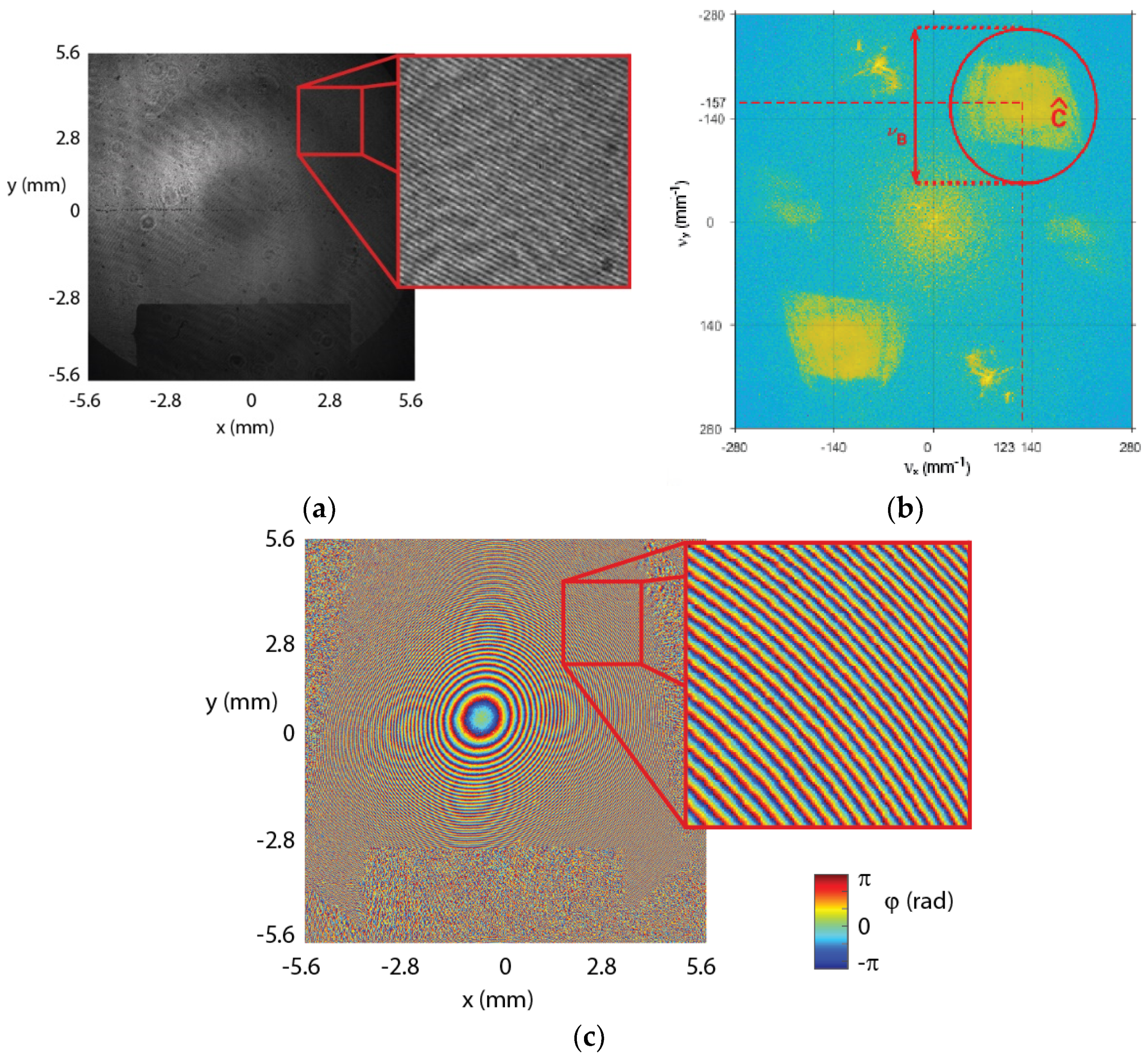
In the first step, all holograms have been recorded and reconstructed by the Equation (9). In total, 314 holograms have been recorded, with some being captured when the system was off and later used as the reference. Example of a hologram is shown in
Figure 3. They have been captured with framerate of
and sampling time of
.
Figure 3b shows the Fourier domain of the reference hologram. Here, the term
can clearly be seen separated from the terms
and
due to the tilt between the reference wave and the object wave, from which the carrier frequencies
and
were introduced by real time observation of the Fourier spectrum while adjusting the reference arm of the interferometer. In order to avoid phase errors from diffraction effects, the angle has been selected to be slightly greater. The choice of the carrier frequencies depends on various factors, as the Nyquist criteria, distance from the detector and its size, and importantly the gradient of phase
. The gradient of phase
, i.e., object wavefront curvature, is high due to the “lensing” effect of the water tank. The digital sensor’s spatial-frequency bandwidth was sufficient in order to cover the spectral bandwidth
of
and the spatial carrier frequencies were adjusted in order to avoid overlapping in the Fourier spectrum. The carrier frequencies were determined to be
and
. This allows for the determination of the tilt angle between both waves with respect to the direction of propagation
to be
and
. A 2D Hanning window with a bandwidth of
and centers
,
,corresponding to the carrier frequencies that have been applied in order to filter the term out, was used in order to retrieve the complex field in Equation (7).
The same procedure is applied to all digital holograms. It is important to note that the filtering window remains unchanged for all holograms. The interference phase between a hologram captured at time t with respect of the reference hologram has been calculated as modulo of
(11). The wrapped interference phase distributions were free of undersampled areas and therefore has been successfully unwrapped through the Goldstein algorithm [
54]. The process of unwrapping introduces itself error uncertainty. Mostly, these uncertainties are too small to be taken in consideration. Phase aberrations are present, apart from the dynamic phase change from the measured phenomena, in both the reference and the object beam along the whole optical path. Phase aberrations can come from different contributors, such as the improper selection of carrier frequencies, tilt between the reference and object wave, imperfections in the optical components or the misalignment of the optomechanical components of the interferometers. The filled water tank in steady state introduces significant wavefront error.
Figure 3c illustrates the phase aberration from the combined wavefront hitting the sensor of the camera. Since these aberrations are stationary (time invariant) and come from the optical system, in case of digital holographic interferometry where the phase fields are compared to the reference state that carries the same phase field aberration, these aberrations vanish from calculation. This is one advantage of this technique, since all imperfections in the optomechanical elements become less relevant and carrier frequencies do not have to be precisely set. Therefore, the state reference has been captured shortly before the exhibition of the phenomena of interest.
Since we deal with the case of symmetrical orifice, we assume the development of a symmetric temperature field. Based on this assumption, only capturing one projection for the analysis is supposed to be sufficient in order to retrieve the refractive index field in Equation (2).
The temperature field has been retrieved by using the inverse Abel Transform. This was done by taking one row of the phase data and reconstructing the slice. The reconstruction of the 2D plan sliced has been done by the filtered back-projection method, which later were all stacked on top of each other to form the 3D temperature profile.
In real experiment, steady (symmetrical) and random components of the flow occur. Within the middle stage of the PJ period when the PJ flow is laminar, we separated the steady (symmetrical) and random flow components using averaging of phase maps at different time instants. This reveals how valid the assumption about the symmetrical flow is.
5. Results
The results from the interferometry-based visualization of temperature fields from a jet with warm water have been discussed here. Some of the illustrated results are restricted only to the relevant regions for study and are a projection of the testing subject, hence they are predominantly two-dimensional and averaged along the optical path. Three dimensional reconstructions are also presented.
Temperature values measured through off-axis digital holographic interferometry are relative, meaning that a starting point must be a priori known. The temperature of the water in the tank has been measured right before the experiment started with a thermometer and is assumed to be only slowly varying at the edge of the digital camera field of view. The temperature has been computed using Equation (5).
Phase and temperature values are displayed according to the color bar legends located on the side of the results. In the case of 2D visualization, displayed values must be understood as averaged values along the optical propagation path.
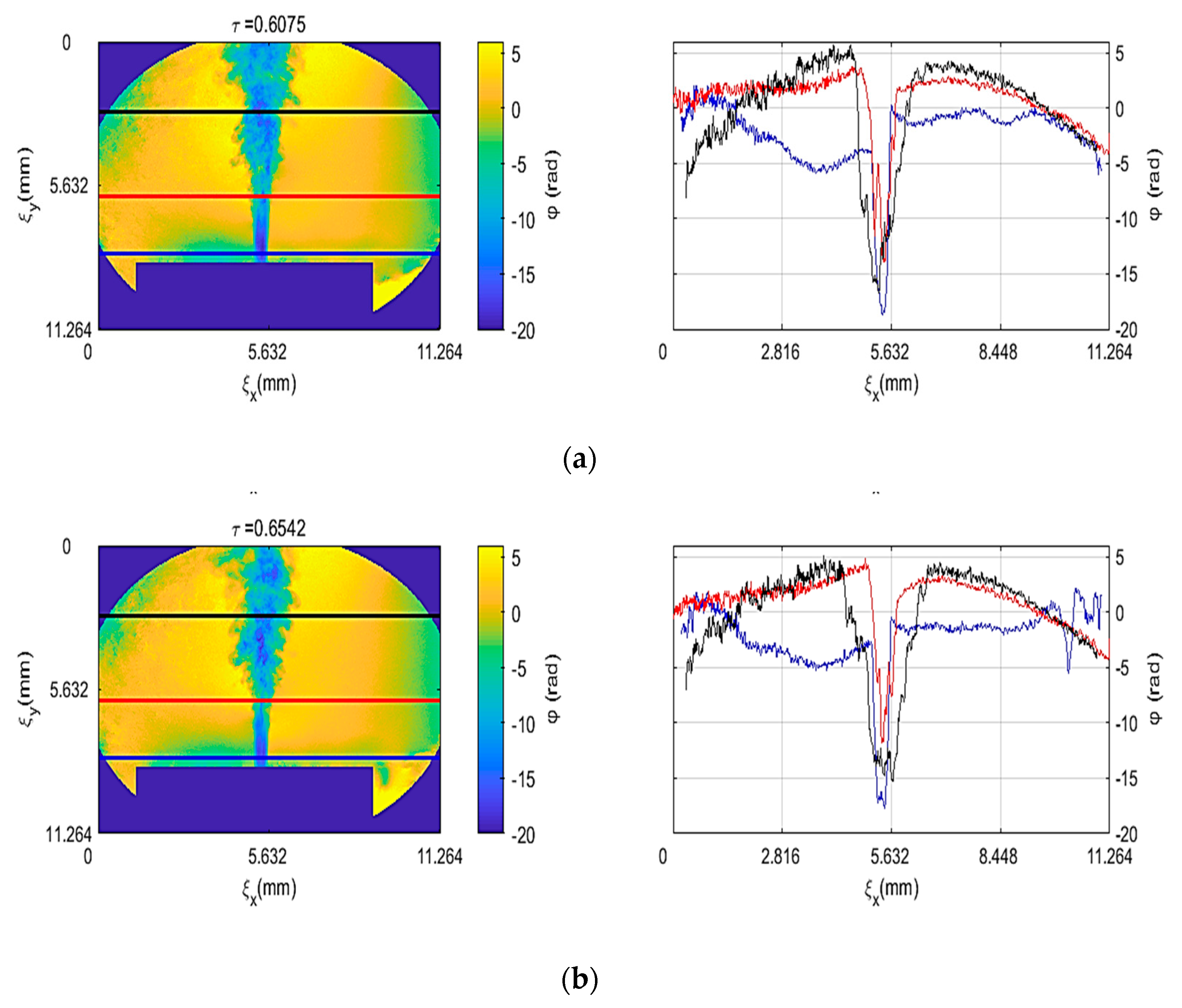
Figure 4 shows the symmetrical whole-field interference phase profile of warm water flowing out from a single circular orifice with a diameter of
m from the orifice at two different instants of time. Three cross sections were drawn for analysis. It shows the effect of temperature on the refractive index of water at the three cross sections, which are plotted in the graphs right next to them. As expected, the phase is lower at the vicinity of the orifice where the warm water comes out and the phase change is less at the distance where the warm water mixes with the colder water. The time instants were chosen when the jet profile was the most stable.
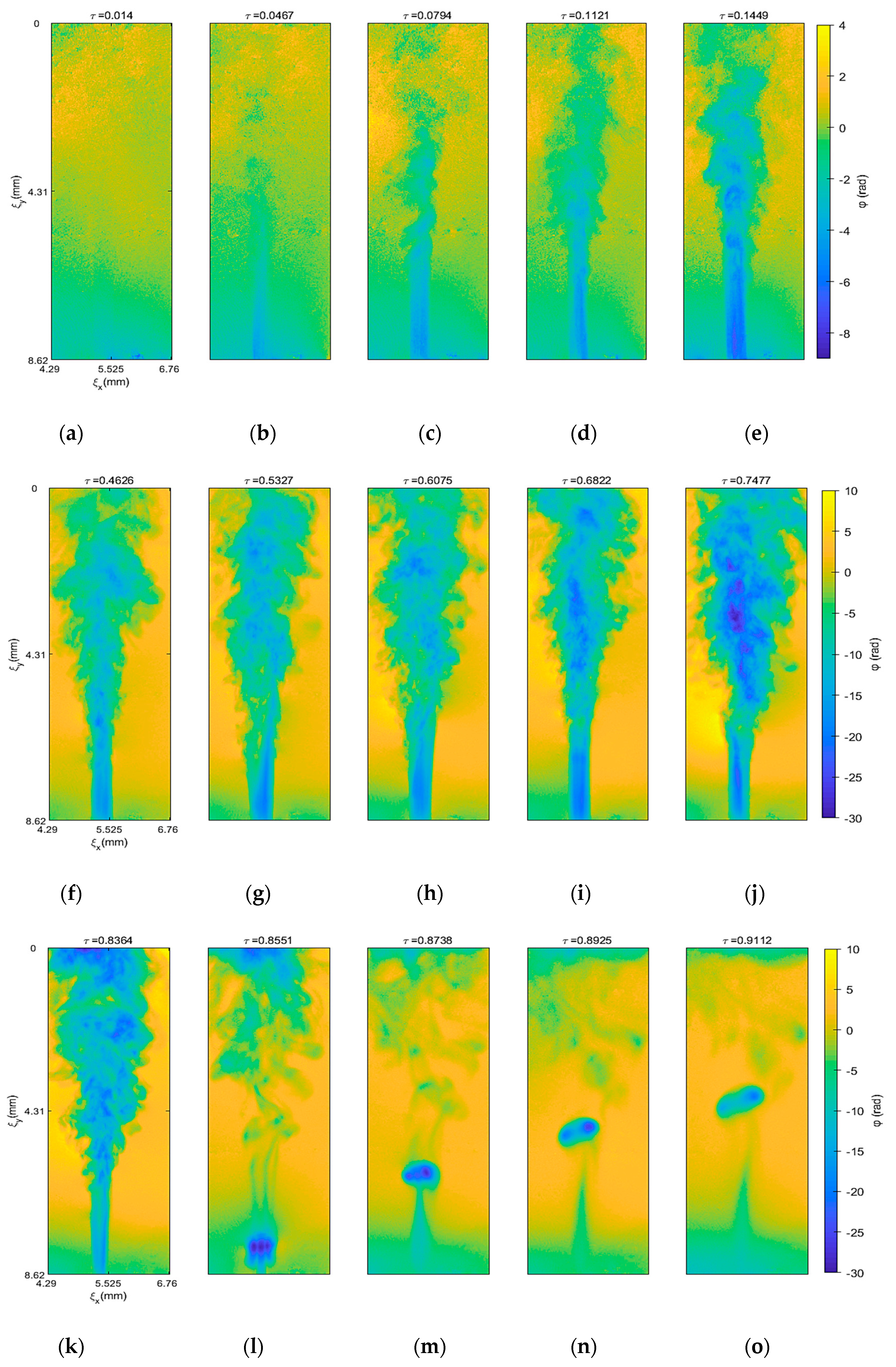
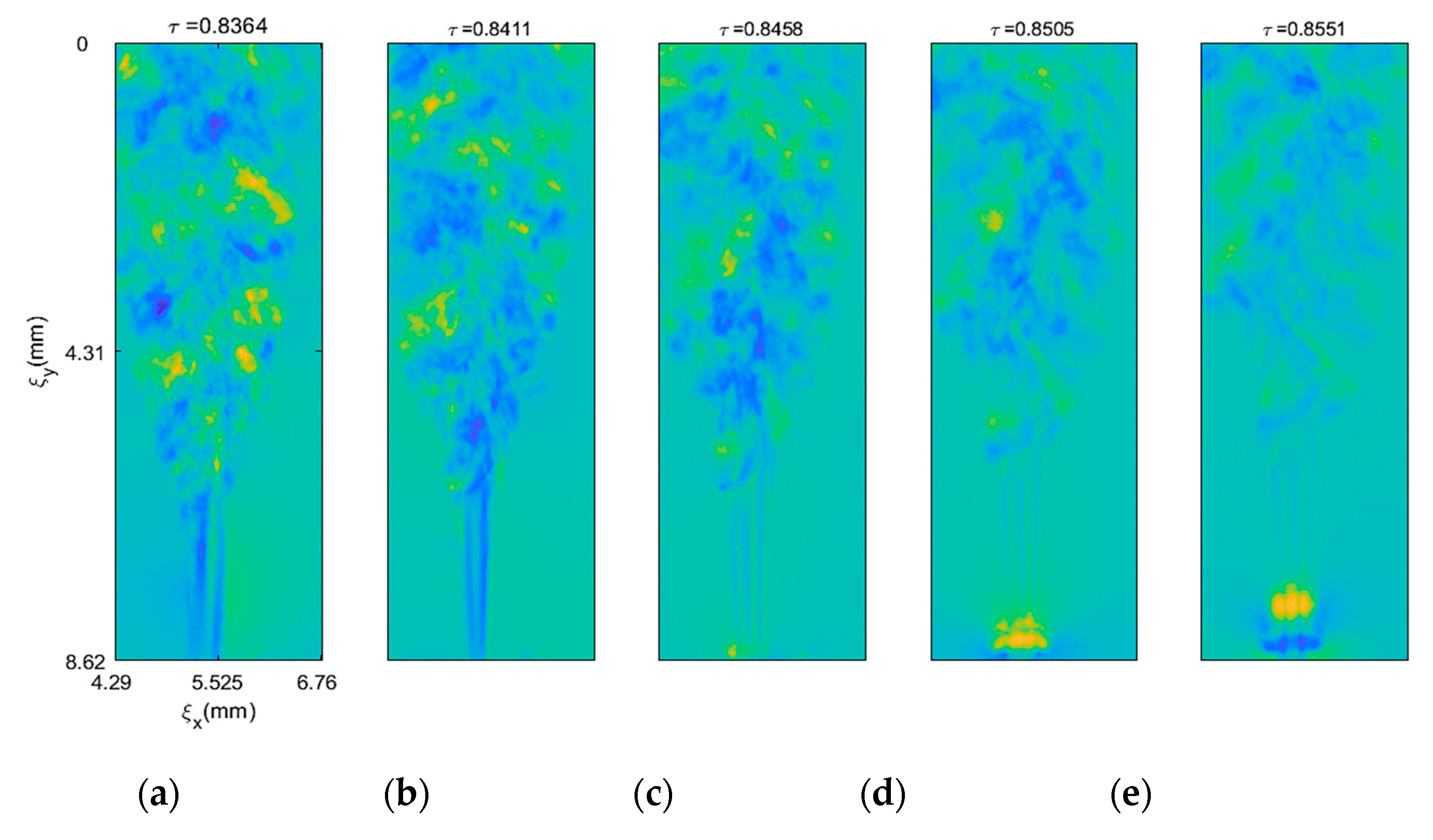
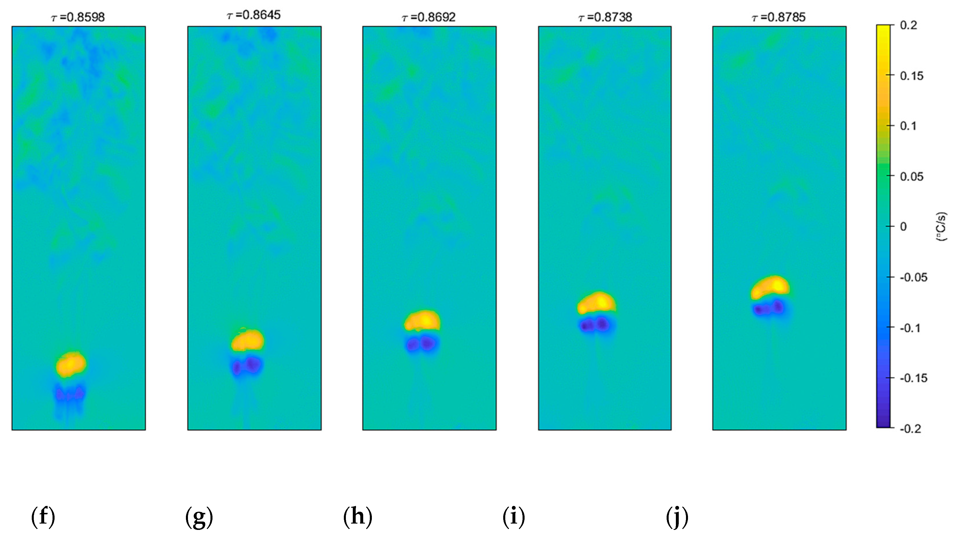
Figure 5 shows the time development of the phase profile of the jet stream coming out of the orifice. Several points in time have been selected to show the formation of the characteristic jet profile and its development in time. The first row shows the beginning when warm water starts flowing under pressure. The jet profile can be seen clearly established on the second row. On the last row, after stopping the incoming warmer water, a small pocket of warm water can be seen moving upwards. Digital holographic interferometry can clearly visualize the PJ position and evolution and track its movement in space and time. Retrieved phase distributions and characteristics of PJs deduced from them are valid regardless of the kind of measured phenomenon. However, in order to quantitatively retrieve refractive index distribution and hence temperature field distribution, the phase fields are assumed to be symmetrical. This assumption introduces some uncertainty, as discussed further in the text.
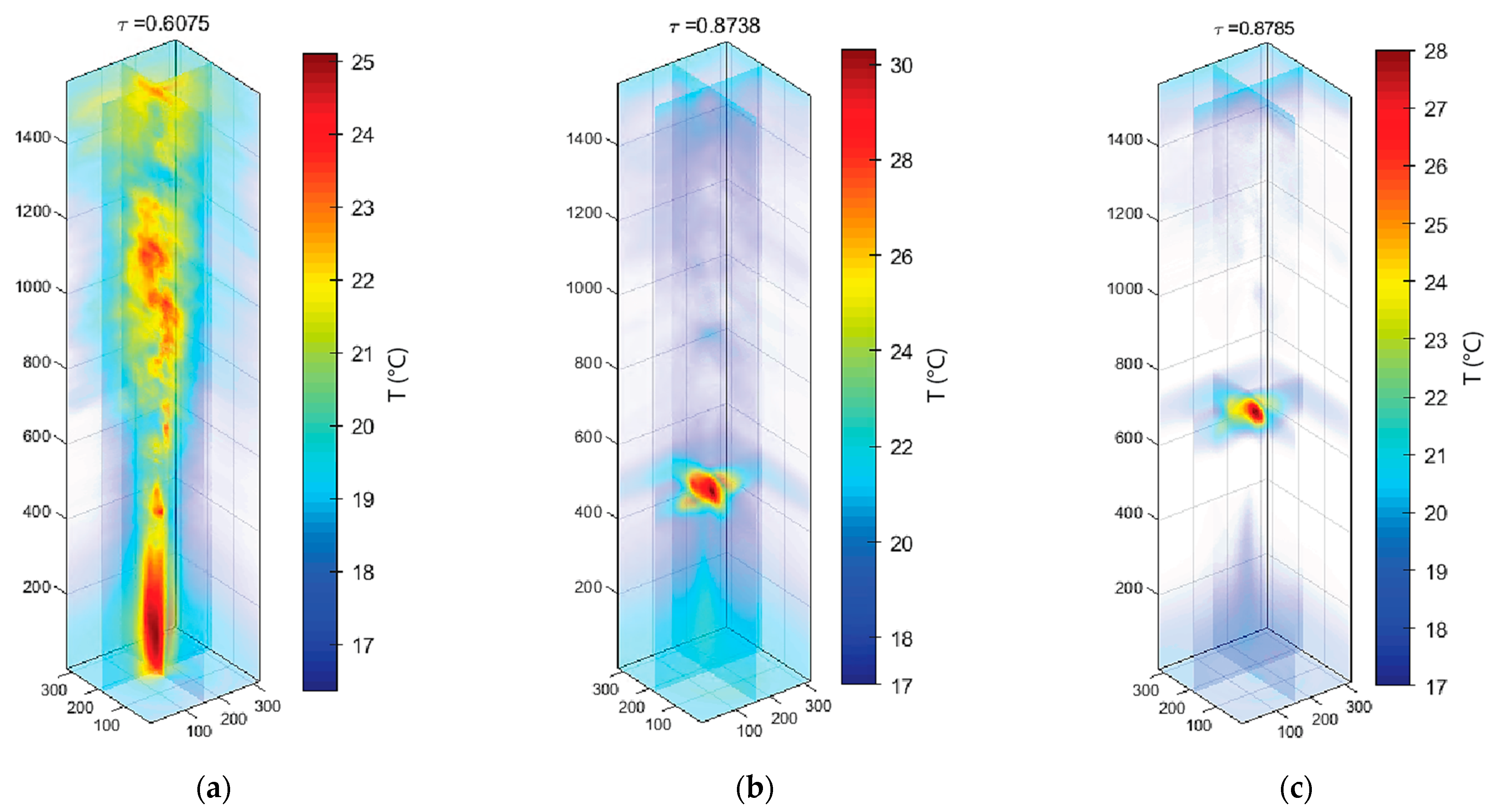
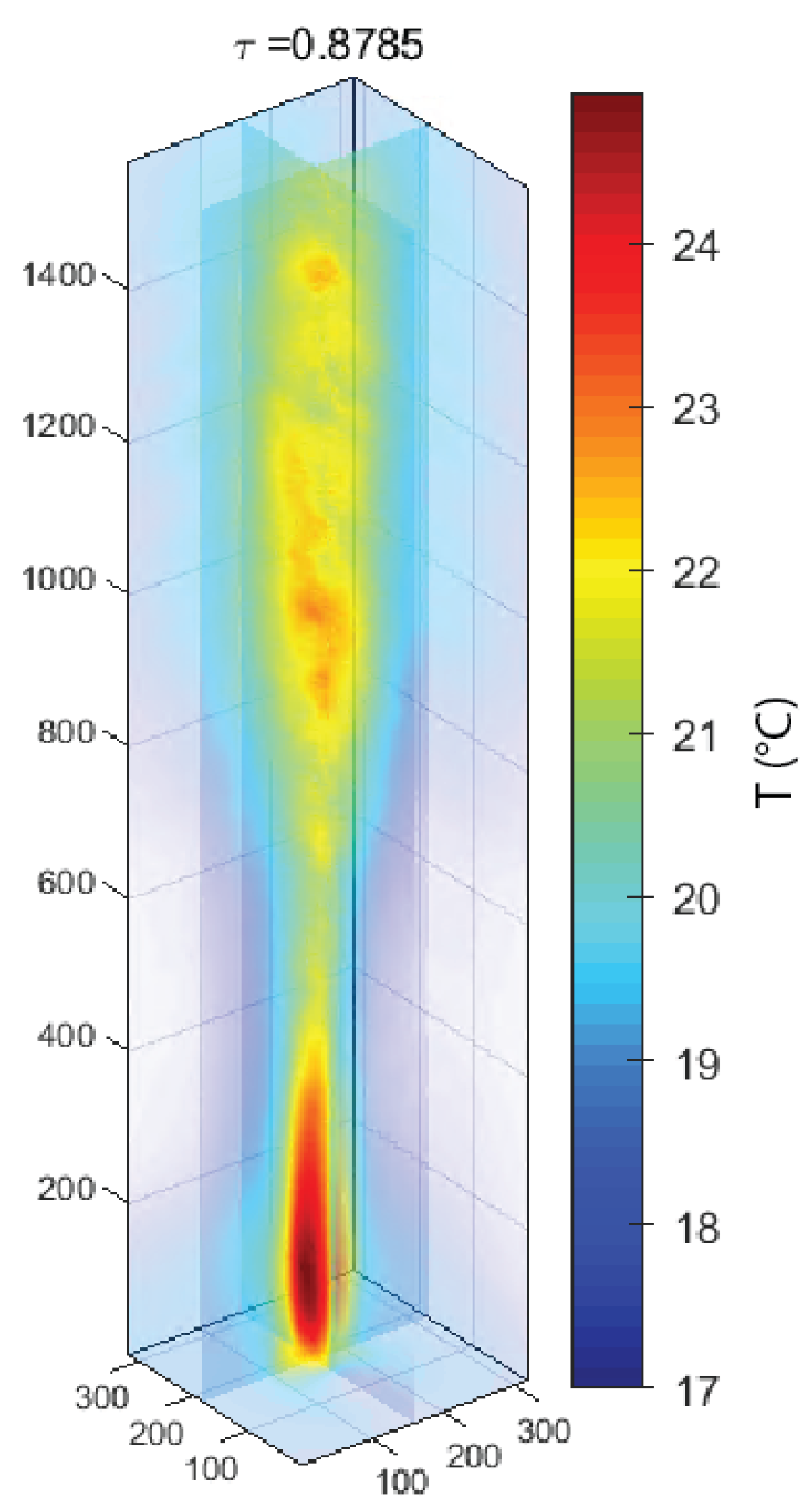
Figure 6 shows the 3D reconstruction using inverse Abel transform of the jet profile at three different instants in time. The first one depicts the 3D reconstruction of the jet profile, while the two consecutive ones depict the reconstruction of the small warm water pocket. Tracking can be done from frame to frame.
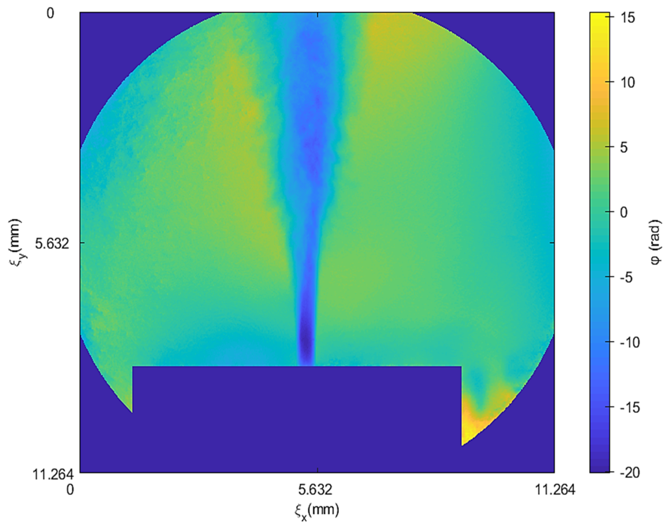
However, the condition on symmetry is not fully met. The averaging of many phase fields during the steady flow stage, results in the suppression of the signal fluctuation (random) component. The averaged phase profile over 15 consecutive frames is shown in
Figure 7. The averaging time is
and thus faster random components are suppressed.
Figure 8 shows the tomographic reconstruction from the averaged phase values (see
Figure 6a for comparison).
In order to observe the thermal phenomena happening in the liquid in more detail, the dynamic range of the temperature values must be reduced. Therefore, temporal finite difference temperature
is computed. It has been computed as:
Fluid mixing can be seen on the first row of images of
Figure 9. Where colder water from the tank is shown in blue color being pulled and mixed with warmer water, shown with yellowish color. The second row depicts the small warm water pocket traveling upward once the flow through the circular orifice was stopped. As seen, if the speed of the camera is high enough, this technique allows for its tracking.
Limits and Errors of Interferometry in Liquids
Several sources of error that are influencing our measurement are considered. Fundamentally, DHI measures interference phase , which is further converted into refractive index variation and in the last step the temperature change is determined, assuming . Each of these steps suffer from some uncertainties.
The uncertainty of interference phase measurement comes from factors such as misalignment and settling of optical components, fluctuation of laser wavelength, electronic noise, and external unstable environment conditions [
15]. The phase noise for our measurement is estimated to be
. The value was determined from experimental data (without the phenomenon) as the peak-to-valley value of an unwrapped phase map after low order polynomial subtraction (i.e., high spatial frequency components were considered as the noise). Such phase error contributes to temperature measurement uncertainty
. However, the major uncertainty source is in the second step, i.e., the refractive index distribution calculation using inverse Abel transform.
We assumed weakly-varying refractive index with the approximation of straight rays. Analysis [
55,
56] revealed that even if a diffraction of light is considered, the refractive index uncertainty is always about one order lower than the measured variation of refractive index. However, this is valid for purely symmetrical fields or asymmetrical fields using many projections. Hence, the major source of uncertainty in our case is the assumption of symmetrical field even though the physical field evinces some random fluctuations. In order to estimate validity of the assumption, standard deviation of phase fields during the steady stage of the PJ was calculated as:
where
is the averaged phase, and
is the number of phase maps.
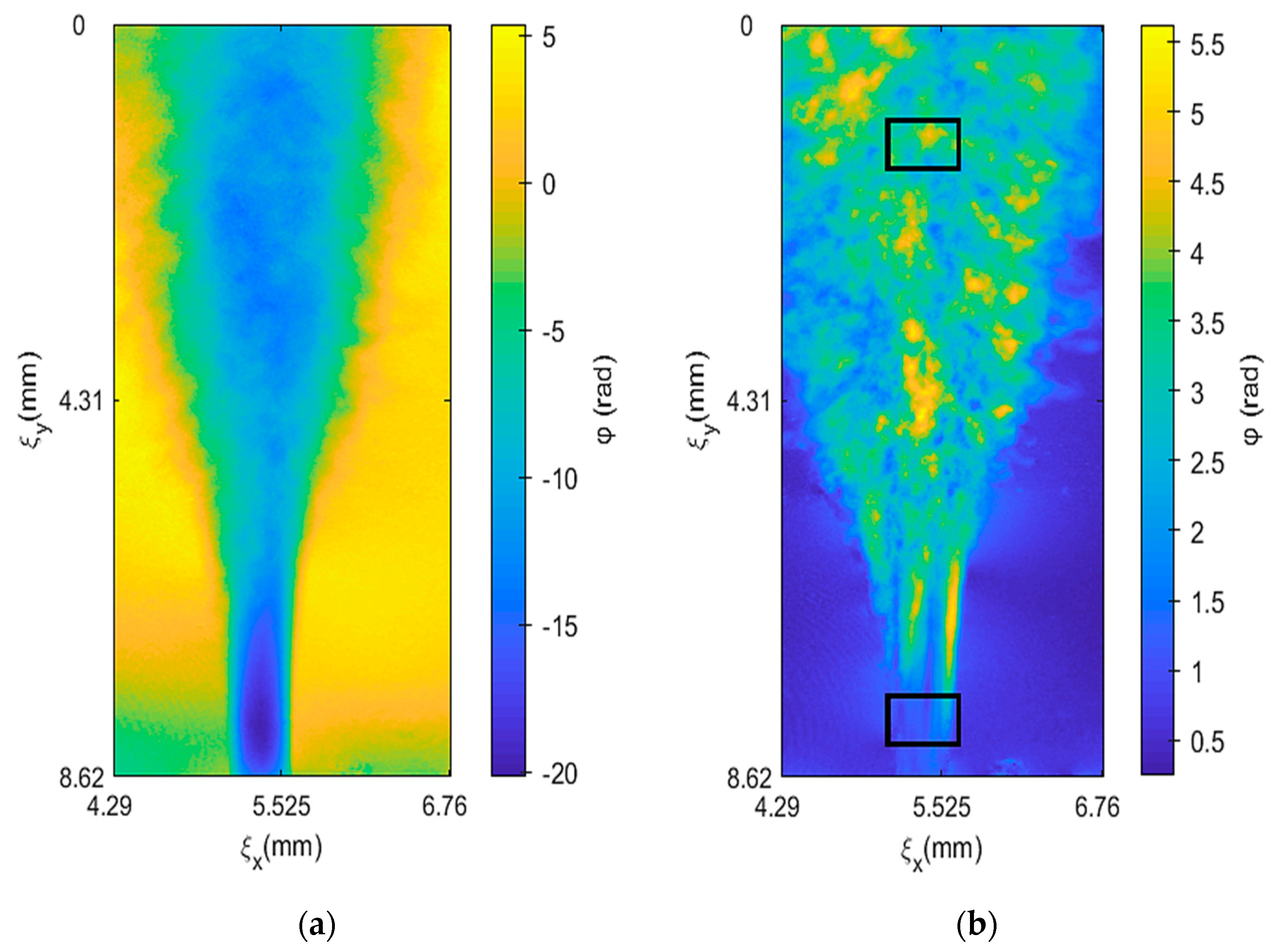
The standard deviation map of interference phase maps has been calculated and shown in
Figure 10, where (a) shows the averaged phase map and (b) shows the standard deviation map. Two regions for evaluation have been selected: one further away in the developed area where the random flow fluctuations are more obvious and one near the opening where almost laminar flow is predicted. The estimated error in the region of the developed puff is
while in the region near the orifice the standard deviation is
.
From
Figure 10 it follows that the assumption on symmetry is the main uncertainty source (one order higher than the aforementioned sources). Assuming flat (2D) field for simplification, the temperature uncertainty can be estimated as
, where
is the orifice diameter. The uncertainty
near the PJ opening is 0.03 °C, which is relatively below 5%. On the other hand, further from the opening, where the random fluctuations play a more significant role
, it is relatively about 15%.
In case of steady flow, averaging of phase maps can filter out the random fluctuations and hence decrease the uncertainty. On the other hand, many phenomena are rapidly time varying, averaging cannot be applied, and the uncertainty ranges are deduced in the range 5–20%.
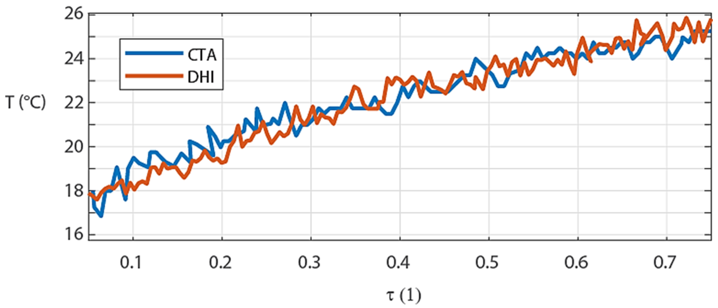
To verify the reliability of DHI we compared the results to results of well-established CTA (Constant Temperature Anemometry). CTA is single point method and therefore we chose one representative point within the measured area that was located on the axis of the orifice approximately 2 mm above the opening. Location of the CTA sensor is illustrated as a red cross in
Figure 2. DHI is a full-field method and therefore we had to pick voxels of the measured temperature distribution corresponding to those values measured by CTA. Results showing a good agreement are plotted in
Figure 11. The red color stands for DHI while blue represents values obtained by CTA. A significant source of the discrepancies in results between DHI and CTA is the fact that both measurements DHI and CTA had to be performed separately at different time due to invasive feature of CTA. Although the initial experimental parameters were set as similar as possible, the environmental conditions as well as behavior of the phenomenon itself could slightly vary between both measurements.
6. Conclusions
A digital holographic interferometric methodology for the measurement of temperature fields through the analysis of the refractive index variation has been implemented. Real-time dynamic temperature field change and visualization of volumetric temperature fields generated by a heated fluid from a pulsatile jet in a water tank through off-axis digital holographic interferometry have been reported. This paper, through the conducted experiment and results, presents and puts off-axis Digital Holographic Interferometry as a powerful technique to visualize symmetrical temperature fields in water created by a periodic pulsatile jet.
The pulsatile jet generator was placed in a water tank filled with water at room temperature. A pulsatile jet with higher temperature was coming out of the orifice with a circular diameter of . A portable Mach-Zehnder interferometer has been used in order to record the holograms with a digital camera. Digital holograms have been evaluated and symmetrical temperature fields have been retrieved using inverse Abel transform.
The main source of uncertainty was the assumption of a symmetric field, although the flow shows turbulence and other asymmetries. Due to the steady flow behavior during the middle part of the period, we estimated that the relative uncertainty of the temperature field measurement near the orifice is below 5%. On the other hand, further from the orifice, where random fluctuations play a more significant role, the relative uncertainty increases up to 15%. This must be considered when using single-shot DHI for symmetrical pulsatile jets investigation.
Results obtained through this study demonstrate a successful appliance of this approach for temperature field measurement in pulsatile jets with water as the working fluid. Our study indicates that digital holographic interferometry can be used to visualize temperature fields, study flows and evaluate their characteristic quantities, and is superior to other conventional methods since it is a non-invasive whole-field technique that can be automated and deliver real time results with high temporal and spatial resolution.


