Article

Wavefront Modulation and Beam Shaping into Arbitrary Three-Dimensional Intensity Distributions

by
Tatiana Latychevskaia
1,2
1
Physics Institute, University of Zurich, Winterthurerstrasse 190, 8057 Zurich, Switzerland
2
Paul Scherrer Institute, Forschungsstrasse 111, 5232 Villigen, Switzerland
Photonics 2021, 8(6), 179; https://doi.org/10.3390/photonics8060179
Submission received: 18 April 2021 / Revised: 18 May 2021 / Accepted: 19 May 2021 / Published: 23 May 2021
(This article belongs to the Special Issue Holography)

Abstract

:
In this study the methods of three-dimensional (3D) wavefront intensity modulation by employing contrast-inverted holography, previously introduced as Gabor inverted holography, are further investigated. The present study provides the recipes for creating 3D wavefront intensity modulations using phase-only and amplitude-only modulators and compares the results. The 3D wavefront modulation using spherical waves is also demonstrated, and the miniaturization of 3D intensity beams is discussed; it is shown that both the resolution and the size of the created 3D structures are ultimately given by the wavelength of the employed radiation. The manuscript also addresses the quality of the formed 3D intensity curves and determines the parameters that provide the best smooth appearance of the 3D curves. The presented methods of 3D intensity wavefront modulation can be realized for all kinds of waves: light, X-ray, electron, etc, provided the modulator can be manufactured for the corresponding wavelength. The methods of 3D intensity wavefront modulation can be applied in various techniques: lithography, micro-robotics, particle trapping, etc.

1. Introduction

Wavefront modulation techniques utilize optical schemes, where an optical element (modulator) transforms the distribution of a passing wave into a pre-defined wavefront distribution at some distance behind the optical element. The distribution of the modulator can be obtained via numerical simulation and then realized as a physical mask or it can be loaded onto a spatial light modulator, as, for example, in the case of light waves. An example of wavefront modulation is focusing X-ray beam into a spot by using a modulator in the form of a Fresnel zone plate. Holography [1,2] is a technique that is widely employed for wavefront modulation, in particular by using so-called computer-generated holograms (CGH) [3,4]. Conventionally, modulators are described by either phase- [5,6] or amplitude-only distributions [7,8,9]. For two-dimensional (2D) wavefront modulation, a modulator’s distribution can be calculated by applying an iterative phase retrieval algorithm, originally proposed by Gerchberg and Saxton [10] as follows. A wavefront is propagated back and forth between the two planes: the modulator and the image plane, and at each plane, a constraint is applied. In the modulator plane, the wavefront must be a phase- or amplitude-only distribution depending on the modulator type. In the image plane, the wavefront must exhibit the pre-designed 2D distribution. A modulator distribution found by an iterative approach [11] allows wavefront modulation into a pre-designed 2D distribution in one plane.
Generating a three-dimensional (3D) wavefront modulation is a somewhat more challenging task. Although holography allows 3D wavefront modulation in the form of a reconstructed 3D object distribution, it does not provide a straightforward approach for creating arbitrary 3D intensity beams, and it is not employed to create such intensity modulations. Only the limited class of 3D curves that are described by analytical functions can be realized as 3D intensity modulation using an analytical function distribution as modulator distribution, for example, Airy beams [8,12,13,14,15], solenoid beams [16] or tractor beams [17]. Attempts to create arbitrary 3D intensity beams were previously made: “Snake beams” were proposed to shape intensity into a curvy beam [18], however the resulting beam wasre made of finite-sized line segments formed in the focal plane of a lens and, therefore, did not create a smooth and arbitrarily distributed 3D intensity beam. A general method for creating truly arbitrary 3D intensity beams, named as “inverted Gabor holography” was recently proposed [7,19]. The inverted holography is different from conventional CHG or other wavefront modulations methods in two ways: (1) Unlike most CGH methods, inverted holography allows 3D (not 2D) shaping of the wavefront; (2) Unlike methods for creating Airy beams, inverted holography can shape the intensity into arbitrary distributed and z-extended 3D intensity beams. The inverted holography was demonstrated as creating unusual and not analytical curves: bending light beams (similar to Airy beams), a beam that splits into two parallel beams, or even a beam with a local “gap” of a zero intensity [7]. Recently, inverted holography was demonstrated for the modulation of electron waves [9].
In this study, the method of 3D wavefront intensity modulation by employing contrast-inverted holography, previously introduced in references [7,19], is further investigated in more detail. In the following sections the principle of 3D wavefront intensity modulation by employing contrast-inverted holography is briefly introduced, and examples of 3D wavefront intensity modulation by using an amplitude-only modulator are provided, based on the results shown in reference [7]. Next, the recipes for creating 3D wavefront intensity modulation using a phase-only modulator are shown and the results obtained by using amplitude- and phase-only modulators are compared. Three-dimensional wavefront modulation using spherical waves is demonstrated and the miniaturization of the produced 3D intensity beams is discussed. It is shown that both the resolution and the size of the created 3D structures are ultimately limited by the wavelength of the employed radiation.

2. Materials and Methods

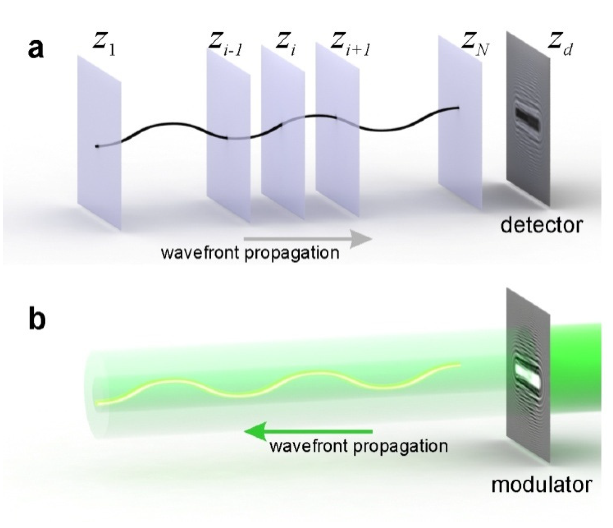
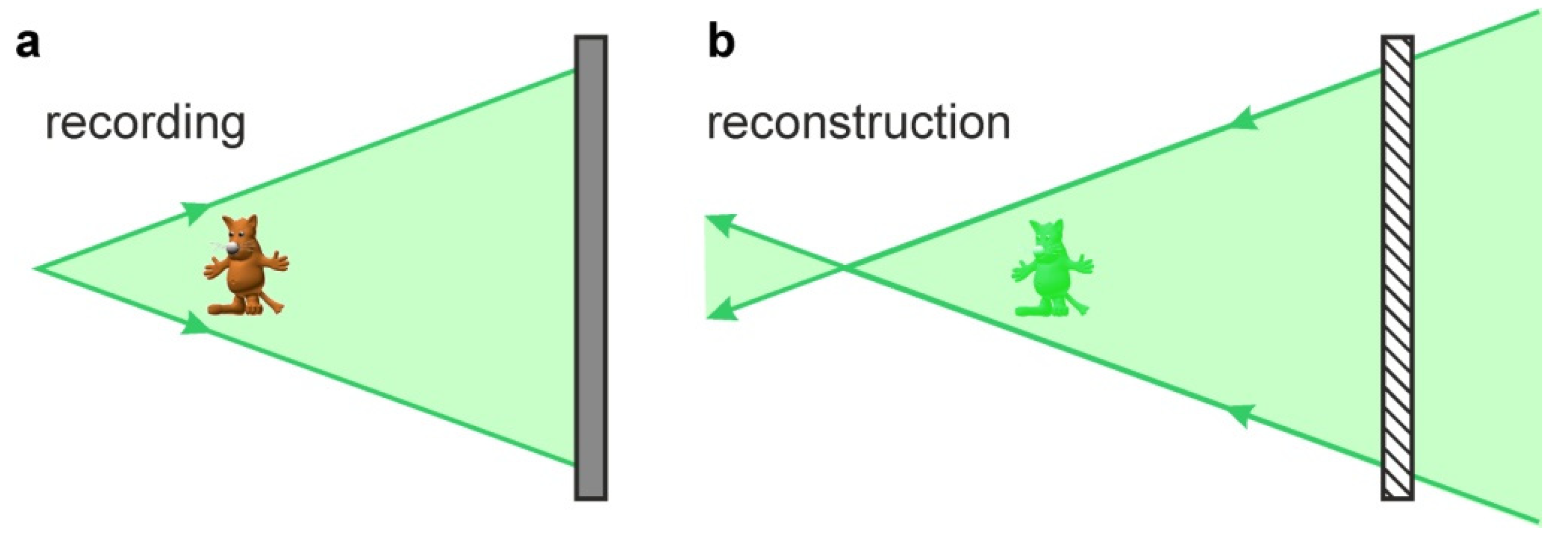
2.1. Principle of Arbitrary 3D Wavefront Modulation by Inverted Gabor Holography

The principle of creating arbitrary 3D intensity wavefront modulation is based on representing the 3D curve as a set of point-like absorbers closely packed to form a smooth version of the desired 3D curve. A hologram of such a 3D curve is simulated by propagating the wavefront through the planes, each containing one individual absorber. When such a hologram is reconstructed, a 3D curve made of absorbers is restored. When the contrast of the hologram is inverted, a 3D curve made of sources (instead of absorbers) is restored, thus forming a desired 3D intensity distribution. The details of the method are provided elsewhere [7]. Here we present the main steps, which are necessary for the rest of the manuscript, also illustrated in Figure 1:
(1) A set of planes along the z-axis is created at z i , i = 1 N . Each plane intersects the 3D curve at a point ( x 0 , y 0 , z i ) , as shown in Figure 1a. Each such point is considered to be a point-like absorber, and for each plane at z i , an object function is assigned o i ( x i , y i , z i ) such that
o i ( x , y , z i ) = { 0 , x x 0 , y y 0 1 , x = x 0 , y = y 0 .
Then, for each plane z i , a transmission function is assigned t i ( x i , y i , z i ) = 1 o i ( x i , y i , z i ) so that:
t i ( x , y , z i ) = { 1 , x x 0 , y y 0 0 , x = x 0 , y = y 0 .
(2) A plane wave illuminates the first plane at z 1 . The wavefront behind the first plane is given by the product of the incident wavefront and the transmission function of the first layer: u 1 ( x , y , z 1 ) = t 1 ( x , y , z 1 ) u 1 ( x , y , z 1 ) = t 1 ( x , y , z 1 ) . Next, the wavefront propagates to the plane z 2 , the propagation is calculated by using the angular spectrum method [20,21,22]:
u 2 ( x , y , z 2 ) = FT 1 { FT [ u 1 ( x , y , z 1 ) ] exp [ 2 π i ( z 2 z 1 ) λ 1 ( λ f x ) 2 ( λ f y ) 2 ] } ,
where FT and FT 1 denote the 2D Fourier and inverse Fourier transforms, respectively, ( f x , f y ) are the spatial frequencies, and λ is the wavelength. In the second plane, the wavefront u 2 ( x , y , z 2 ) is multiplied with the transmission function of the second plane, giving the wavefront right behind the second plane u 2 ( x , y , z 2 ) = t 2 ( x , y , z 2 ) u 2 ( x , y , z 2 ) , and so forth. After passing through the last Nth plane, the wavefront is propagated to the detector plane for a ( z d z N ) distance giving U ( X , Y ) , and the hologram H ( X , Y ) is calculated as H ( X , Y ) = | U ( X , Y ) | 2 .
(3) The obtained hologram H ( X , Y ) is reconstructed by illuminating it with a plane wave, and propagating the obtained wavefront backward through the object planes. The reconstructed wavefront will include the images of all the absorbers, that is, the points of zero-intensity, which will be arranged into the pre-defined 3D curve.
(4) The modulator is simulated as a contrast-inverted hologram:
M ( X , Y ) = 1 H ( X , Y ) ,
where H ( X , Y ) is the hologram distribution with its values normalized to be within the range of 0 to 1. Now, when modulator M ( X , Y ) is illuminated with a plane wave, the wavefront behind the modulator will recreate the contrast-inverted images of the absorbers, that is, the images of points of high intensity, which are arranged into the 3D intensity curve, as illustrated in Figure 1b. Thus, a pre-defined 3D beam of intensity will be formed.
Although in the original publication [7] this method was called “inverted Gabor holography”, the type of holography does not need to be Gabor type. The same principle of modeling intensity into a pre-defined 3D path can be achieved with other types of holography, for example, off-axis holography. For this reason, we will refer to the technique as simply “inverted holography”. Note that without inversion of the contrast of the hologram, the method of creating an arbitrary 3D curve will not work. It is impossible to simulate a hologram of bright sources, because in this case the transmission functions in each plane t i ( x , y , z i ) would be t i ( x , y , z i ) = 0 everywhere except the position of the source where t i ( x , y , z i ) = 1 , and the propagating wavefront would be multiplied by functions consisting mainly of zeros at each plane.

2.2. Three-Dimensional Wavefront Modulation with Spherical Waves

This section addresses the question, what can be the minimal size of the created 3D intensity distributions. It is common knowledge that holography with spherical waves [1,2] allows magnification/de-magnification of imaged objects. A prominent example is in-line electron holography with spherical waves, where a divergent spherical electron wave illuminates a nanometer-sized object and a hologram is formed on a detector that is positioned a few centimeters away from the sample; the resulting hologram has the size of several centimeters, thus achieving a magnification of 105–106. [23,24]. Such holograms can be translated onto a spatial light modulator or a photo film slide and reconstructed using laser light. The size of the reconstructed object is scaled by the ratio of the electron and laser light wavelengths. Moreover, holograms created with plane waves can be reconstructed by illuminating with spherical waves and vice versa [21]. Thus, using spherical waves allows for de-magnification/magnification of the created 3D wavefront modulation structures.
Employing a divergent spherical wavefront allows obtaining centimeter-sized holograms even for micro-sized objects. The centimeter-range size of the obtained hologram is sufficiently large to load the obtained hologram onto a spatial light modulator or to manufacture the hologram as a mask by using micro-fabrication techniques. The modulator is created by following the steps described above, and the incident wavefront is not a plane wave but a divergent spherical wave:
u 1 ( x , y , z 1 ) = exp [ i π λ z 1 ( x 2 + y 2 ) ] .
In the reconstruction step, the distribution on the modulator should be illuminated with a convergent wave, which can be realized by either using a convergent wave or by placing a lens with the corresponding phase distribution in the plane of the modulator. In the reconstruction process, the wavefront behind the modulator will converge to the object distribution, as illustrated in Figure 2.

2.3. Resolution

The lateral and axial resolutions ( R x , y and R z , respectively) of the created 3D wavefront structures formed using either plane or spherical waves are given by the Abbe criteria [25,26,27,28]:
R x , y = λ 2 NA ,
R z = 2 λ NA 2 ,
where NA is the numerical aperture of the optical setup:
NA S 2 z ,
S × S is the screen size and z is the sample-to-hologram distance for the plane waves and source-to-hologram distance for the spherical waves. Here it should be noted that the lateral resolution given by Equation (6) should be multiplied by a factor of 2 in the case of numerical reconstruction of a digital hologram due to the requirement of having at least two pixels to resolve two points. However, since in 3D wavefront modulation the “reconstruction” is not happening in a computer but it is happening in an reality, the formed 3D distribution does not need to be digitally sampled. The geometrical parameters of the setup can be optimized to maximize NA, but the fundamental limit of the resolution, and thus of the created 3D wavefront structures sizes, is given by the wavelength of the employed radiation.

3. Results

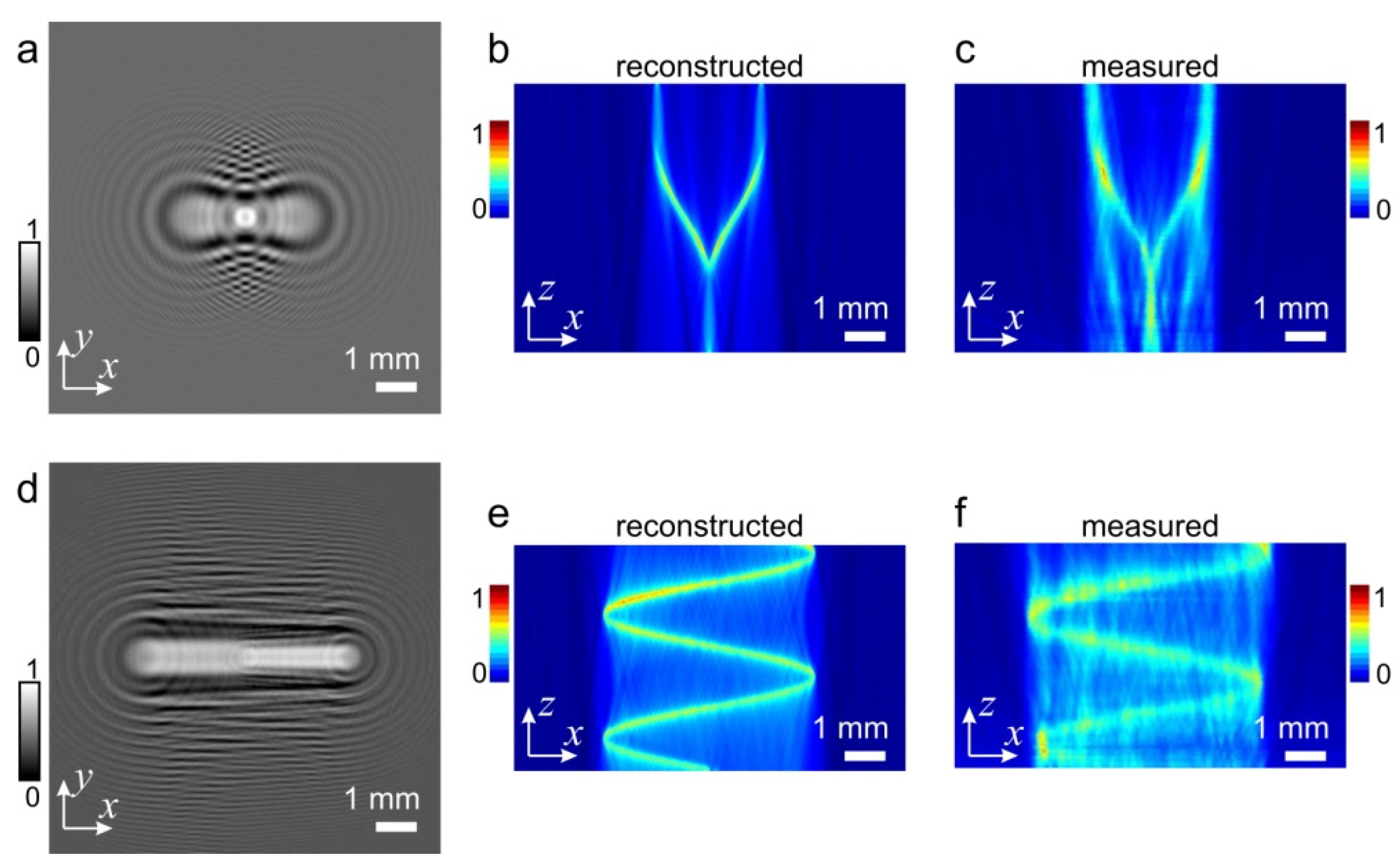
3.1. Three-Dimensional Intensity Wavefront Modulation Using Amplitude-Only Modulator

The method of inverted holography can be realized with any type of modulator or mask: amplitude-only, phase-only or a mixed type. In the original publication [7], an amplitude-only mask was considered, and several examples of 3D wavefront modulation were demonstrated: beam splitting, cosine-like, helical, etc. [7]; examples of beam-splitting and cosine-like 3D intensity curves are shown in Figure 3. Three-dimensional wavefront intensity modulation using an amplitude-only modulator is the most straightforward approach because it directly applies the holographic principle and uses a contrast-inverted hologram distribution as the modulator distribution. Three-dimensional wavefront intensity modulation using an amplitude-only modulator was previously discussed in great detail in the original publication [7], and therefore it is not discussed in this paper.

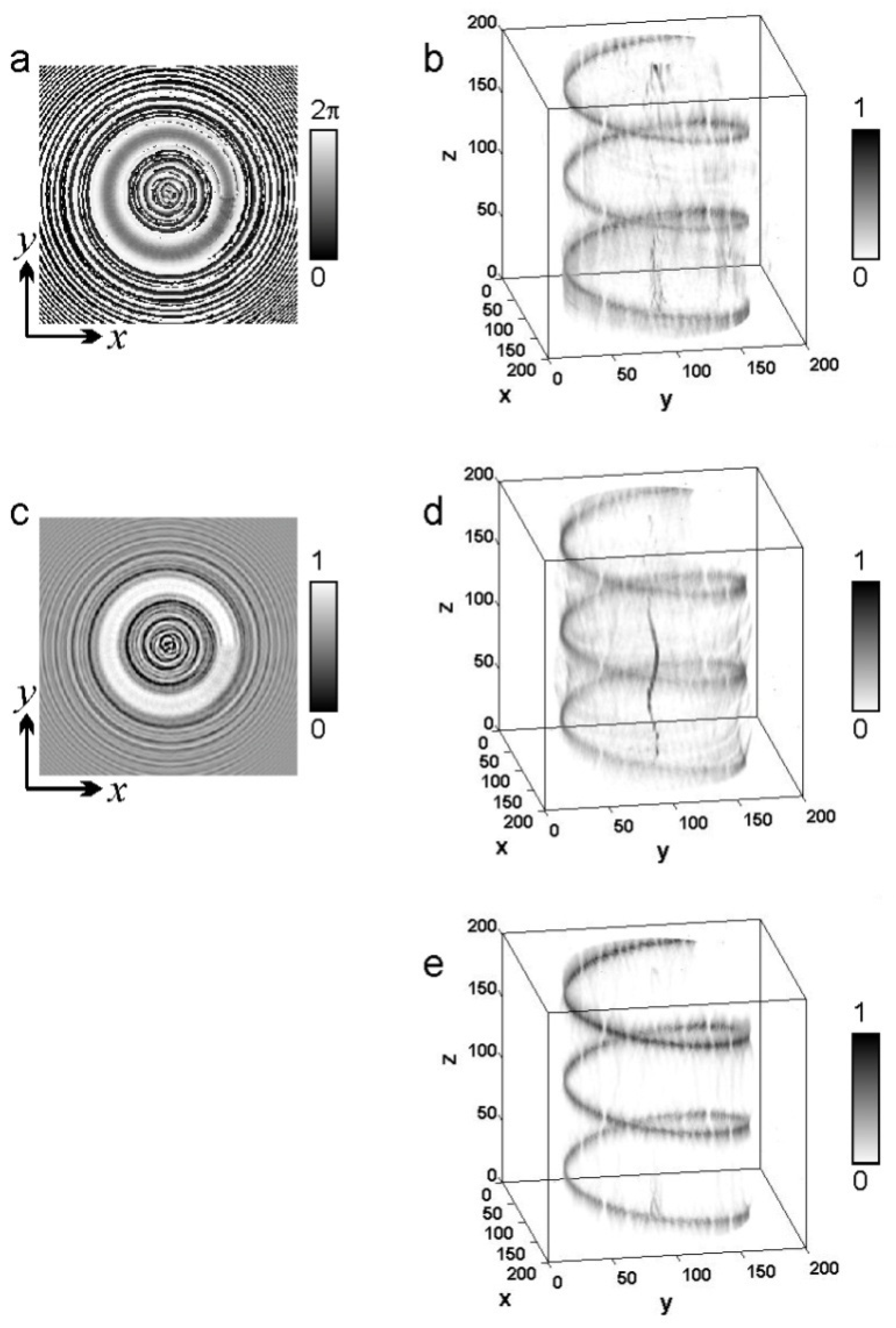
3.2. Three-Dimensional Intensity Wavefront Modulation Using Phase-Only Modulator

In some applications only phase modulation is possible. In this case, 3D intensity wavefront modulation can also be conducted using a phase-only modulator. A review of the most effective methods of 2D wavefront modulation using phase-only modulators is provided by Clark et al. [29]. Here we demonstrate a method that we found the most effective for 3D wavefront intensity modulation. To illustrate the method, we created a 3D intensity beam in the form of a 3D helix with a radius of 70 pixels and a period of 70 pixels, sampled with 200 × 200 × 200 pixels. In the simulations, we used the same parameters as previously used in the optical experiments in reference [7]: wavelength = 650 nm, the transmission functions and the modulator distribution were sampled with 832 × 832 pixels, the pixel size in the (x, y)-plane was Δx,y = 32 μm. A total of 200 sampling planes along the z-axis with the distance between two adjacent planes of Δz = 4 mm were applied, so that the total length of the 3D curve was 4 mm × 200 = 800 mm. The distance between the last plane and the detector plane was z0 = 100 mm.
The corresponding transmission functions of each of the 200 planes were calculated as described above. For each plane, its transmission function was formed as described by Equations (1) and (2). The obtained 3D array of transmission functions was blurred by convolution with a Gaussian distribution exp [ ( i i 2 + j j 2 + k k 2 ) ] with the standard deviation of 1 / 2 pixel, where ii, jj, kk are the pixel numbers. After the wavefront had been propagated through all the planes and to the detector, the complex-valued distribution in the detector plane U ( X , Y ) was obtained. The phase of the obtained distribution U ( X , Y ) was corrected by adding a constant phase shift such that the phase of the reference wave was zero: U ( X , Y ) U ( X , Y ) exp [ i 2 π λ ( z d z 1 ) ] . The phase-only modulator distribution was calculated as:
M ( X , Y ) = exp { i Arg [ U ( X , Y ) + C ] } ,
where C is a small constant. The best results were obtained with C = 0.8, which was discovered out by trying different values of C. The physical meaning of adding the constant can be explained as follows. The distribution U ( X , Y ) is given by the plane wave propagating through an array of absorbers and can be written as U ( X , Y ) = 1 O ( X , Y ) , where one describes the plane wave and O ( X , Y ) describes the wavefront due to the absorbers. This gives U ( X , Y ) + C = O ( X , Y ) + ( C 1 ) , where the first term O ( X , Y ) reconstructs the signal from the absorbers with a positive sign, thus giving the point sources, and ( C 1 ) is that constant with a value close to zero, which should reconstruct background signal. The best contrast of the obtained 3D curve was obtained with C = 0.8 and not with C = 1, as one would expect. The result cannot be explained at this point.
The calculated phase distribution of the modulator is shown in Figure 4a and the obtained 3D intensity beam is shown in Figure 4b. The lateral and axial resolution evaluated with Equations (6) and (7) for wavelength = 650 nm, the total area of 26.624 mm × 26.624 mm, and z = 100 mm (the distance from the last plane to the detector), amount to R x , y = 2.5 μm and R z = 76.0 μm, respectively. For comparison, identically shaped 3D intensity beams were created using an amplitude-only modulator (calculated as described above using Equation (4) and shown in Figure 4c) and a complex-valued modulator calculated as
M ( X , Y ) = 1 U ( X , Y ) .
The obtained intensity distributions are shown in Figure 4d and Figure 4e, respectively. It must be noted that the method based on using a phase-only modulator is not necessarily a better method than the method based on using an amplitude-only modulator. However, in some applications only phase-only modulators are available, and they were not considered in the original publication [7].
From comparing the results shown in Figure 4, the following observations can be made: both methods, based on using amplitude-only and phase-only modulators, demonstrate artifacts when compared to the result obtained using a perfect complex-valued modulator. The 3D intensity beam obtained using a phase-only modulator does not exhibit a strong artifact at the optical axis, which can be an artifact only specific for a helical curve and might not be present for other 3D curves. The smoothness of the 3D curves, given by the x, y, and z-resolution, is the same for all three 3D curves. In the next section, it is shown that the smoothness can be enhanced by using finer sampling.

3.3. High-Resolution Modulator

In order to achieve a smoother appearance of the created 3D intensity curves, more sampling pixels in all three dimensions should be used. It has been previously demonstrated that when 2000 slices along the z-axis are employed instead of 200 slices, the formed 3D intensity curve has a smoother appearance [7]. In addition, a higher number of pixels and a smaller pixel size can be employed, which we investigate here. A high-resolution 3D helical intensity beam was obtained using a simulated phase-only modulator with the same area of 26.624 mm × 26.624 mm but sampled with 2000 × 2000 pixels. The created helix was 375 pixels in radius with a period of 5600 pixels. The total length of the 3D helical curve was 100 mm, and it was sampled with 16,000 planes along the z-axis. The 2D transmission functions of each plane were blurred by using convolution with a blurring kernel
( 1 1 1 1 4 1 1 1 1 ) .
The distance from the last plane to the detector was 200 mm.
The distribution of the modulator was obtained by using Equation (9). It took about 6 h to compute such a high-resolution diffractor on a PC with Intel(R) Core(TM) i7-2600 CPU @ 3.40 GHz and 16 GB RAM.
Once the high-resolution distribution of the phase-only modulator is calculated (Figure 5a), the 3D curve can be restored by using this modulator at different parameters. Two sets of parameters are shown in Figure 5b,c. In the example shown in Figure 5b, the 3D intensity curve was restored by re-sampling the distribution of the phase-only modulator from 2000 × 2000 pixels to 832 × 832 pixels. The re-sampling was conducted as follows. The real and imaginary parts of the complex-valued distribution U ( X , Y ) each were re-sampled separately by using a quadratic interpolation formula to compute the pixel location and then the resulting distributions were recombined into the re-sampled complex-valued U ( X , Y ) . The phase-only modulator was calculated using Equation (9). In the example shown in Figure 5c, the curve was restored using the phase-only modulator sampled with the entire range of 2000 × 2000 pixels. From comparing Figure 5b,c, it is apparent that the 3D intensity curve obtained from the modulator sampled with a higher number of pixels (2000 × 2000 pixels) exhibits a smoother appearance. The lateral and axial resolutions evaluated with Equations (6) and (7) for wavelength = 650 nm, the total area of 26.624 mm × 26.624 mm, and z = 200 mm, amount to R x , y = 4.9 μm and R z = 296.0 μm, respectively. These resolutions are independent of the number of pixels or the pixel size and are the same for both 3D curves shown in Figure 5b,c. The limited z-resolution explains that the created 3D intensity curve exhibits some thickness in the z-direction. A slight increase in intensity towards a larger distance of z can be equalized by adjusting the object functions in each plane, as given by Equation (1), so that o i ( x i , y i , z i ) = 0 everywhere except the position of the point-like absorber where o i ( x i , y i , z i ) = a , where a is a constant that defines the strength of the resulting intensity, where a = 1 for the maximal intensity. a can be selected to gradually decrease from a = 1 for smaller z-distances to a < 1 for larger z-distances.

4. Discussion

In conclusions, a more comprehensive study of 3D wavefront modulation by using contrast-inverted holograms was presented. Three-dimensional 3D wavefront modulation by using a phase-only modulator was demonstrated. From comparing the results obtained by using an amplitude-only vs a phase-only only modulators, the following conclusions can be made: both methods demonstrate a similar quality of the created 3D intensity beams with some artifacts at the optical axis when compared to the intensity beam obtained using a perfect complex-valued modulator. The smoothness of the 3D curves, given by the x, y, and z-resolution, is the same for 3D curves created using amplitude-only, phase-only and complex-valued modulators. The smoothness of the formed 3D intensity curves is given by the sampling parameters when simulating the diffractor distribution: the number of pixels and the pixel size in all the dimensions, the number of pixels of the employed modulator and its pixel size. Both the resolution and the size of the created 3D wavefront intensity structure are given by the classical resolution criteria and ultimately are limited by the wavelength of the employed radiation. Three-dimensional intensity beams can be created by using a spherical wavefront that allows focusing the wavefront into a localized intense distribution and, therefore, can be employed for miniaturization of the produced 3D intensity beams. Three-dimensional wavefront intensity structures can be used for various applications: 2D and 3D lithography, optical tweezers, etc. For example, 3D lithography of small 3D structures can be utilized for the mass-production of micro-robots [30,31]. Three-dimensional wavefront intensity modulation into an arbitrary 3D distribution can be realized for various waves: light, X-ray, electrons, etc. provided that the modulator can be manufactured at the corresponding wavelength.

Funding

This research received no external funding.

Institutional Review Board Statement

Not applicable.

Informed Consent Statement

Not applicable.

Data Availability Statement

No new data were created or analyzed in this study. Data sharing is not applicable to this article.

Acknowledgments

Financial support of the University of Zurich is acknowledged.

Conflicts of Interest

The authors declare no conflict of interest.

References

  1. Gabor, D. A new microscopic principle. Nature 1948, 161, 777–778. [Google Scholar] [CrossRef] [PubMed]
  2. Gabor, D. Microscopy by reconstructed wave-fronts. Proc. R. Soc. Lond. A 1949, 197, 454–487. [Google Scholar] [CrossRef]
  3. Tricoles, G. Computer generated holograms—An historical review. Appl. Opt. 1987, 26, 4351–4360. [Google Scholar] [CrossRef] [PubMed]
  4. Bryngdahl, O.; Wyrowski, F. Digital holography-computer-generated holograms. Prog. Opt. 1990, 28, 1–86. [Google Scholar] [CrossRef]
  5. Skeren, M.; Richter, I.; Fiala, P. Design of binary phase-only diffractive optical elements for laser beam shaping. In Laser Beam Shaping; Dickey, F.M., Holswade, S.C., Eds.; Spie-Int Soc Optical Engineering: Bellingham, WA, USA, 2000; Volume 4095, pp. 154–164. [Google Scholar]
  6. Yu, W.J.; Takahara, K.; Konishi, T.; Yotsuya, T.; Ichioka, Y. Fabrication of multilevel phase computer-generated hologram elements based on effective medium theory. Appl. Opt. 2000, 39, 3531–3536. [Google Scholar] [CrossRef]
  7. Latychevskaia, T.; Fink, H.-W. Inverted Gabor holography principle for tailoring arbitrary shaped three-dimensional beams. Sci. Rep. 2016, 6, 26312. [Google Scholar] [CrossRef] [Green Version]
  8. Latychevskaia, T.; Schachtler, D.; Fink, H.-W. Creating Airy beams employing a transmissive spatial light modulator. Appl. Opt. 2016, 55, 6095–6101. [Google Scholar] [CrossRef]
  9. Shiloh, R.; Arie, A. 3D shaping of electron beams using amplitude masks. Ultramicroscopy 2017, 177, 30–35. [Google Scholar] [CrossRef] [Green Version]
  10. Gerchberg, R.W.; Saxton, W.O. A practical algorithm for determination of phase from image and diffraction plane pictures. Optik 1972, 35, 237–246. [Google Scholar]
  11. Fienup, J.R. Iterative method applied to image-reconstruction and to computer-generated holograms. Opt. Eng. 1980, 19, 297–305. [Google Scholar] [CrossRef]
  12. Berry, M.V.; Balazs, N.L. Nonspreading wave packets. Am. J. Phys. 1979, 47, 264–267. [Google Scholar] [CrossRef]
  13. Siviloglou, G.A.; Broky, J.; Dogariu, A.; Christodoulides, D.N. Observation of accelerating Airy beams. Phys. Rev. Lett. 2007, 99, 213901. [Google Scholar] [CrossRef] [PubMed]
  14. Rodrigo, J.A.; Alieva, T.; Abramochkin, E.; Castro, I. Shaping of light beams along curves in three dimensions. Opt. Express 2013, 21, 20544–20555. [Google Scholar] [CrossRef] [PubMed] [Green Version]
  15. Voloch-Bloch, N.; Lereah, Y.; Lilach, Y.; Gover, A.; Arie, A. Generation of electron Airy beams. Nature 2013, 494, 331–335. [Google Scholar] [CrossRef] [PubMed] [Green Version]
  16. Lee, S.H.; Roichman, Y.; Grier, D.G. Optical solenoid beams. Opt. Express 2010, 18, 6988–6993. [Google Scholar] [CrossRef] [Green Version]
  17. Brzobohaty, O.; Karasek, V.; Siler, M.; Chvatal, L.; Cizmar, T.; Zemanek, P. Experimental demonstration of optical transport, sorting and self-arrangement using a ‘tractor beam’. Nature Photon. 2013, 7, 123–127. [Google Scholar] [CrossRef] [Green Version]
  18. Rosen, J.; Yariv, A. Snake beam—A paraxial arbitrary focal line. Opt. Lett. 1995, 20, 2042–2044. [Google Scholar] [CrossRef] [Green Version]
  19. Latychevskaia, T.; Fink, H.-W. Inverted Gabor holography principle for tailoring arbitrary shaped three-dimensional beams: Matlab code. Matlab File Exch. Server. 2016. Available online: https://ch.mathworks.com/matlabcentral/fileexchange/92218-92213d-wavefront-modulation-by-inverted-gabor-holography (accessed on 22 May 2021).
  20. Ratcliffe, J.A. Some aspects of diffraction theory and their application to the ionosphere. Rep. Prog. Phys. 1956, 19, 188–267. [Google Scholar] [CrossRef]
  21. Latychevskaia, T.; Fink, H.-W. Practical algorithms for simulation and reconstruction of digital in-line holograms. Appl. Opt. 2015, 54, 2424–2434. [Google Scholar] [CrossRef] [Green Version]
  22. Goodman, J.W. Introduction to Fourier Optics, 3rd ed.; Roberts & Company Publishers: Greenwood Village, CO, USA, 2004. [Google Scholar]
  23. Fink, H.-W.; Stocker, W.; Schmid, H. Holography with low-energy electrons. Phys. Rev. Lett. 1990, 65, 1204–1206. [Google Scholar] [CrossRef] [Green Version]
  24. Fink, H.-W.; Schmid, H.; Ermantraut, E.; Schulz, T. Electron holography of individual DNA molecules. J. Opt. Soc. Am. A 1997, 14, 2168–2172. [Google Scholar] [CrossRef]
  25. Abbe, E. On the estimation of aperture in the microscope. J. R. Microsc. Soc. 1881, 1, 388–423. [Google Scholar] [CrossRef]
  26. Abbe, E. The relation of aperture and power in the microscope. J. R. Microsc. Soc. 1882, 2, 300–309. [Google Scholar] [CrossRef] [Green Version]
  27. Latychevskaia, T.; Longchamp, J.-N.; Fink, H.-W. When holography meets coherent diffraction imaging. Opt. Express 2012, 20, 28871–28892. [Google Scholar] [CrossRef] [PubMed] [Green Version]
  28. Latychevskaia, T. Lateral and axial resolution criteria in incoherent and coherent optics and holography, near- and far-field regimes. Appl. Opt. 2019, 58, 3597–3603. [Google Scholar] [CrossRef] [PubMed] [Green Version]
  29. Clark, T.W.; Offer, R.F.; Franke-Arnold, S.; Arnold, A.S.; Radwell, N. Comparison of beam generation techniques using a phase only spatial light modulator. Opt. Express 2016, 24, 6249–6264. [Google Scholar] [CrossRef] [PubMed] [Green Version]
  30. Nelson, B.J.; Kaliakatsos, I.K.; Abbott, J.J. Microrobots for minimally invasive medicine. In Annual Review of Biomedical Engineering; Yarmush, M.L., Duncan, J.S., Gray, M.L., Eds.; Annual Reviews: Palo Alto, CA, USA, 2010; Volume 12, pp. 55–85. [Google Scholar]
  31. Huang, H.W.; Sakar, M.S.; Petruska, A.J.; Pane, S.; Nelson, B.J. Soft micromachines with programmable motility and morphology. Nat. Commun. 2016, 7, 1–10. [Google Scholar] [CrossRef] [Green Version]
Figure 1. Three-dimensional wavefront modulation by inverted holography principle. (a) A pre-defined 3D curve is sampled in the planes at z i , i = 1 N , providing a distribution of transmission functions t i ( x , y , z i ) . Hologram H ( X , Y ) is simulated by propagating the plane wave through all the planes down to the hologram plane ( X , Y ) . (b) Reconstruction of the 3D light curve. A plane wave illuminates the modulator M ( X , Y ) , which is a contrast-inverted hologram, and the wavefront behind the modulator is shaped into a 3D intensity distribution. Adapted from [7].
Photonics 08 00179 g001
Figure 2. In-line holography with spherical waves. (a) In the recording, the object is illuminated with a divergent spherical wave. (b) In the reconstruction, the hologram is illuminated with a convergent spherical wave, and the wavefront behind the hologram converges to the original object distribution.
Photonics 08 00179 g002
Figure 3. Three-dimensional intensity wavefront modulation employing amplitude-only modulator, simulation and experimental results. (ac) Three-dimensional intensity wavefront modulation in the form of a splitting beam. (df) Three-dimensional intensity wavefront modulation in the form of a cosine-like curve. (a,d) Amplitude distributions loaded on an amplitude-only transmissive modulator, only the central regions, 300 × 300 pixels of 832 × 832 pixels, are shown. (b,e) Obtained 3D intensity distribution behind the modulator, the pixel size in the (x, y) plane Δx,y = 32 μm, pixel size along z-axis Δz = 4 mm, total z-range is 800 mm. (c,f) Experimentally measured intensity distributions behind the modulator. Adapted from [7].
Photonics 08 00179 g003
Figure 4. Three-dimensional intensity wavefront modulation in the form of a 3D helical structure employing a phase-only modulator, simulated study. (a) Phase distribution loaded on a phase-only modulator, only the central region of 300 × 300 pixels of 832 × 832 pixels is shown. (b) Three-dimensional intensity distribution reconstructed behind the modulator. (c) Amplitude distribution loaded on an amplitude-only modulator, only the central region of 300 × 300 pixels of 832 × 832 pixels is shown, and (d) 3D intensity distribution reconstructed behind an amplitude-only modulator. (e) Three-dimensional intensity distribution reconstructed behind a complex-valued modulator. For all three modulators: pixel size in the (x, y) plane is Δx,y = 32 μm, pixel size along the z-axis is Δz = 4 mm, total length along the z-axis is 800 mm.
Photonics 08 00179 g004
Figure 5. Three-dimensional intensity helical structure obtained by using a phase-only modulator calculated with 2000 × 2000 pixels, simulated study. (a) The phase distribution of the modulator. (b) The intensity distribution of the 3D helical curve obtained from the modulator distribution sampled with 832 × 832 pixels. (c) The intensity distribution of the 3D helical curve obtained from the modulator distribution sampled with 2000 × 2000 pixels.
Photonics 08 00179 g005
Publisher’s Note: MDPI stays neutral with regard to jurisdictional claims in published maps and institutional affiliations.

