Enhancing Multi-Distance Phase Retrieval via Unequal Interval Measurements

Abstract

In the conventional methods of multi-distance phase retrieval, the diffraction intensity patterns are recorded at equal intervals, which can induce slow convergence or stagnation in the subsequent reconstruction process. To solve this problem, a measurement method with unequal intervals is proposed in this paper. The interval spacings between adjacent measurement planes are decreased gradually. A large gap accelerates retrieval progress, and a short span helps to recover detailed information. The proposed approach makes full use of the available measured dataset and simultaneously generates variations in diversity amplitude, which is a crucial issue for the techniques of multi-image phase retrieval. Both computational simulations and experiments are performed. The results demonstrate that this method can improve the convergence speed by 2 to 3 times and enhance the quality of reconstruction results in comparison to that of the conventional methods.

1. Introduction

Generally speaking, image sensors are sensitive to the wavefield intensity. However, they cannot obtain phase distribution, which is more important in the imaging of some transparent samples. To address this problem, the phase retrieval algorithm was proposed [1,2,3]. This is a type of technique to reconstruct the wavefront without interferometric measurement. This technique is intended to acquire the lost wavefront during the detection process and calculate the wavefront directly using the known measured intensity. It significantly simplifies the experimental setup and reduces the experimental cost. To date, phase retrieval has been successfully applied to the imaging of biological cells [4,5], tomographic imaging [6,7], super-resolution imaging [8,9], and other research fields.

A pioneering work in phase retrieval is represented by the Gerchberg–Saxton (GS) algorithm [10]. This is a double-intensity iterative algorithm that only demands one recording plane. The GS algorithm works by means of calculating the wave diffraction propagations between the recording plane and the object plane. In the GS algorithm, the retrieval begins with an assumed field at the object plane. Then, the complex field propagates to the observed plane, where the amplitude of the spread light field is substituted by the measured values. Subsequently, the modified light distribution propagates backward to the object plane, where the guessing phase is updated. The algorithm recovers the target phase by continuously performing the transmission of double directions. However, it is easy to drop into the local minimum and difficult to reach the desired global optimal solution due to the inadequate constraints. Moreover, the problem of stagnation exists in the propagation process. Several improved methods have been introduced in the literature to overcome this weakness, such as defining a support area in the object domain [11,12] and optimizing the amplitude constraint conditions [13,14]. Nevertheless, only relying on the information provided by a single measured value results in the problems of convergence precision and low speed, and it is difficult to fulfil the expected requirements. Consequently, multi-intensity measurements have been proposed [15,16,17,18]. In these approaches, a set of amplitude or phase modulations are added sequentially between the recording plane and the object plane. Then, the data of multiple diffraction intensity are orderly recorded on one measured plane. Modulations are employed so as to enhance the intensity variation and generate a fast convergence rate and a high-quality image. However, all these methods require additional equipment, such as a mask, phase plate, and spatial light modulator (SLM), and entail extra costs, complicating the optical platform accordingly.

To avoid a complicated experimental setup and redundant noise generated from the modulations, a single-beam multiple-intensity reconstruction (SBMIR) algorithm has been proposed [19,20]. This technique exploits multiple diffractive patterns which are successively measured at diverse distances downstream of the illuminated sample with the same interval step. Adapting the technique of amplitude replacement in the GS algorithm, SBMIR with multi-constraints gradually updates the target phase value when the light beam passes through each observation plane. However, some smooth samples produce a weak difference in diffraction intensity among the measurement planes. Moreover, the iterative method suffers from low convergence speed because the key issue in valid phase recovery is sufficient intensity variation. To facilitate a change in the diffraction intensity received by the sensor, speckle illumination [21,22,23,24,25,26,27,28,29,30,31,32] was proposed on the basis of SBMIR. However, speckle noise will cause aliasing and leakiness during the final reconstructions. To avoid systematic noise, some methods are employed in order to improve the SBMIR algorithm without extra equipments. One of the extended techniques is that which enhances the phase retrieval by means of establishing an intermediate virtual plane between the object plane and the initially measured plane [33]. Another method has been proposed to propagate the wavefront in an unordered sequence [34]. This strategy significantly increases the number of potential means of wavefield transmission which stimulate the change in amplitude. Meanwhile, in SBMIR, the information difference between two adjacent planes is very small, which leads to the accumulation of redundant noise and affects the accuracy of the reconstruction.

In this study, a straightforward technique based on unequal interval measurements for enhanced multi-distance phase retrieval is proposed. The distinct difference from the SBMIR is that our proposed technique allows the measured planes to be set with unequal intervals. The large wave propagation distance averages the noise accumulation and provides several datasets with less similarity, accelerating the convergence speed accordingly. The small span of transmission helps to recover the high frequency of the object, which indicates the potential ability to realize the precision of reconstruction. With the same number of planes and iterations, our method performs significantly in terms of reconstruction quality and convergence speed through simulations and experiments. Additionally, the reconstruction error caused by the change in insufficient intensity using the equal interval measurements can be promptly corrected through the unequal interval algorithm.

2. Methods

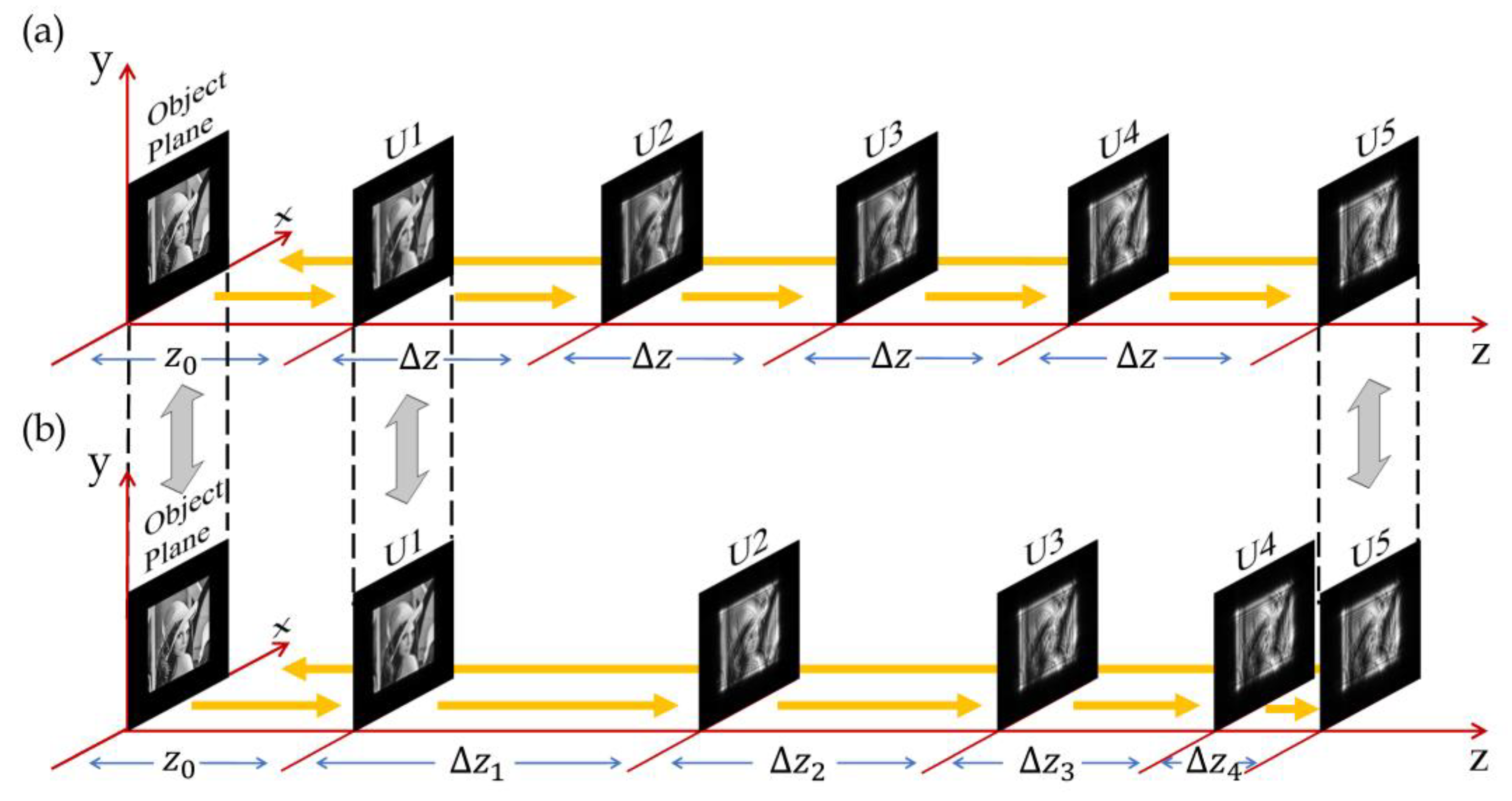
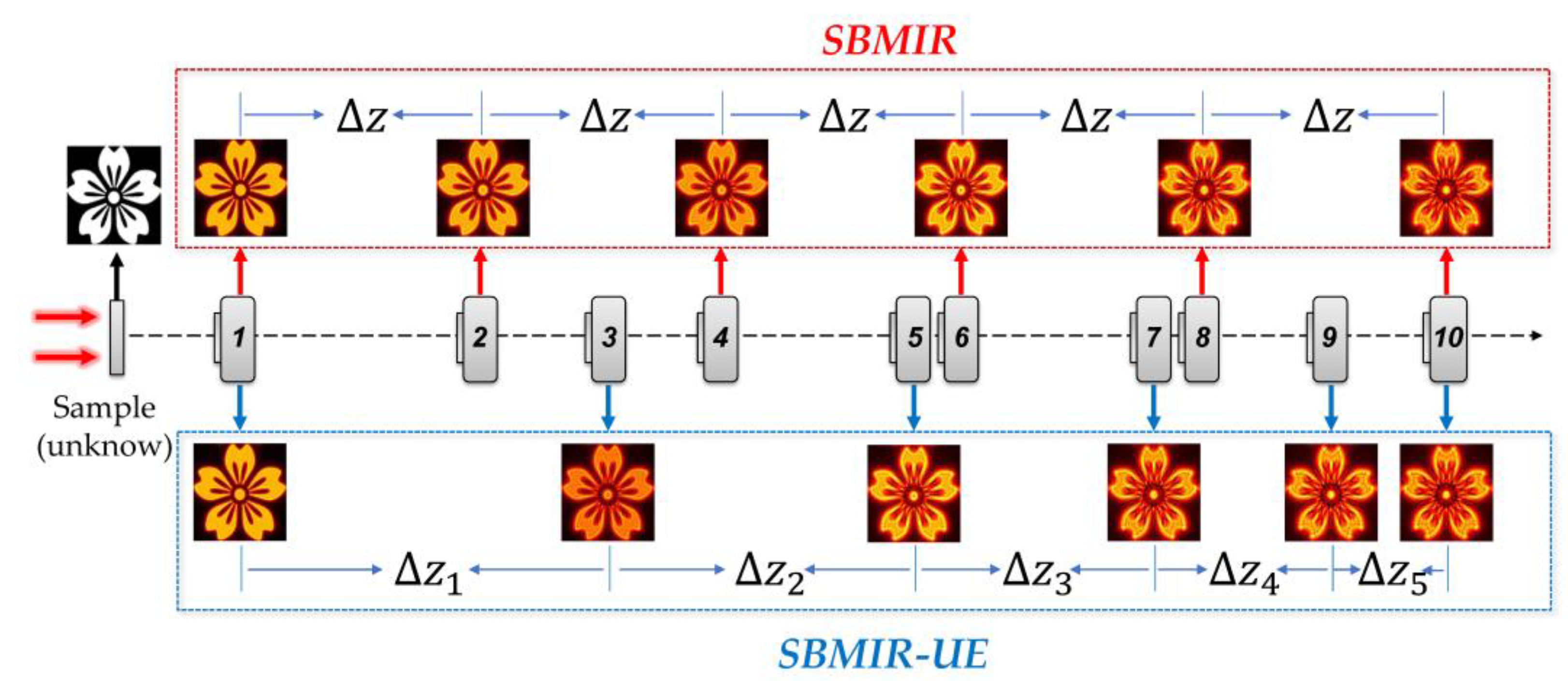
Figure 1 shows the schematic diagram of the conventional equal interval method (SBMIR) and our proposed unequal interval method (referred to as SBMIR-UE hereinafter). SBMIR is shown in Figure 1a. The sample is placed on the object plane and illuminated by the coherent laser beam. Then, the diffraction intensities are recorded using a charge coupled device (CCD) sensor. The CCD is initially located in the first plane U1 and the initial distance from the object plane is z₀. Subsequently, it is successively shifted backward with the same interval Δz to complete the rest of the plane recordings.

The proposed SBMIR-UE is shown in Figure 1b. It can be seen that the interval step of several measurement planes varies from large distances such as Δz₁ to short distances such as Δz₄, which is not as uniform as that of SBMIR. The spacings are isometrically decreased. Δz_i−1 represents the interval space between adjacent planes U_i and U_i−1 and satisfies the following relationship:

$$\Delta z_{i-1}-\Delta z_i=d,$$

(1)

where d is a positive value. In these two methods, the wave propagations are calculated by the same equation, and the sequences of the transmission are indicated by the orange arrows, as shown in Figure 1. The only difference is the diffraction distance.

The iteration process of the two methods begins with an initially constant field at the object plane, and then the wavefront passes through the subsequent measured plane, where the calculated amplitude is replaced by the square root of the measured intensity, and the calculated phase is kept constant. When the wavefield reaches the last observation plane, it is inversely propagated to the object plane. The corresponding calculated complex amplitude is prepared for the next same iteration. The angular spectrum of scalar diffraction is used to calculate the diffraction as

$$A_{out}(x,y)=F^{-1}\{F[A_{in}(x,y)]v(\xi ,\eta )\},$$

(2)

where A_in is the complex field of the input plane, A_out the complex field of the output plane, (x, y) the spatial coordinates, F⁻¹ and F the positive and inverse Fourier transform, respectively, and v the transfer function for diffraction propagation with $\xi$ and $\eta$ as the coordinates in the frequency domain. The transfer function $v(\xi ,\eta )$ can be defined as

$$v(\xi ,\eta )=\{\begin{array}{cc}{e}^{\frac{j2\pi z}{\lambda }{[1-{(\lambda \xi )}^2-{(\lambda \eta )}^2]}^{\frac{1}{2}}},& {\xi }^2+{\eta }^2<\frac{1}{{\lambda }^2}\\ 0,& \mathrm{else}\end{array},$$

(3)

where z is the diffraction transmission distance and λ the wavelength of incident light. The mean square error (MSE) is used to evaluate the reconstructed result, which is defined as

$$MSE=\frac{1}{XY}{\displaystyle \sum _{x=1}^X{\displaystyle \sum _{y=1}^Y{[A(x,y)-{\widehat{A}}_c(x,y)]}^2}},$$

(4)

where $A(x,y)$, ${\widehat{A}}_{\mathrm{c}}(x,y)$, x and y represent the target distribution, the reconstruction results and the pixel values of the object plane in x- and y-directions, respectively.

3. Simulation

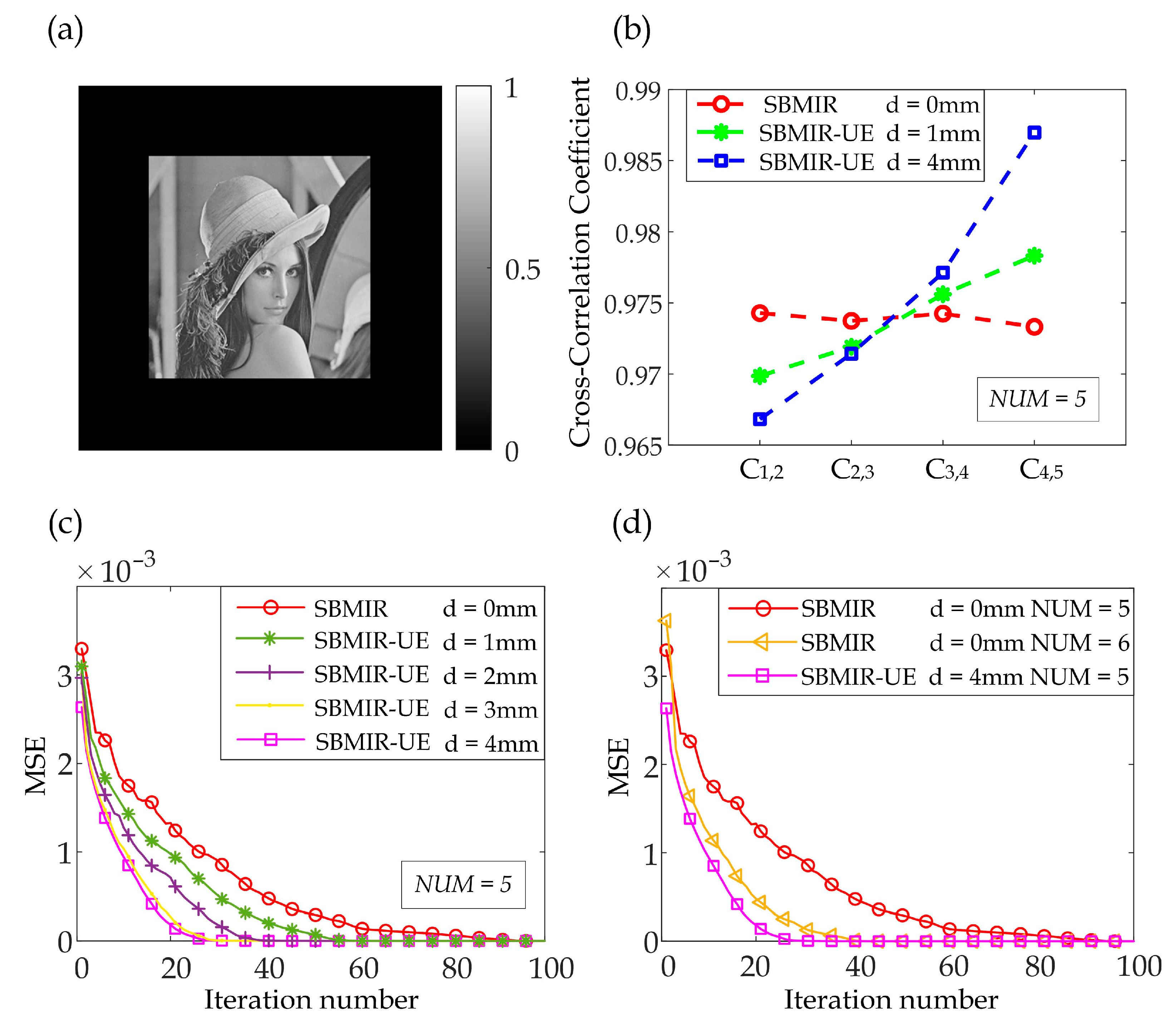
Numerical simulations are carried out for the purpose of comparing the performance of the two different methods. Here, we choose the image ‘’lena’’ (256 × 256 pixels) as the ground truth with the uniform phase. In the simulation, the image is padded with zeros to form 420 × 420 pixels, as shown in Figure 2a. Other parameters are set as follows: wavelength is λ = 650 nm, the initial distance between the target plane and the first measured plane is z₀ = 5 mm, the pixel size of the measured plane is 7.4 μm, the number of recording planes (NUM) is 5, the iteration number is 100, the initial phase is the uniform distribution, the interval between the adjacent planes in SBMIR is Δz = 7.5 mm. For SBMIR-UE, four groups of interval spaces are used: (1) d = 4 mm, Δz₁ = 13.5 mm, Δz₂ = 9.5 mm, Δz₃ = 5.5 mm, Δz₄ = 1.5 mm; (2) d = 3 mm, Δz₁ = 12 mm, Δz₂ = 9 mm, Δz₃ = 6 mm, Δz₄ = 3 mm; (3) d = 2 mm, Δz₁ = 10.5 mm, Δz₂ = 8.5 mm, Δz₃ = 6.5 mm, Δz₄ = 4.5 mm; and (4) d = 1 mm, Δz₁ = 9 mm, Δz₂ = 8 mm, Δz₃ = 7 mm, Δz₄ = 6 mm. It is worthwhile to point out that the object plane, first plane and last plane of the SBMIR coincide with those of the SBMIR-UE.

The convergence curves of SBMIR and SBMIR-UE are shown in Figure 2c. As the number of iterations increases, the value of MSE in both methods decreases gradually. Obviously, compared to the traditional method, the four cases of SBMIR-UE all converge rapidly. It can be seen that the greater the spacing difference, the faster the reconstruction will be. To visualize the data in Figure 2c,

Table 1. Convergence speed ratio of the two methods.

Performance	Unequal Measurements				Equal Measurements
d (mm)	1	2	3	4	0
Iteration times	58	40	31	28	94
Speed ratio	1.57	2.35	3.03	3.36	1.00

shows a comparison of required iteration times and the speed ratio for the two methods. The speed ratio is defined by the ratio of iteration times of SBMIR and SBMIR-UE. Meanwhile, the speed ratio of equal interval measurement is set to be 1.00. As can be seen, the conventional SBMIR converges 94 times, and the proposed SBMIR-UE with d = 4 mm converges 28 times. The convergence rate is improved by 3.36 times. Even when d = 1, 2 and 3 mm, iteration times of 58, 40 and 31 are sufficient to complete the iteration.

One may wonder why the proposed strategy is able to enhance the reconstructed results. To further explain the principle of our method, the cross-correlation of the intensity on the adjacent measurement planes was calculated and the result is presented in Figure 2b. The C_i,i+1 represents the cross-correlation coefficient between the planes U_i and U_i+1. The large coefficient indicates a slight intensity variation and a small value indicates a large intensity difference. It can be seen clearly that in the traditional method (red curve), the coefficient values are nearly the same, which indicates the minor intensity change among the measured planes, leading to the convergence stagnation of the iteration. In contrast, for the improved method (green and blue curves), the cross-correlation coefficients are changed clearly from small to large values, corresponding to the intensity variation varied from maximum to minimum. The large intensity difference benefits from long propagation distance, which promotes the rate of convergence. The large coefficient indicates that the two adjacent patterns are similar each other, which is helpful when making adjustments in detail and recovering the high frequency of the sample.

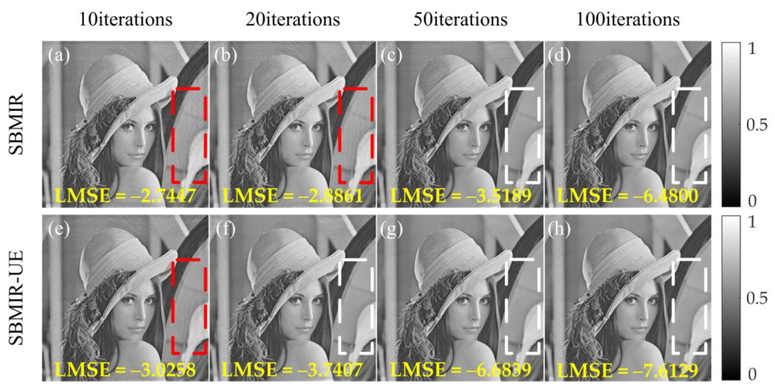
Except for the convergence speed, the convergence precision is also taken into account as an indicator for assessing the performance of the iterative method. Figure 3 shows the reconstructed normalized amplitude images after 10, 20, 50 and 100 iterations using SBMIR and SBMIR-UE, respectively. The logarithm of mean square error (LMSE) is adopted in order to quantitatively evaluate the quality of the reconstruction. In the figure, the part marked by the red rectangle indicates that the recovered result is significantly different from the ground truth, while the white rectangle means that the result is consistent with the target. These imperfect regions are gradually improved by both methods. However, the correction time of SBMIR is significantly longer than that of SBMIR-UE. SBMIR requires 50 iterations to eliminate errors. In contrast, SBMIR-UE can quickly reduce errors after 20 iterations, only because this method provides relatively rich intensity variation. It can be seen that the LMSE of SBMIR-UE is smaller than that of the traditional SBMIR under the same iteration times. What is more, the LMSE value at the 10th iteration of SBMIR-UE is −3.0258, which is smaller than the LMSE value of −2.8861 at the 20th iteration using the traditional method. These results prove that the proposed algorithm possesses superior recovery accuracy and convergence speed.

4. Experiment

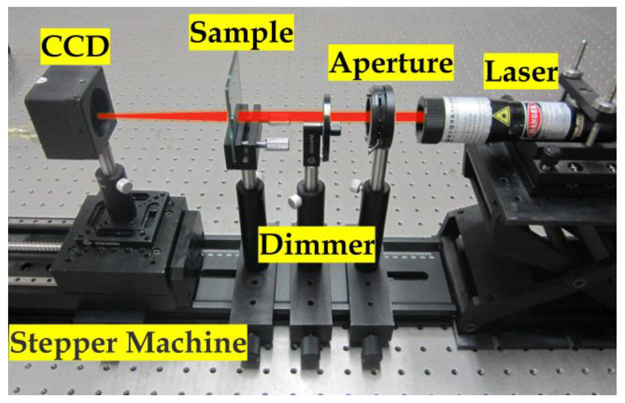
In order to further verify our method, the experiments were performed. Figure 4 shows the experimental setup. The working wavelength of the laser beam was 650 nm. The laser beam was adjusted by the aperture and dimmer and then illuminated the sample vertically. The CCD camera with a pixel size of 7.4 μm and resolution of 4896 × 3248 was fixed on the linear translation stage to capture diffraction patterns downstream of the sample. Firstly, the amplitude-type resolution plate was selected as the test sample. The initial distance was z₀ = 40 mm. The number of measurement planes was 6. The interval space of the adjacent plane of the conventional SBMIR was Δz = 10 mm. In the SBMIR-UE, plane interval spaces were set as follows: Δz₁ = 18 mm, Δz₂ = 14 mm, Δz₃ = 10 mm, Δz₄ = 6 mm, Δz₅ = 2 mm, and d = 4 mm.

To ensure the consistency of background noise and inclination error with the two methods, we continuously moved the CCD camera to 10 different positions to record the diffraction patterns (the two approaches share the same initial plane and final plane), as shown in Figure 5. The tilted illumination effect was corrected by the cross-correlation calibration and the Fourier-based strategy [35,36] before the iterative calculation. In the experiment, the incident light was not completely perpendicular to the CCD screen. According to the relative shifts in the diffraction images, we can calculate the tilt angle of the incident light by cross-correlation calibration. These patterns, deviating from the original center due to oblique illumination, can be aligned by Fourier frequency shift using the calculated angles. More detailed information can be found in the literature [35,36].

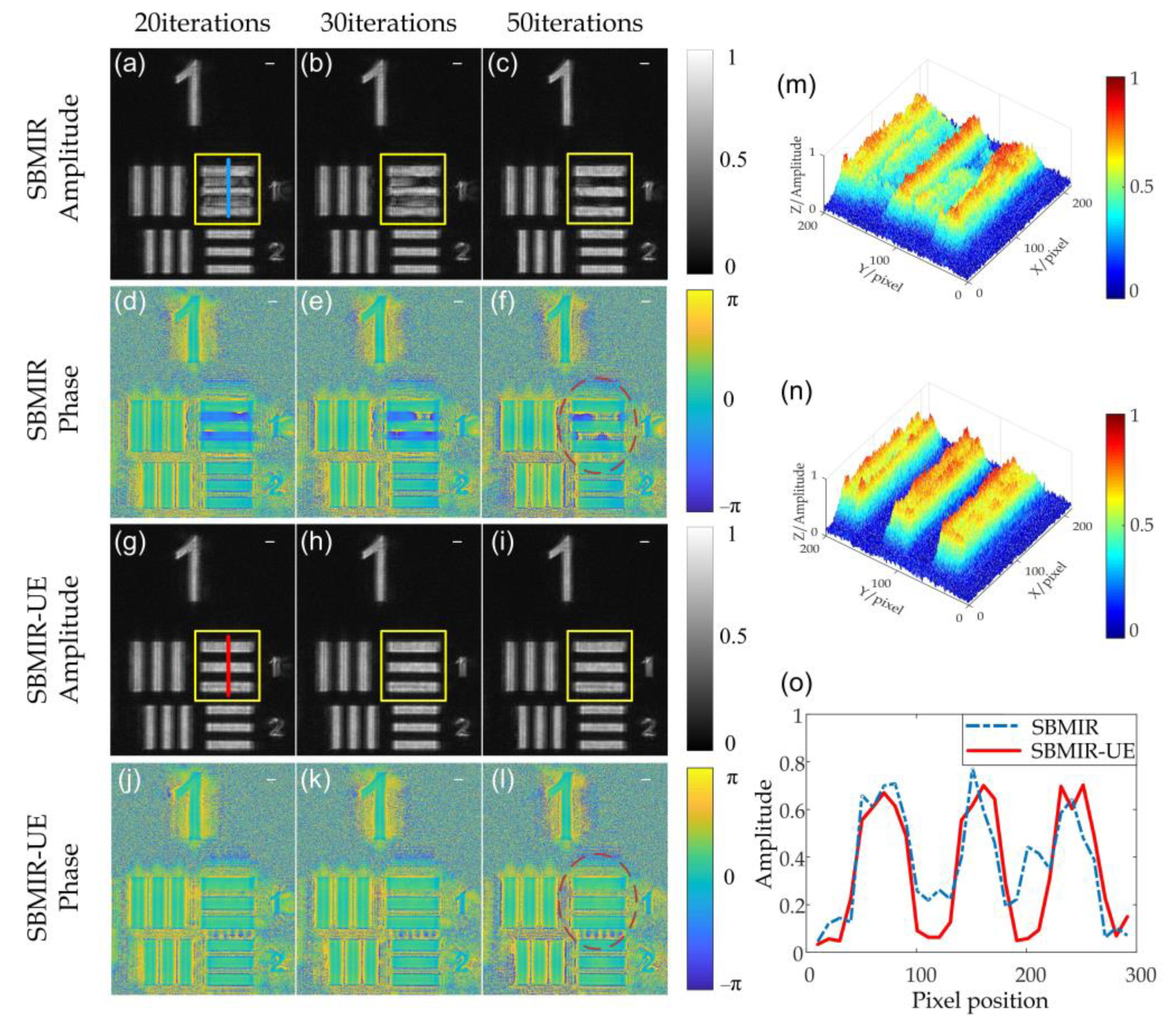
Figure 6 shows the reconstructed results. Apparently, some distinct obscure areas exist in each iteration result of SBMIR, as shown in Figure 6a–c. With increasing iteration times, the vague part is slowly corrected. However, in the improved method, SBMIR-UE eliminates the ambiguity at the beginning of the 20^th iteration. Moreover, SBMIR requires 60 iterations to eliminate the errors (image not shown here). The difference between the two algorithms can also be observed in the phase recovery results. In the proposed method, the phase distribution remains uniform for 20, 30 and 50 iterations, while in the traditional method, the circled recovered phases after 50 iterations (see Figure 6f) are inhomogeneous. We extract the data marked by yellow squares, as shown in Figure 6a,g, after 20 iterations and make a three-dimensional comparison in Figure 6m,n. It can be seen that the reconstruction results of the improved method have a high imaging contrast. In addition, the data captured from blue and red lines in Figure 6a,g are plotted in Figure 6o, which shows that the enhanced approach yields robust reconstructions and requires fewer iterations.

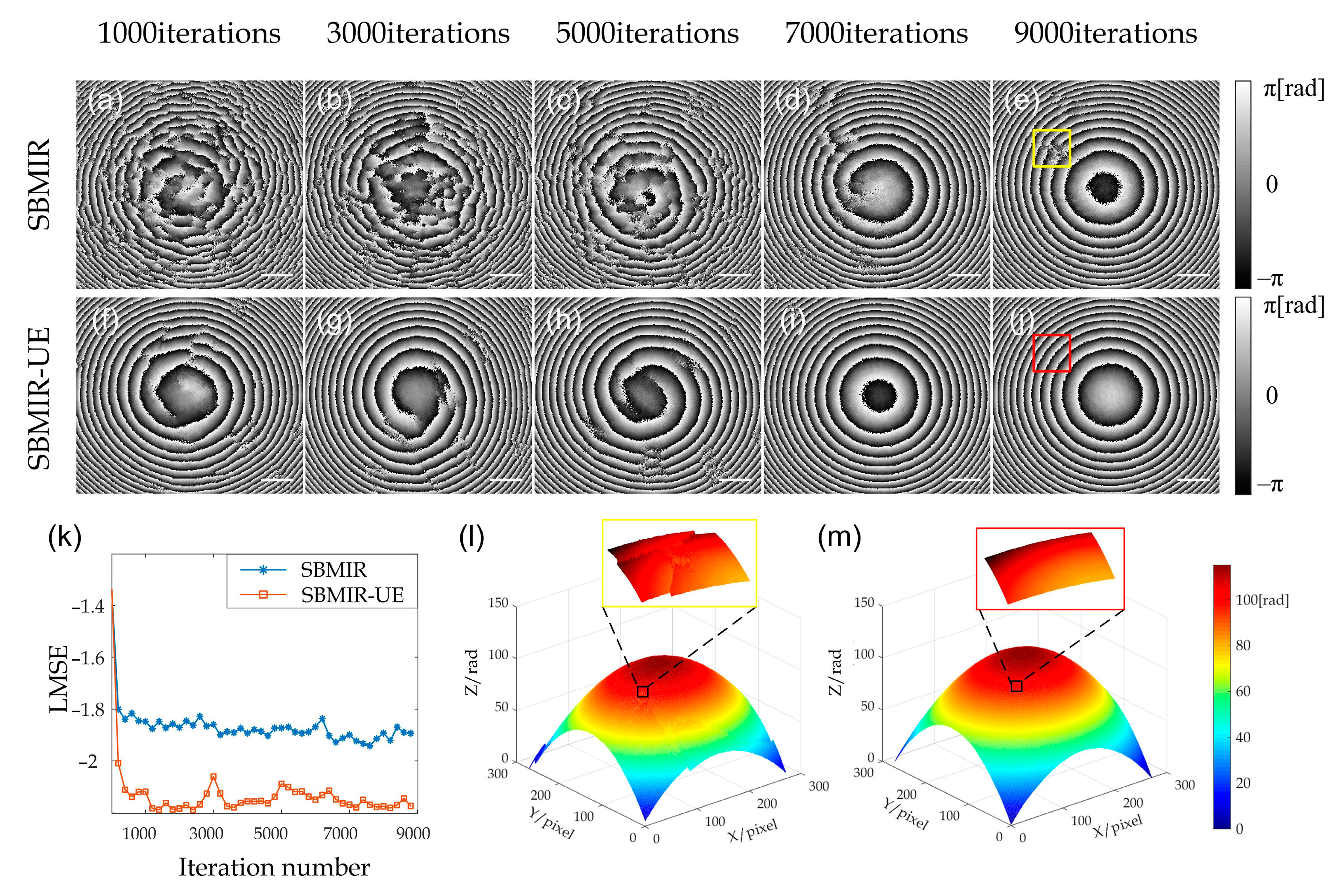
Secondly, a lens with a focal length of 8 cm was used as the phase-type sample with the following parameters: the initial distance was z₀ = 45 mm, the number of intensity planes was 6. The plane interval space of SBMIR was Δz = 30 mm, while the interval space in the SBMIR-UE was set as follows: Δz₁ = 58 mm, Δz₂ = 44 mm, Δz₃ = 30 mm, Δz₄ = 16 mm and Δz₅ = 2 mm, and the difference was d = 14 mm. Figure 7 shows the reconstructed results at different iterative times with the two different methods. It can be observed that the recovery process is prolonged in the conventional method. One obvious feature is that SBMIR reconstructs a similar result when running iteration times of up to 7000 and SBMIR-UE requires iteration times of 3000 only. It should be noted that the amplitude object converges within 100 iterations, while a phase object such as the lens requires thousands of iterative times. This is the reason that the phase object is relatively smooth, and the change in diffraction intensity is not significant enough. This results in a slow convergence rate. However, even in this case, our method is still faster than the traditional method.

In SBMIR, the quality of spherical fringes is not improved significantly with increasing iteration time. The accumulated errors in the propagation process will cause the final reconstruction to converge with the wrong results. The significant error of SBMIR after 9000 iteration times is marked by the yellow square in Figure 7e, and the red square marks the same position in SBMIR-UE, as shown in Figure 7j. We unwrap the final reconstruction phases, as shown in Figure 7l (SBMIR) and Figure 7m (SBMIR-UE). It is clarified that the surface of the phase reconstructed by the conventional method exhibits faults, while the reconstruction details achieved by the improved method are smooth. This phenomenon indicates that the proposed method avoids the unsatisfactory results caused by the lack of effective amplitude change in the uniform transmission process. Figure 7k shows the logarithm of mean square error (LMSE) between the measured and the reconstructed amplitude on the first plane using the two methods. This means that the proposed method has high recovery accuracy for the phase object.

5. Discussions

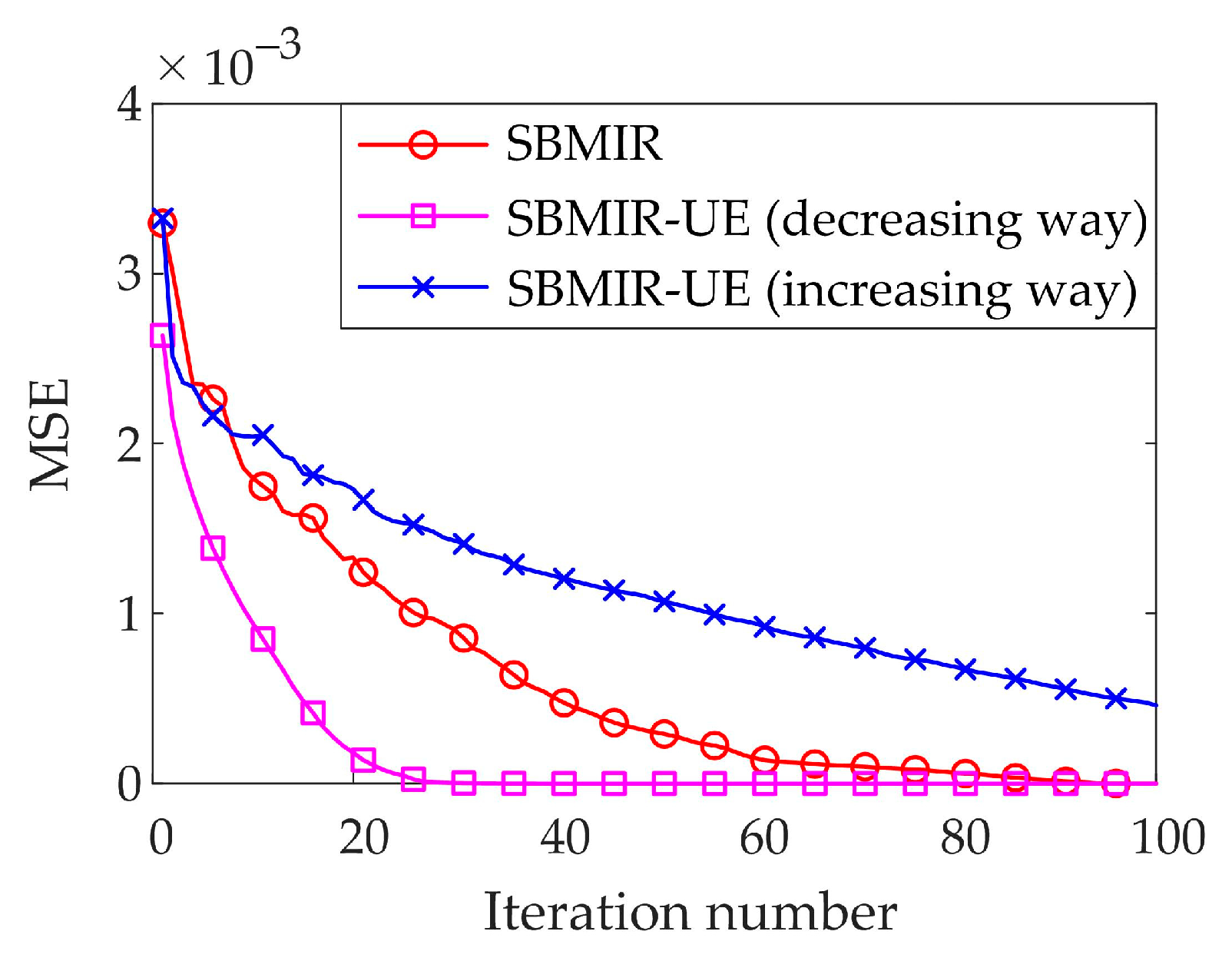
In this work, we demonstrate an unequal interval measurement method for the purpose of accelerating the convergence rate and enhancing the accuracy of SBMIR. It is worthwhile to mention that we choose a gradually decreasing interval distribution among the recordings rather than an increasing one. To confirm the effectiveness of the discussed strategies, we compare the performance of the two different methods in the simulation. Conveniently, we refer to the decreasing method and the increasing method hereinafter, and conventional SBMIR is cited as a reference. The parameters are consistent with the “simulation” part besides the parameter of “d”. In the decreasing spacing method, Δz₁ to Δz₄ are set to be 13.5, 9.5, 5.5, 1.5 mm, respectively, with d = 4 mm. For the increasing method, Δz₁ to Δz₄ are set to be 1.5, 5.5, 9.5, 13.5 mm, respectively, with d = 4 mm. The simulation results are shown in Figure 8. It is apparent that the decreasing method (purple line) converges faster than the increasing method (blue line). It can be explained that the closer the recorded patterns are to the sample, the greater the similarity among them will be. Thus, there will be the problem of convergence delay. Consequently, we finally choose the variation from large to small distance as our discussion method.

As a matter of fact, the unequal interval method has been proposed by T. Kozacki’s group in order to reduce the error of phase recovery [37,38]. However, there are still significant differences between their works and ours. Firstly, in terms of the algorithm, the technique in the literature uses the Transport of Intensity Equation (TIE) to reconstruct the phases, but we adopt the SBMIR based on the angular spectrum theory. Secondly, for the purpose of non-equidistant measurement, TIE-based phase retrieval aims at selecting a set of planes that can equalize the error contribution of all frequency bands. We hope to find a set of patterns where the cross-correlation coefficient gradually increases, so as to ensure both the convergence speed and the convergence precision. Thirdly, in the design of position parameters of experiments, the original TIE-based technique utilizes increasing spacing between records. Meanwhile, both a positive and negative reference plane are used. The spacing of the planes is equally decreased in our method. The reason for abandoning the increasing spacing is that the gradually increasing distance will lead to the relatively strong similarity of the several planes recorded at the beginning and further cause the delay of convergence. Fourthly, TIE has a high requirement (down to micron scale) for the interval spacing of adjacent planes. In our cases, we allow the position of the plane to be measured at the level of millimeters or even centimeters. The TIE-based approach is not applicable to our iterative algorithm or the real experiment. As for the criterion for distance selection, the key issue in TIE-based phase retrieval techniques is the optimum estimation of the axial intensity derivative. The calculation of the intensity derivative implies a priori knowledge of several parameters, such as signal-to-noise ratio, number of planes and plane separation. The TIE-based algorithm takes all of this into account in selecting the optimized distance [39]. In SBMIR, the key issue for successful iterative phase retrieval is the significant intensity variations in adjacent propagation planes, while using the lowest number of measurements. Therefore, we take the intensity change as our distance selection criterion and propose the cross-correlation coefficient to represent the intensity change. Our method may not be original in terms of unequal interval measurement. However, our method is the first to propose the use of the cross-correlation coefficient to resolve the optimal distance. The method of interval setting is also different from the previously reported strategy of exponential interval distribution, which is a simple arithmetic sequence distribution.

6. Summary

In summary, an enhanced multi-distance phase retrieval method is proposed. The difference between the conventional method of SBMIR and our proposed SBMIR-UE is that the interval space between measurement planes is varied from long distance to short distance. This method can effectively improve the convergence speed and enhance the quality of reconstruction, especially since it does not require additional modulation equipment, complex algorithms or strict constraints. This non-equidistant principle is an effective strategy for robust phase recovery and can be expected to be used in the techniques of rapid multi-distance phase recovery.