Physical and Methodological Perspectives on the Optical Properties of Biological Samples: A Review

 ,
, 
Abstract
:1. Introduction
1.1. Applications and Optical Spectra in Biological Samples
1.2. Basic Principles of Microscopy and Optical Properties of Tissues
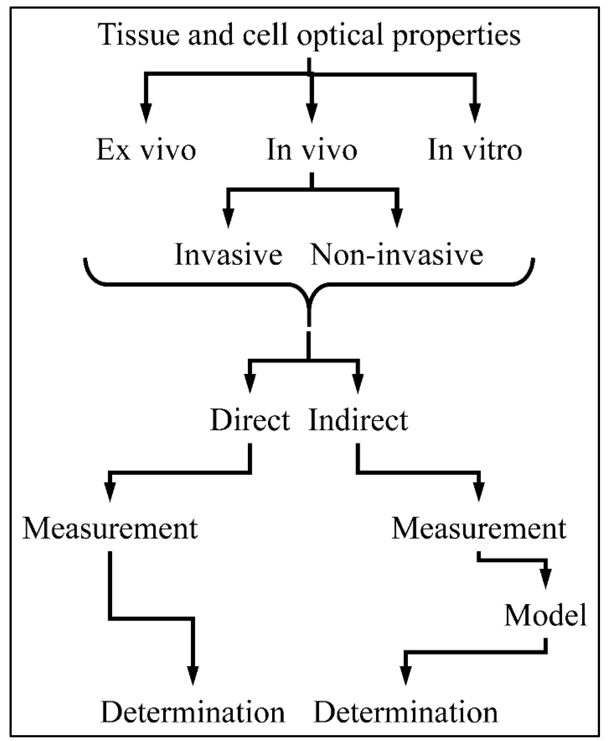
1.3. Measuring Tissue’s Optical Properties
2. Theoretical Concepts for Optical Properties in Biological Studies
2.1. Scattering
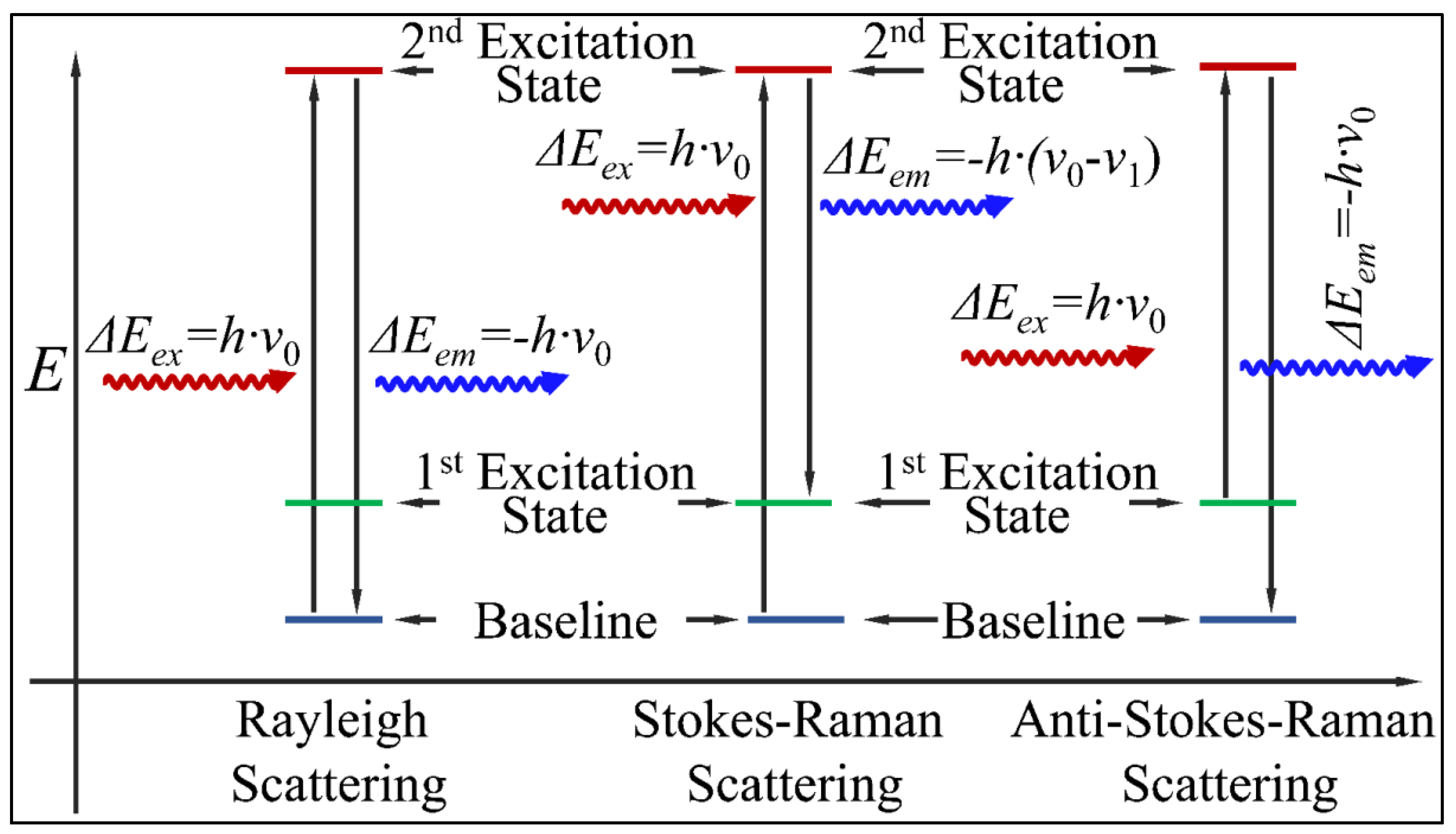
2.1.1. Rayleigh Scattering
2.1.2. Stokes–Raman and Anti-Stokes–Raman Scattering
2.1.3. Scattering Coefficient
2.1.4. Reduced Scattering Coefficient
2.1.5. Scattering and Anisotropy
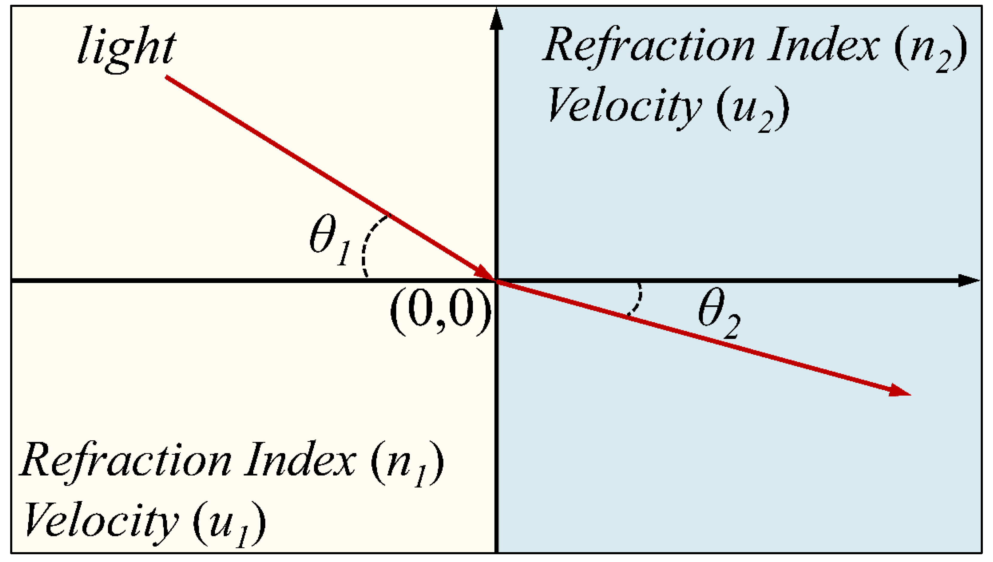
2.2. Refraction
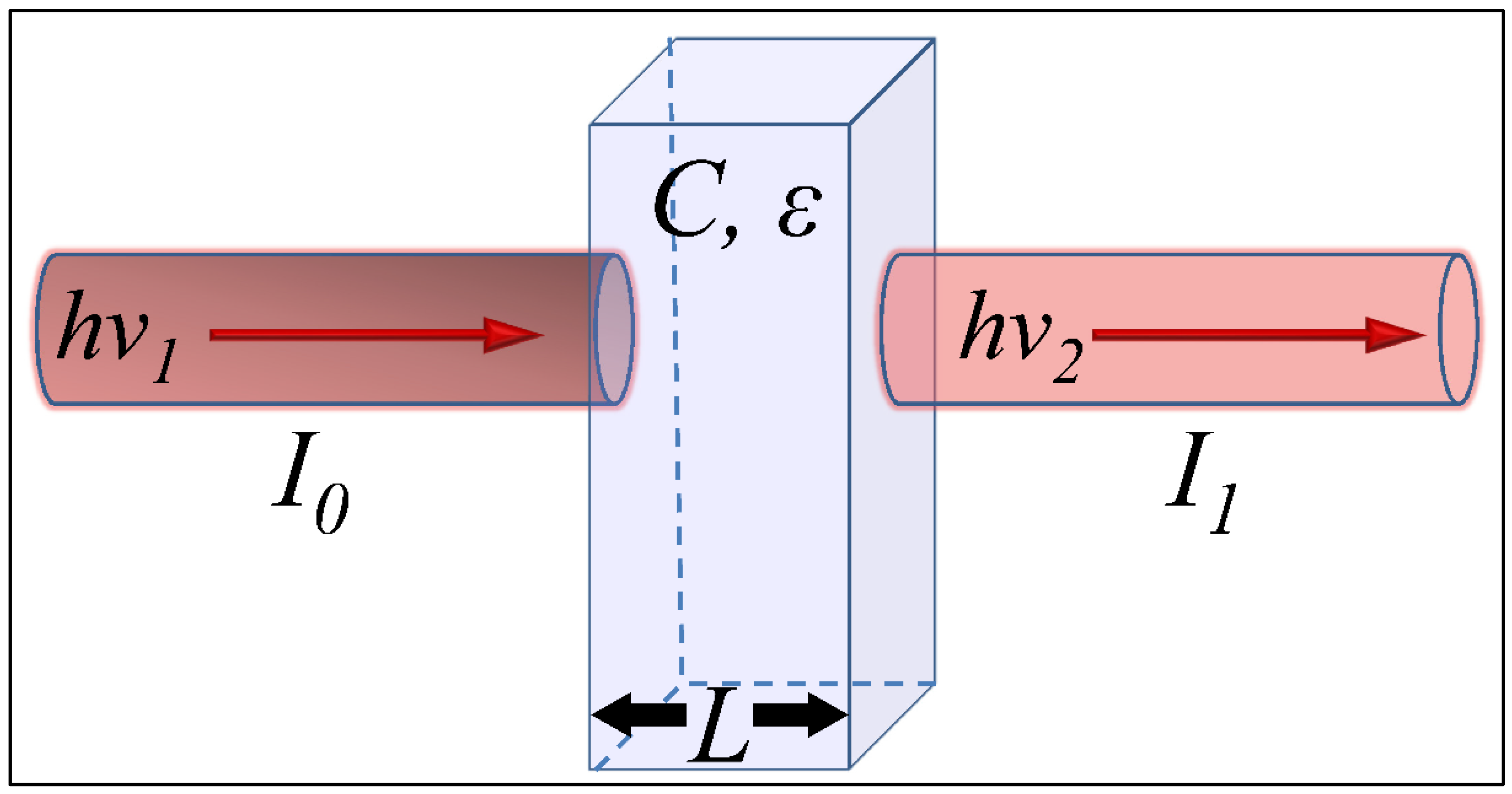
2.3. Absorption
2.3.1. Definition and Mathematical Terms
2.3.2. Water
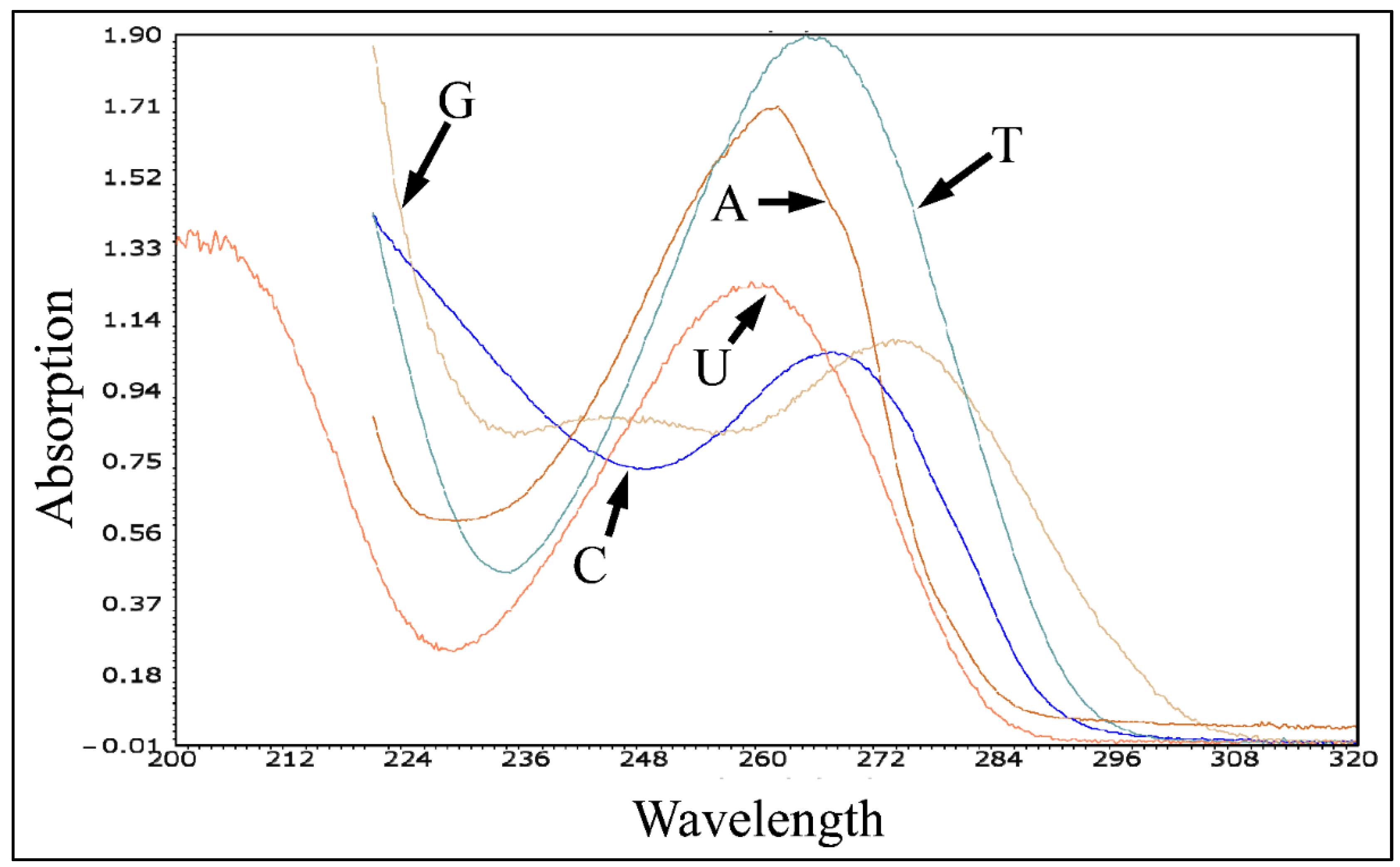
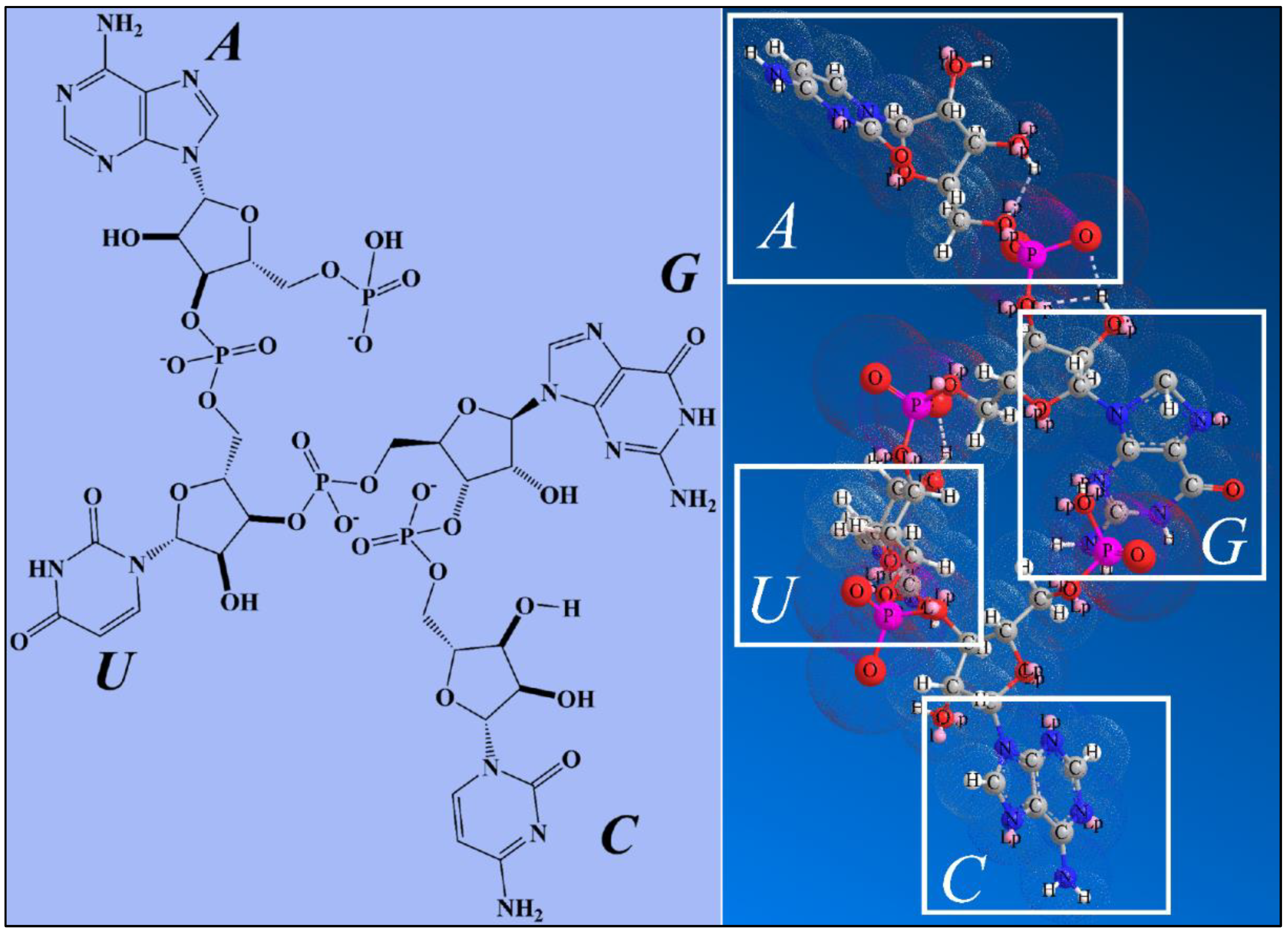
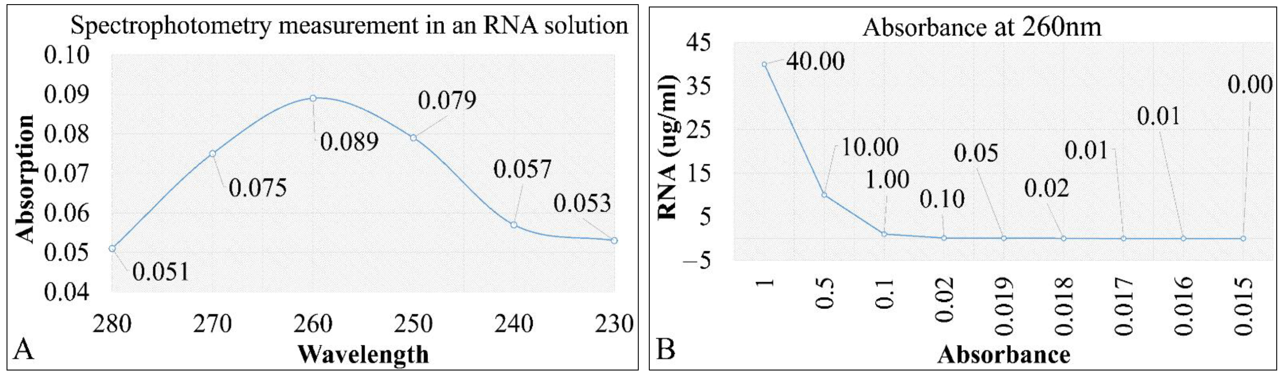
2.3.3. Nucleotides
2.3.4. Hemoglobin and Blood
2.3.5. Melanosomes, Melanocytes and Melanin
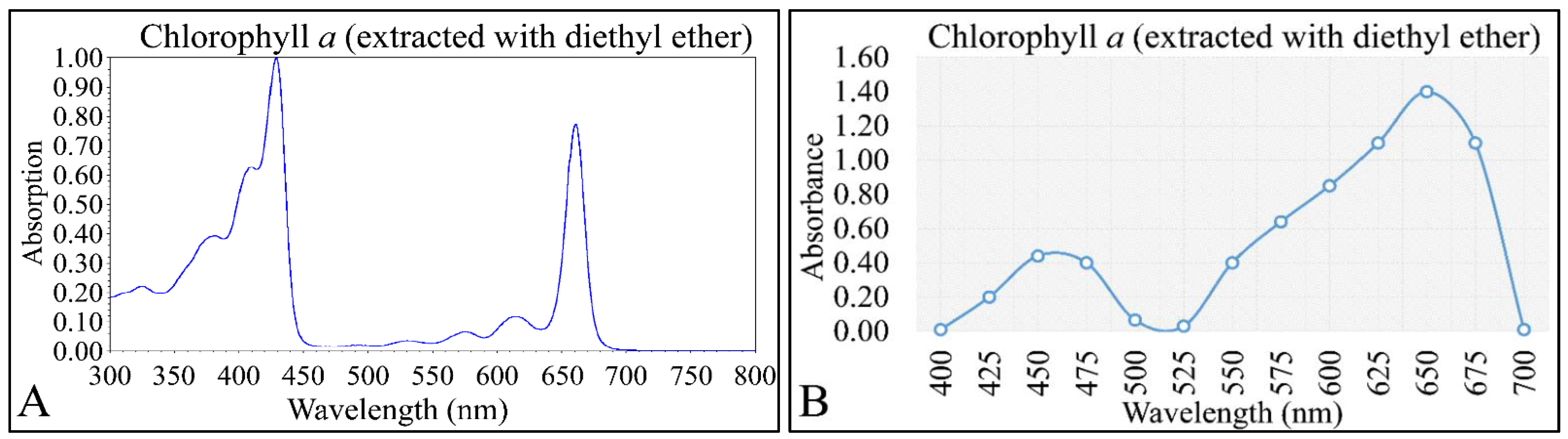
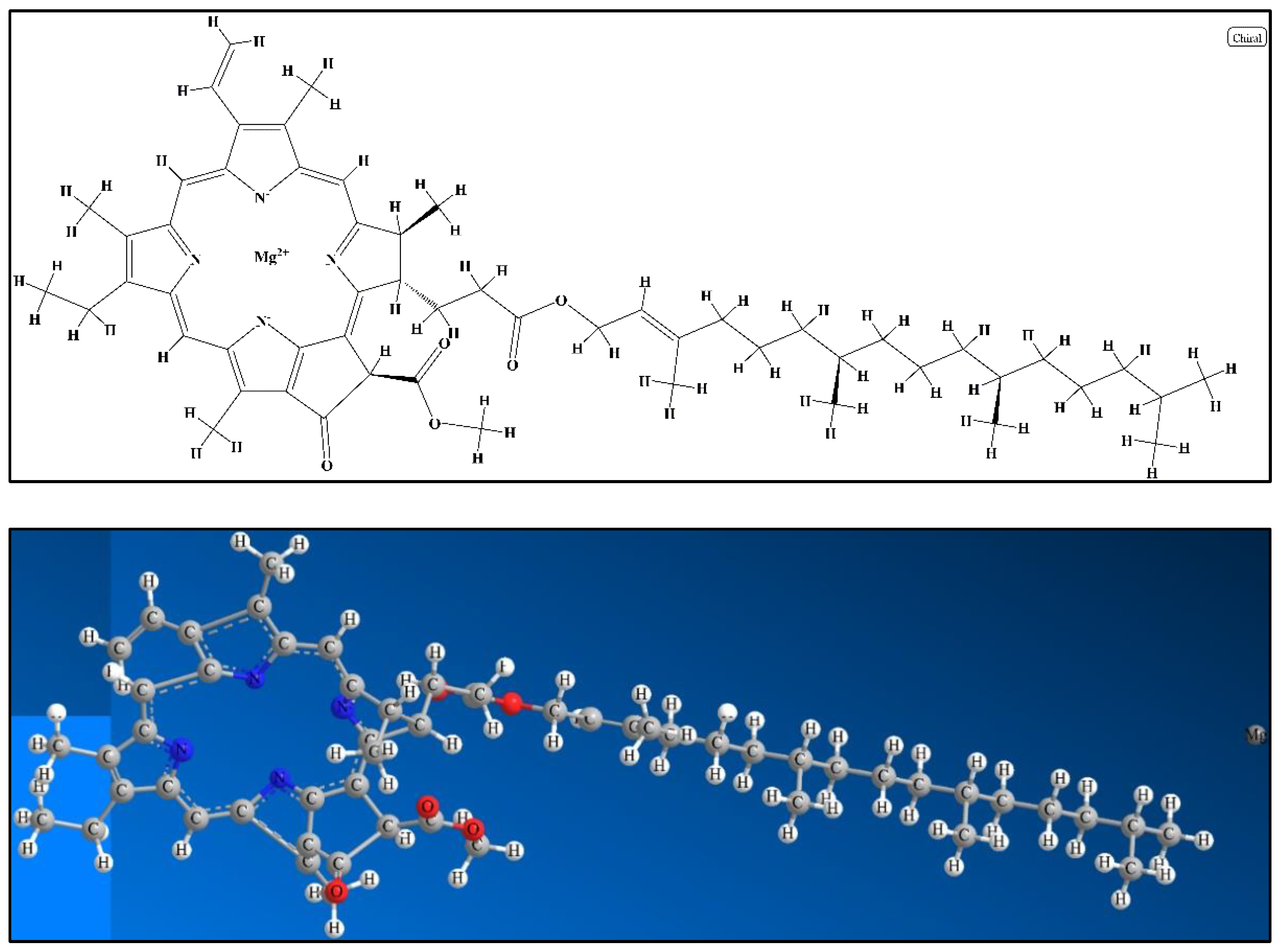
2.3.6. Chlorophyll
2.3.7. Adipose Tissue
2.4. Optical Properties in Non-Spherical Particles: The Case of Real Life
3. Methods for Studying the Optical Properties of Tissues: The Case of Monte Carlo Simulations
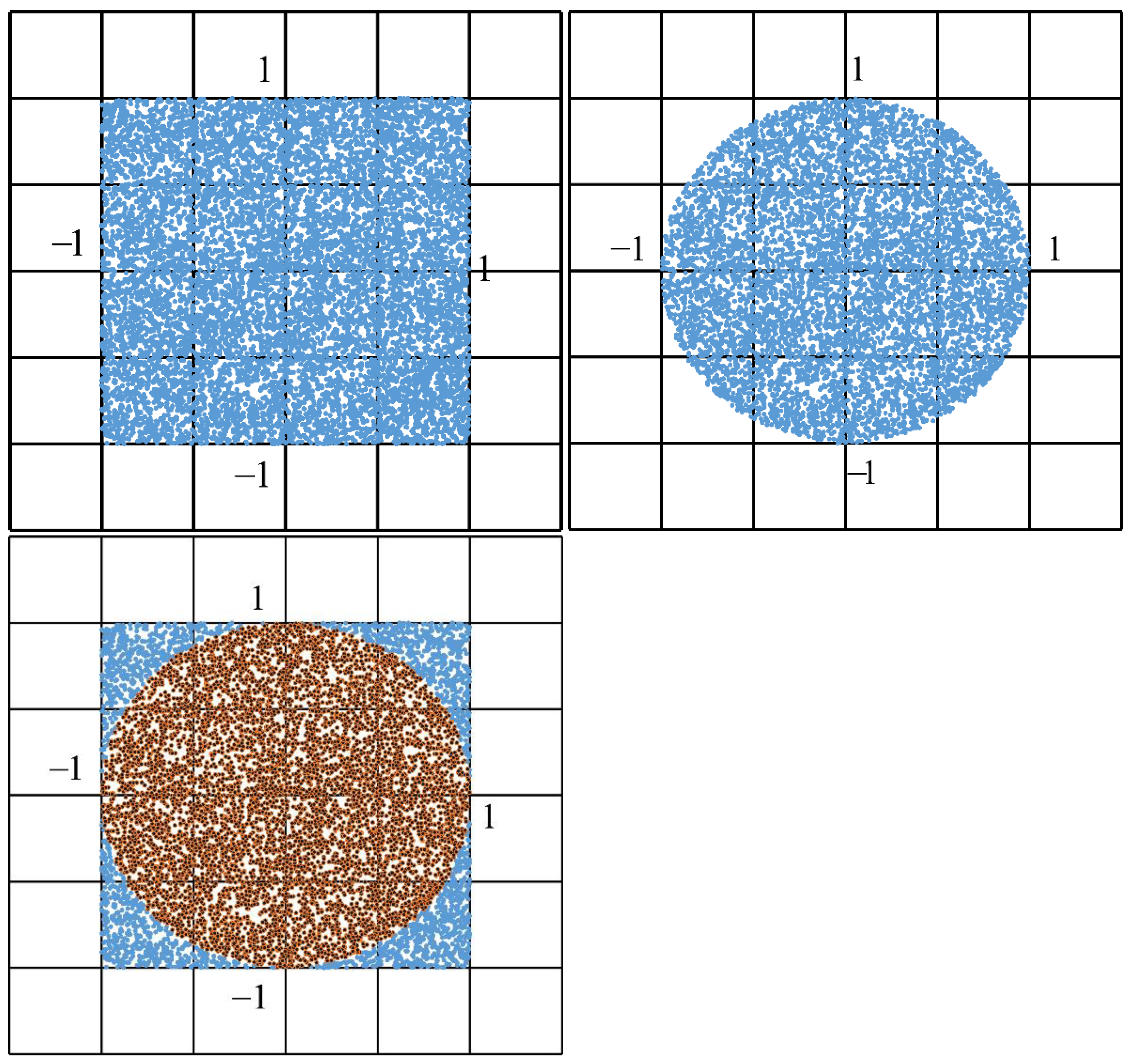
3.1. The Monte Carlo Simulation: A Short History
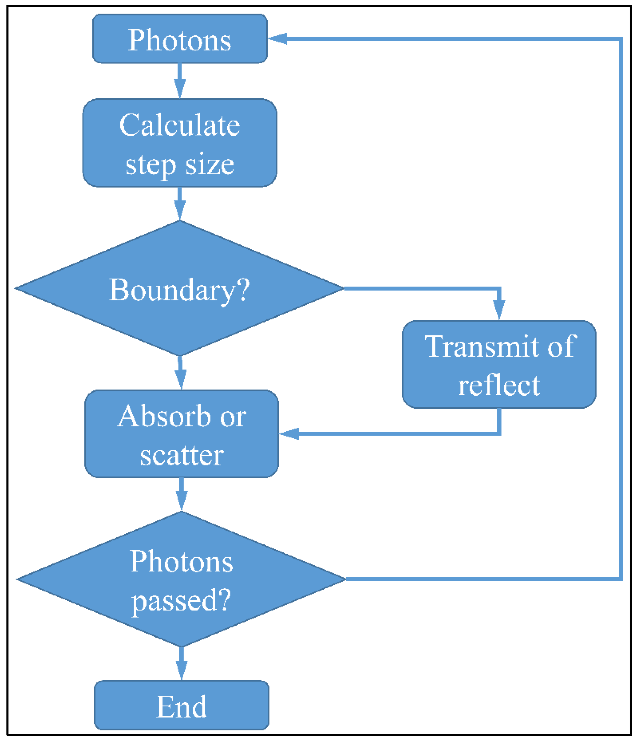
3.2. Numerical Solution of the Monte Carlo Method
4. Conclusions
Author Contributions
Funding

Institutional Review Board Statement
Informed Consent Statement
Data Availability Statement
Conflicts of Interest
References
- Abbas, M.; Ali, M.; Shah, S.K.; D’Amico, F.; Postorino, P.; Mangialardo, S.; Cestelli Guidi, M.; Cricenti, A.; Gunnella, R. Control of structural, electronic, and optical properties of eumelanin films by electrospray deposition. J. Phys. Chem. B 2011, 115, 11199–11207. [Google Scholar] [CrossRef]
- Gutierrez-Juarez, G.; Gupta, S.K.; Weight, R.M.; Polo-Parada, L.; Papagiorgio, C.; Bunch, J.D.; Viator, J.A. Optical photoacoustic detection of circulating melanoma cells in vitro. Int. J. Thermophys. 2010, 31, 784–792. [Google Scholar] [CrossRef] [PubMed] [Green Version]
- Krohn, J.; Svenmarker, P.; Xu, C.T.; Mork, S.J.; Andersson-Engels, S. Transscleral optical spectroscopy of uveal melanoma in enucleated human eyes. Investig. Ophthalmol. Vis. Sci. 2012, 53, 5379–5385. [Google Scholar] [CrossRef] [Green Version]
- Olsen, J.; Themstrup, L.; Jemec, G.B. Optical coherence tomography in dermatology. G. Ital. Dermatol. E Venereol. Organo Uff. Soc. Ital. Dermatol. E Sifilogr. 2015, 150, 603–615. [Google Scholar]
- Omar, M.; Schwarz, M.; Soliman, D.; Symvoulidis, P.; Ntziachristos, V. Pushing the optical imaging limits of cancer with multi-frequency-band raster-scan optoacoustic mesoscopy (rsom). Neoplasia 2015, 17, 208–214. [Google Scholar] [CrossRef] [Green Version]
- Tseng, S.H.; Hou, M.F. Analysis of a diffusion-model-based approach for efficient quantification of superficial tissue properties. Opt. Lett. 2010, 35, 3739–3741. [Google Scholar] [CrossRef] [PubMed]
- Wahab, R.; Dwivedi, S.; Umar, A.; Singh, S.; Hwang, I.H.; Shin, H.S.; Musarrat, J.; Al-Khedhairy, A.A.; Kim, Y.S. Zno nanoparticles induce oxidative stress in cloudman s91 melanoma cancer cells. J. Biomed. Nanotechnol. 2013, 9, 441–449. [Google Scholar] [CrossRef]
- Wang, H.; Yi, J.; Mukherjee, S.; Banerjee, P.; Zhou, S. Magnetic/nir-thermally responsive hybrid nanogels for optical temperature sensing, tumor cell imaging and triggered drug release. Nanoscale 2014, 6, 13001–13011. [Google Scholar] [CrossRef]
- Deb, P.; Sharma, M.C.; Tripathi, M.; Sarat Chandra, P.; Gupta, A.; Sarkar, C. Expression of cd34 as a novel marker for glioneuronal lesions associated with chronic intractable epilepsy. Neuropathol. Appl. Neurobiol. 2006, 32, 461–468. [Google Scholar] [CrossRef] [PubMed]
- Stankovic, T.; Marston, E. Molecular mechanisms involved in chemoresistance in paediatric acute lymphoblastic leukaemia. Srp. Arh. Za Celok. Lek. 2008, 136, 187–192. [Google Scholar] [CrossRef]
- Weller, M.; Berger, H.; Hartmann, C.; Schramm, J.; Westphal, M.; Simon, M.; Goldbrunner, R.; Krex, D.; Steinbach, J.P.; Ostertag, C.B.; et al. Combined 1p/19q loss in oligodendroglial tumors: Predictive or prognostic biomarker? Clin. Cancer Res. 2007, 13, 6933–6937. [Google Scholar] [CrossRef] [Green Version]
- Moolgavkar, S.H.; Knudson, A.G., Jr. Mutation and cancer: A model for human carcinogenesis. J. Natl. Cancer Inst. 1981, 66, 1037–1052. [Google Scholar] [CrossRef] [PubMed]
- Belda-Iniesta, C.; de Castro Carpeno, J.; Casado Saenz, E.; Cejas Guerrero, P.; Perona, R.; Gonzalez Baron, M. Molecular biology of malignant gliomas. Clin. Transl. Oncol. 2006, 8, 635–641. [Google Scholar] [CrossRef] [PubMed]
- Rutkowski, S. Current treatment approaches to early childhood medulloblastoma. Expert Rev. Neurother. 2006, 6, 1211–1221. [Google Scholar] [CrossRef]
- Sanson, M.; Thillet, J.; Hoang-Xuan, K. Molecular changes in gliomas. Curr. Opin. Oncol. 2004, 16, 607–613. [Google Scholar] [CrossRef] [PubMed]
- Assayag, O.; Antoine, M.; Sigal-Zafrani, B.; Riben, M.; Harms, F.; Burcheri, A.; Grieve, K.; Dalimier, E.; Le Conte de Poly, B.; Boccara, C. Large field, high resolution full-field optical coherence tomography: A pre-clinical study of human breast tissue and cancer assessment. Technol. Cancer Res. Treat. 2014, 13, 455–468. [Google Scholar] [CrossRef] [PubMed] [Green Version]
- Diaconu, I.; Cristea, C.; Harceaga, V.; Marrazza, G.; Berindan-Neagoe, I.; Sandulescu, R. Electrochemical immunosensors in breast and ovarian cancer. Clin. Chim. Acta Int. J. Clin. Chem. 2013, 425, 128–138. [Google Scholar] [CrossRef]
- Hayashi, K.; Tamari, K.; Ishii, H.; Konno, M.; Nishida, N.; Kawamoto, K.; Koseki, J.; Fukusumi, T.; Kano, Y.; Nishikawa, S.; et al. Visualization and characterization of cancer stem-like cells in cervical cancer. Int. J. Oncol. 2014, 45, 2468–2474. [Google Scholar] [CrossRef] [Green Version]
- Herranz, M.; Ruibal, A. Optical imaging in breast cancer diagnosis: The next evolution. J. Oncol. 2012, 2012, 863747. [Google Scholar] [CrossRef] [Green Version]
- Kennedy, B.F.; McLaughlin, R.A.; Kennedy, K.M.; Chin, L.; Wijesinghe, P.; Curatolo, A.; Tien, A.; Ronald, M.; Latham, B.; Saunders, C.M.; et al. Investigation of optical coherence microelastography as a method to visualize cancers in human breast tissue. Cancer Res. 2015, 75, 3236–3245. [Google Scholar] [CrossRef] [Green Version]
- Li, B.; Cheng, Y.; Liu, J.; Yi, C.; Brown, A.S.; Yuan, H.; Vo-Dinh, T.; Fischer, M.C.; Warren, W.S. Direct optical imaging of graphene in vitro by nonlinear femtosecond laser spectral reshaping. Nano Lett. 2012, 12, 5936–5940. [Google Scholar] [CrossRef] [PubMed] [Green Version]
- Vardaki, M.Z.; Gardner, B.; Stone, N.; Matousek, P. Studying the distribution of deep raman spectroscopy signals using liquid tissue phantoms with varying optical properties. Analyst 2015, 140, 5112–5119. [Google Scholar] [CrossRef] [PubMed] [Green Version]
- Wang, L.W.; Peng, C.W.; Chen, C.; Li, Y. Quantum dots-based tissue and in vivo imaging in breast cancer researches: Current status and future perspectives. Breast Cancer Res. Treat. 2015, 151, 7–17. [Google Scholar] [CrossRef] [Green Version]
- Yan, X.; Zhou, Y.; Liu, S. Optical imaging of tumors with copper-labeled rhodamine derivatives by targeting mitochondria. Theranostics 2012, 2, 988–998. [Google Scholar] [CrossRef] [PubMed] [Green Version]
- Shai, R.M.; Reichardt, J.K.; Chen, T.C. Pharmacogenomics of brain cancer and personalized medicine in malignant gliomas. Future Oncol. 2008, 4, 525–534. [Google Scholar] [CrossRef]
- Allison, R.R. Photodynamic therapy: Oncologic horizons. Future Oncol. 2014, 10, 123–124. [Google Scholar] [CrossRef]
- Bechet, D.; Mordon, S.R.; Guillemin, F.; Barberi-Heyob, M.A. Photodynamic therapy of malignant brain tumours: A complementary approach to conventional therapies. Cancer Treat. Rev. 2014, 40, 229–241. [Google Scholar] [CrossRef]
- Miki, Y.; Akimoto, J.; Yokoyama, S.; Homma, T.; Tsutsumi, M.; Haraoka, J.; Hirano, K.; Beppu, M. Photodynamic therapy in combination with talaporfin sodium induces mitochondrial apoptotic cell death accompanied with necrosis in glioma cells. Biol. Pharm. Bull. 2013, 36, 215–221. [Google Scholar] [CrossRef] [Green Version]
- Smirnova, Z.S.; Ermakova, K.V.; Kubasova, I.Y.; Borisova, L.M.; Kiselyova, M.P.; Oborotova, N.A.; Meerovich, G.A.; Luk’yanets, E.A. Experimental study of combined therapy for malignant glioma. Bull. Exp. Biol. Med. 2014, 156, 480–482. [Google Scholar] [CrossRef]
- Sun, W.; Kajimoto, Y.; Inoue, H.; Miyatake, S.; Ishikawa, T.; Kuroiwa, T. Gefitinib enhances the efficacy of photodynamic therapy using 5-aminolevulinic acid in malignant brain tumor cells. Photodiagn. Photodyn. Ther. 2013, 10, 42–50. [Google Scholar] [CrossRef]
- Tzerkovsky, D.A.; Osharin, V.V.; Istomin, Y.P.; Alexandrova, E.N.; Vozmitel, M.A. Fluorescent diagnosis and photodynamic therapy for c6 glioma in combination with antiangiogenic therapy in subcutaneous and intracranial tumor models. Exp. Oncol. 2014, 36, 85–89. [Google Scholar]
- Conteduca, D.; Brunetti, G.; Dell’Olio, F.; Armenise, M.N.; Krauss, T.F.; Ciminelli, C. Monitoring of individual bacteria using electro-photonic traps. Biomed. Opt. Express 2019, 10, 3463–3471. [Google Scholar] [CrossRef] [PubMed]
- Zhou, H.; Yang, D.; Ivleva, N.P.; Mircescu, N.E.; Schubert, S.; Niessner, R.; Wieser, A.; Haisch, C. Label-free in situ discrimination of live and dead bacteria by surface-enhanced raman scattering. Anal. Chem. 2015, 87, 6553–6561. [Google Scholar] [CrossRef]
- Lopez, D.; Vlamakis, H.; Kolter, R. Biofilms. Cold Spring Harb. Perspect. Biol. 2010, 2, a000398. [Google Scholar] [CrossRef]
- Hall-Stoodley, L.; Costerton, J.W.; Stoodley, P. Bacterial biofilms: From the natural environment to infectious diseases. Nat. Rev. Microbiol. 2004, 2, 95–108. [Google Scholar] [CrossRef] [PubMed]
- Brunetti, G.; Conteduca, D.; Armenise, M.N.; Ciminelli, C. Novel micro-nano optoelectronic biosensor for label-free real-time biofilm monitoring. Biosensors 2021, 11, 361. [Google Scholar] [CrossRef]
- Petrovszki, D.; Valkai, S.; Gora, E.; Tanner, M.; Banyai, A.; Furjes, P.; Der, A. An integrated electro-optical biosensor system for rapid, low-cost detection of bacteria. Microelectron. Eng. 2021, 239, 111523. [Google Scholar] [CrossRef]
- Yoo, D.; Gurunatha, K.L.; Choi, H.K.; Mohr, D.A.; Ertsgaard, C.T.; Gordon, R.; Oh, S.H. Low-power optical trapping of nanoparticles and proteins with resonant coaxial nanoaperture using 10 nm gap. Nano Lett. 2018, 18, 3637–3642. [Google Scholar] [CrossRef]
- Conteduca, D.; Brunetti, G.; Pitruzzello, G.; Tragni, F.; Dholakia, K.; Krauss, T.F.; Ciminelli, C. Exploring the limit of multiplexed near-field optical trapping. Acs Photonics 2021, 8, 2060–2066. [Google Scholar] [CrossRef]
- Jacques, S.L. Optical properties of biological tissues: A review. Phys. Med. Biol. 2013, 58, R37–R61. [Google Scholar] [CrossRef]
- Jacques, S.L.; Pogue, B.W. Tutorial on diffuse light transport. J. Biomed. Opt. 2008, 13, 041302. [Google Scholar] [CrossRef] [PubMed] [Green Version]
- Sandell, J.L.; Zhu, T.C. A review of in-vivo optical properties of human tissues and its impact on pdt. J. Biophotonics 2011, 4, 773–787. [Google Scholar] [CrossRef] [Green Version]
- Zhu, T.C.; Liang, X.; Chang, C.; Sandell, J.; Finlay, J.C.; Dimofte, A.; Rodrigeus, C.; Cengel, K.; Friedberg, J.; Glatstein, E.; et al. An ir navigation system for real-time treatment guidance of pleural pdt. In Proceedings of the Optical Methods for Tumor Treatment and Detection: Mechanisms and Techniques in Photodynamic Therapy XX, San Francisco, CA, USA, 22–27 January 2011; Volume 7886. [Google Scholar]
- Eisel, M.; Strobl, S.; Pongratz, T.; Stepp, H.; Ruhm, A.; Sroka, R. Investigation of optical properties of dissected and homogenized biological tissue. J. Biomed. Opt. 2018, 23, 1–9. [Google Scholar] [CrossRef]
- Wilson, B.C. Measurement of tissue optical properties: Methods and theories. In Optical-Thermal Response of Laser-Irradiated Tissue; Welch, A.J., Van Gemert, M.J.C., Eds.; Springer: Boston, MA, USA, 1995; pp. 233–303. [Google Scholar]
- Van de Hulst, H.C.; Twersky, V. Light scattering by small particles. Phys. Today 1957, 10, 28–30. [Google Scholar] [CrossRef]
- Prahl, S. Optical property measurements using the inverse adding-doubling program. Or. Med Laser Cent. St. Vincent Hosp. 1999, 9205, 1–53. [Google Scholar]
- Chen, B.; Stamnes, K.; Stamnes, J.J. Validity of the diffusion approximation in bio-optical imaging. Appl. Opt. 2001, 40, 6356–6366. [Google Scholar] [CrossRef]
- Mie, G. Beiträge zur optik trüber medien, speziell kolloidaler metallösungen. Ann. Phys. 1908, 330, 377–445. [Google Scholar] [CrossRef]
- Yi, J.; Backman, V. Imaging a full set of optical scattering properties of biological tissue by inverse spectroscopic optical coherence tomography. Opt. Lett. 2012, 37, 4443–4445. [Google Scholar] [CrossRef] [Green Version]
- Einstein, A. Méthode pour la détermination de valeurs statistiques d’observations concernant des grandeurs soumises à des fluctuations irrégulières. Arch. Des Sci. 1914, 37, 254. [Google Scholar]
- Wiener, N. Generalized harmonic analysis. Acta Math. 1930, 55, 117–258. [Google Scholar] [CrossRef]
- Parseval, M.-A. Mémoire sur les séries et sur l’intégration complète d’une équation aux différences partielles linéaires du second ordre, à coefficients constants. Mém. Prés. Par Divers Savants Acad. Des Sci. Paris 1806, 1, 638–648. [Google Scholar]
- Fung, A.A.; Shi, L. Mammalian cell and tissue imaging using raman and coherent raman microscopy. Wiley Interdiscip. Rev. Syst. Biol. Med. 2020, 12, e1501. [Google Scholar] [CrossRef] [PubMed]
- Bevilacqua, F.; Berger, A.J.; Cerussi, A.E.; Jakubowski, D.; Tromberg, B.J. Broadband absorption spectroscopy in turbid media by combined frequency-domain and steady-state methods. Appl. Opt. 2000, 39, 6498–6507. [Google Scholar] [CrossRef] [Green Version]
- Cerussi, A.E.; Berger, A.J.; Bevilacqua, F.; Shah, N.; Jakubowski, D.; Butler, J.; Holcombe, R.F.; Tromberg, B.J. Sources of absorption and scattering contrast for near-infrared optical mammography. Acad. Radiol. 2001, 8, 211–218. [Google Scholar] [CrossRef] [Green Version]
- Durduran, T.; Choe, R.; Culver, J.P.; Zubkov, L.; Holboke, M.J.; Giammarco, J.; Chance, B.; Yodh, A.G. Bulk optical properties of healthy female breast tissue. Phys. Med. Biol. 2002, 47, 2847–2861. [Google Scholar] [CrossRef] [PubMed] [Green Version]
- Firbank, M.; Hiraoka, M.; Essenpreis, M.; Delpy, D.T. Measurement of the optical properties of the skull in the wavelength range 650–950 nm. Phys. Med. Biol. 1993, 38, 503–510. [Google Scholar] [CrossRef] [PubMed]
- Gardner, C.M.; Jacques, S.L.; Welch, A.J. Light transport in tissue: Accurate expressions for one-dimensional fluence rate and escape function based upon monte carlo simulation. Lasers Surg. Med. 1996, 18, 129–138. [Google Scholar] [CrossRef]
- Parsa, P.; Jacques, S.L.; Nishioka, N.S. Optical properties of rat liver between 350 and 2200 nm. Appl. Opt. 1989, 28, 2325–2330. [Google Scholar] [CrossRef]
- Saidi, I.S.; Jacques, S.L.; Tittel, F.K. Mie and rayleigh modeling of visible-light scattering in neonatal skin. Appl. Opt. 1995, 34, 7410–7418. [Google Scholar] [CrossRef] [PubMed]
- Salomatina, E.; Jiang, B.; Novak, J.; Yaroslavsky, A.N. Optical properties of normal and cancerous human skin in the visible and near-infrared spectral range. J. Biomed. Opt. 2006, 11, 064026. [Google Scholar] [CrossRef]
- Svaasand, L.O.; Wyss, P.; Wyss, M.T.; Tadir, Y.; Tromberg, B.J.; Berns, M.W. Dosimetry model for photodynamic therapy with topically administered photosensitizers. Lasers Surg. Med. 1996, 18, 139–149. [Google Scholar] [CrossRef]
- Taroni, P.; Danesini, G.; Torricelli, A.; Pifferi, A.; Spinelli, L.; Cubeddu, R. Clinical trial of time-resolved scanning optical mammography at 4 wavelengths between 683 and 975 nm. J. Biomed. Opt. 2004, 9, 464–473. [Google Scholar] [CrossRef]
- Taroni, P.; Pifferi, A.; Torricelli, A.; Spinelli, L.; Danesini, G.M.; Cubeddu, R. Do shorter wavelengths improve contrast in optical mammography? Phys. Med. Biol. 2004, 49, 1203–1215. [Google Scholar] [CrossRef]
- Anderson, R.R.; Parrish, J.A. Optical properties of human skin. In The Science of Photomedicine; Springer: Boston, MA, USA, 1982; pp. 147–194. [Google Scholar]
- Jacques, S.L. Origins of tissue optical properties in the uva, visible and nir regions. In Osa Tops on Advances in Optical Imaging and Photon Migration, 2nd ed.; Alfano, R.R., Fujimoto, J.G., Eds.; Optical Society of America: Washington, DC, USA, 1996; Volume 2, pp. 364–371. [Google Scholar]
- Simpson, C.R.; Kohl, M.; Essenpreis, M.; Cope, M. Near-infrared optical properties of ex vivo human skin and subcutaneous tissues measured using the monte carlo inversion technique. Phys. Med. Biol. 1998, 43, 2465–2478. [Google Scholar] [CrossRef]
- Bashkatov, A.N.; Genina, E.A.; Tuchin, V.V. Optical properties of skin, subcutaneous, and muscle tissues: A review. J. Innov. Opt. Health Sci. 2011, 4, 9–38. [Google Scholar] [CrossRef]
- Alexandrakis, G.; Rannou, F.R.; Chatziioannou, A.F. Tomographic bioluminescence imaging by use of a combined optical-pet (opet) system: A computer simulation feasibility study. Phys. Med. Biol. 2005, 50, 4225–4241. [Google Scholar] [CrossRef] [PubMed]
- Spinelli, L.; Torricelli, A.; Pifferi, A.; Taroni, P.; Danesini, G.M.; Cubeddu, R. Bulk optical properties and tissue components in the female breast from multiwavelength time-resolved optical mammography. J. Biomed. Opt. 2004, 9, 1137–1142. [Google Scholar] [CrossRef] [PubMed]
- Peters, V.G.; Wyman, D.R.; Patterson, M.S.; Frank, G.L. Optical properties of normal and diseased human breast tissues in the visible and near infrared. Phys. Med. Biol. 1990, 35, 1317–1334. [Google Scholar] [CrossRef] [PubMed]
- Newman, C.; Jacques, S.L. Laser penetration into prostate for various wavelengths. Lasers Surg. Med. 1991, S3, 75. [Google Scholar]
- Mourant, J.R.; Johnson, T.M.; Carpenter, S.; Guerra, A.; Aida, T.; Freyer, J.P. Polarized angular dependent spectroscopy of epithelial cells and epithelial cell nuclei to determine the size scale of scattering structures. J. Biomed. Opt. 2002, 7, 378–387. [Google Scholar] [CrossRef] [PubMed]
- Mourant, J.R.; Johnson, T.M.; Doddi, V.; Freyer, J.P. Angular dependent light scattering from multicellular spheroids. J. Biomed. Opt. 2002, 7, 93–99. [Google Scholar] [CrossRef] [PubMed]
- Chung, S.H.; Yu, H.; Su, M.Y.; Cerussi, A.E.; Tromberg, B.J. Molecular imaging of water binding state and diffusion in breast cancer using diffuse optical spectroscopy and diffusion weighted mri. J. Biomed. Opt. 2012, 17, 071304. [Google Scholar] [CrossRef] [Green Version]
- Hale, G.M.; Querry, M.R. Optical constants of water in the 200-nm to 200-microm wavelength region. Appl. Opt. 1973, 12, 555–563. [Google Scholar] [CrossRef]
- Prahl, S.A.; Dayton, A.; Juedes, K.; Sanchez, E.J.; Lopez, R.P.; Duncan, D.D. Experimental validation of phase using nomarski microscopy with an extended fried algorithm. J. Opt. Soc. America. A Opt. Image Sci. Vis. 2012, 29, 2104–2109. [Google Scholar] [CrossRef] [PubMed] [Green Version]
- Dixon, J.M.; Taniguchi, M.; Lindsey, J.S. Photochemcad 2: A refined program with accompanying spectral databases for photochemical calculations. Photochem. Photobiol. 2007, 81, 212–213. [Google Scholar] [CrossRef]
- Du, H.; Fuh, R.C.A.; Li, J.Z.; Corkan, L.A.; Lindsey, J.S. Photochemcad: A computer-aided design and research tool in photochemistry. Photochem. Photobiol. 1998, 68, 141–142. [Google Scholar]
- Taniguchi, M.; Du, H.; Lindsey, J.S. Photochemcad 3: Diverse modules for photophysical calculations with multiple spectral databases. Photochem. Photobiol. 2018, 94, 277–289. [Google Scholar] [CrossRef] [PubMed]
- Van Beekvelt, M.C.; Borghuis, M.S.; van Engelen, B.G.; Wevers, R.A.; Colier, W.N. Adipose tissue thickness affects in vivo quantitative near-ir spectroscopy in human skeletal muscle. Clin. Sci. (Lond. Engl. 1979) 2001, 101, 21–28. [Google Scholar] [CrossRef]
- Van Beekvelt, M.C.; Colier, W.N.; Wevers, R.A.; Van Engelen, B.G. Performance of near-infrared spectroscopy in measuring local o(2) consumption and blood flow in skeletal muscle. J. Appl. Physiol. (Bethesda Md. 1985) 2001, 90, 511–519. [Google Scholar] [CrossRef] [Green Version]
- Van Beekvelt, M.C.; Shoemaker, J.K.; Tschakovsky, M.E.; Hopman, M.T.; Hughson, R.L. Blood flow and muscle oxygen uptake at the onset and end of moderate and heavy dynamic forearm exercise. Am. J. Physiol. Regul. Integr. Comp. Physiol. 2001, 280, R1741–R1747. [Google Scholar] [CrossRef]
- Jacques, S.L.; McAuliffe, D.J. The melanosome: Threshold temperature for explosive vaporization and internal absorption coefficient during pulsed laser irradiation. Photochem. Photobiol. 1991, 53, 769–775. [Google Scholar] [CrossRef]
- D’Mello, S.A.; Finlay, G.J.; Baguley, B.C.; Askarian-Amiri, M.E. Signaling pathways in melanogenesis. Int. J. Mol. Sci. 2016, 17, 1144. [Google Scholar] [CrossRef] [PubMed] [Green Version]
- Regazzetti, C.; Sormani, L.; Debayle, D.; Bernerd, F.; Tulic, M.K.; De Donatis, G.M.; Chignon-Sicard, B.; Rocchi, S.; Passeron, T. Melanocytes sense blue light and regulate pigmentation through opsin-3. J. Investig. Dermatol. 2018, 138, 171–178. [Google Scholar] [CrossRef] [Green Version]
- Serban, E.D.; Farnetani, F.; Pellacani, G.; Constantin, M.M. Role of in vivo reflectance confocal microscopy in the analysis of melanocytic lesions. Acta Dermatovenerol. Croat. ADC 2018, 26, 64–67. [Google Scholar] [PubMed]
- Muneer, S.; Kim, E.J.; Park, J.S.; Lee, J.H. Influence of green, red and blue light emitting diodes on multiprotein complex proteins and photosynthetic activity under different light intensities in lettuce leaves (Lactuca sativa L.). Int. J. Mol. Sci. 2014, 15, 4657–4670. [Google Scholar] [CrossRef] [PubMed] [Green Version]
- Van Veen, R.L.; Sterenborg, H.J.; Marinelli, A.W.; Menke-Pluymers, M. Intraoperatively assessed optical properties of malignant and healthy breast tissue used to determine the optimum wavelength of contrast for optical mammography. J. Biomed. Opt. 2004, 9, 1129–1136. [Google Scholar] [CrossRef] [PubMed]
- Mishchenko, M.I.; Hovenier, J.W.; Travis, L.D. Concepts, terms, notation. In Light Scattering by Nonspherical Particles; Mishchenko, M.I., Hovenier, J.W., Travis, L.B., Eds.; Academic Press: San Diego, CA, USA, 2000; pp. 3–26. [Google Scholar]
- Asano, S.; Yamamoto, G. Light scattering by a spheroidal particle. Appl. Opt. 1975, 14, 29–49. [Google Scholar] [CrossRef]
- Morgan, M.A.; Mei, K.K. Finite-element computation of scattering by inhomogeneous penetrable bodies of revolution. Ieee Trans. Antennas Propag. 1979, 27, 202–214. [Google Scholar] [CrossRef]
- Kervella, M.; Humeau, A.; L’Huillier, J.P. Effects of residual fluorescence on time-resolved signals simulated with the finite element method in biological tissues. In Proceedings of the 2007 29th Annual International Conference of the IEEE Engineering in Medicine and Biology Society, Lyon, France, 22–26 August 2007; Volume 2007, pp. 5976–5979. [Google Scholar]
- Taflove, A.; Umashankar, K.R. The finite-difference time-domain method for numerical modeling of electromagnetic wave interactions with arbitrary structures. In Finite Element and Finite Difference Methods in Electromagnetic Scattering; Morgan, M.A., Ed.; Elsevier: New York, NY, USA, 1990; pp. 287–333. [Google Scholar]
- Drezek, R.; Dunn, A.; Richards-Kortum, R. A pulsed finite-difference time-domain (fdtd) method for calculating light scattering from biological cells over broad wavelength ranges. Opt. Express 2000, 6, 147–157. [Google Scholar] [CrossRef]
- Al-Rizzo, H.M.; Tranquilla, J.M. Electromagnetic wave scattering by highly elongated and geometrically composite objects of large size parameters: The generalized multipole technique. Appl. Opt. 1995, 34, 3502–3521. [Google Scholar] [CrossRef]
- Shifrin, K.S.; Zolotov, I.G. Nonstationary scattering of electromagnetic pulses by spherical particles. Appl. Opt. 1995, 34, 552–558. [Google Scholar] [CrossRef]
- Naughton, N.M.; Tennyson, C.G.; Georgiadis, J.G. Lattice boltzmann method for simulation of diffusion magnetic resonance imaging physics in multiphase tissue models. Phys. Rev. E 2020, 102, 043305. [Google Scholar] [CrossRef]
- Purcell, E.M.; Pennypacker, C.R. Scattering and absorption of light by nonspherical dielectric grains. Astrophys. J. 1973, 186, 705–714. [Google Scholar] [CrossRef]
- Mesicek, J.; Kuca, K. Summary of numerical analyses for therapeutic uses of laser-activated gold nanoparticles. Int. J. Hyperth. Off. J. Eur. Soc. Hyperth. Oncol. N. Am. Hyperth. Group 2018, 34, 1255–1264. [Google Scholar] [CrossRef] [Green Version]
- Sassaroli, A.; Martelli, F.; Fantini, S. Perturbation theory for the diffusion equation by use of the moments of the generalized temporal point-spread function. I. Theory. J. Opt. Soc. America. A Opt. Image Sci. Vis. 2006, 23, 2105–2118. [Google Scholar] [CrossRef] [PubMed]
- Sakamoto, M.; Li, G.; Hara, T.; Chao, E.Y. A new method for theoretical analysis of static indentation test. J. Biomech. 1996, 29, 679–685. [Google Scholar] [CrossRef]
- Soloviev, V.Y. Mesh adaptation technique for fourier-domain fluorescence lifetime imaging. Med. Phys. 2006, 33, 4176–4183. [Google Scholar] [CrossRef] [PubMed]
- Piqueras, S.; Krafft, C.; Beleites, C.; Egodage, K.; von Eggeling, F.; Guntinas-Lichius, O.; Popp, J.; Tauler, R.; de Juan, A. Combining multiset resolution and segmentation for hyperspectral image analysis of biological tissues. Anal. Chim. Acta 2015, 881, 24–36. [Google Scholar] [CrossRef]
- Buffon, G. Essai d’arithmétique morale. Hist. Nat. Générale Er Part. 1777, 4, 46–123. [Google Scholar]
- Ren, N.; Liang, J.; Qu, X.; Li, J.; Lu, B.; Tian, J. Gpu-based monte carlo simulation for light propagation in complex heterogeneous tissues. Opt. Express 2010, 18, 6811–6823. [Google Scholar] [CrossRef]
- Zhu, C.; Liu, Q. Review of monte carlo modeling of light transport in tissues. J. Biomed. Opt. 2013, 18, 50902. [Google Scholar] [CrossRef] [PubMed] [Green Version]


| Coefficient | Symbol | Units |
|---|---|---|
| Absorption | μA | cm−1 |
| Scattering | μS | cm−1 |
| Scattering function | p(θ,ψ) | sr−1 |
| Anisotropy | γ = cos(θ) | Arbitrary |
| Real refractive index | n′ | Arbitrary |
| Reduced scattering | cm−1 |
| # | a (cm−1) | b | a′ (cm−1) | fRay | bMic | Ref. | Tissue |
|---|---|---|---|---|---|---|---|
| Skin | |||||||
| 1 | 48.9 | 1.548 | 45.6 | 0.22 | 1.184 | Skin | Anderson et al., 1982 [66] |
| 2 | 47.8 | 2.453 | 42.9 | 0.76 | 0.351 | Skin | Jacques 1996 [67] |
| 3 | 37.2 | 1.390 | 42.6 | 0.40 | 0.919 | Skin | Simpson et al., 1998 [68] |
| 4 | 60.1 | 1.722 | 58.3 | 0.31 | 0.991 | Skin | Saidi et al., 1995 [61] |
| 5 | 29.7 | 0.705 | 36.4 | 0.48 | 0.220 | Skin | Bashkatov et al., 2011 [69] |
| 6 | 45.3 | 1.292 | 43.6 | 0.41 | 0.562 | Dermis | Salomatina et al., 2006 [62] |
| 7 | 68.7 | 1.161 | 66.7 | 0.29 | 0.689 | Epidermis | Salomatina et al., 2006 [62] |
| 8 | 30.6 | 1.100 | na | na | na | Skin | Alexandrakis et al., 2005 [70] |
| Brain | |||||||
| 9 | 40.8 | 3.089 | 40.8 | 0.00 | 3.088 | Brain | Sandell and Zhu 2011 [42] |
| 10 | 10.9 | 0.334 | 13.3 | 0.36 | 0.000 | Cortex (frontal lobe) | Bevilacqua et al., 2000 [55] |
| 11 | 11.6 | 0.601 | 15.7 | 0.53 | 0.000 | Cortex (temporal lobe) | Bevilacqua et al., 2000 [55] |
| 12 | 20.0 | 1.629 | 29.1 | 0.81 | 0.000 | Astrocytoma of optic nerve | Bevilacqua et al., 2000 [55] |
| 13 | 25.9 | 1.156 | 25.9 | 0.00 | 1.156 | Normal optic nerve | Bevilacqua et al., 2000 [55] |
| 14 | 21.5 | 1.629 | 31.0 | 0.82 | 0.000 | Cerebellar white matter | Bevilacqua et al., 2000 [55] |
| 15 | 41.8 | 3.254 | 41.8 | 0.00 | 3.254 | Medulloblastoma | Bevilacqua et al., 2000 [55] |
| 16 | 21.4 | 1.200 | 21.4 | 0.00 | 1.200 | Brain | Yi and Backman 2012 [50] |
| Breast | |||||||
| 17 | 31.8 | 2.741 | 31.8 | 0.00 | 2.741 | Breast | Sandell and Zhu 2011 [42] |
| 18 | 11.5 | 0.775 | 15.2 | 0.58 | 0.000 | Breast | Sandell and Zhu 2011 [42] |
| 19 | 24.8 | 1.544 | 24.8 | 0.00 | 1.544 | Breast | Sandell and Zhu 2011 [42] |
| 20 | 20.1 | 1.054 | 20.2 | 0.18 | 0.638 | Breast | Sandell and Zhu 2011 [42] |
| 21 | 14.6 | 0.410 | 18.1 | 0.41 | 0.000 | Breast | Spinelli et al., 2004 [71] |
| 22 | 12.5 | 0.837 | 17.4 | 0.60 | 0.076 | Breast, premenopausal | Cerussi et al., 2001 [56] |
| 23 | 8.3 | 0.617 | 11.2 | 0.54 | 0.009 | Breast, postmenopausal | Cerussi et al., 2001 [56] |
| 24 | 10.5 | 0.464 | 10.5 | 0.00 | 0.473 | Breast | Durduran et al., 2002 [57] |
| Bone | |||||||
| 25 | 9.5 | 0.141 | 9.7 | 0.04 | 0.116 | Skull | Bevilacqua et al., 2000 [55] |
| 26 | 20.9 | 0.537 | 20.9 | 0.00 | 0.537 | Skull | Firbank et al., 1993 [58] |
| 27 | 38.4 | 1.470 | na | na | na | Bone | Alexandrakis et al., 2005 [70] |
| Other soft tissues | |||||||
| 28 | 9.0 | 0.617 | 11.5 | 0.61 | 0.000 | Liver | Parsa et al., 1989 [60] |
| 29 | 13.0 | 0.926 | 13.0 | 0.00 | 0.926 | Muscle | Tromberg 1996 [67] |
| 30 | 12.2 | 1.448 | 13.0 | 0.44 | 0.731 | Fibroadenoma breast | Peters et al., 1990 [72] |
| 31 | 18.8 | 1.620 | 18.8 | 0.00 | 1.620 | Mucous tissue | Bashkatov et al., 2011 [69] |
| 32 | 28.1 | 1.507 | 27.7 | 0.23 | 1.165 | SCC | Salomatina et al., 2006 [62] |
| 33 | 42.8 | 1.563 | 42.5 | 0.10 | 1.433 | Infiltrative BCC | Salomatina et al., 2006 [62] |
| 34 | 31.9 | 1.371 | 31.5 | 0.15 | 1.157 | Nodular BCC | Salomatina et al., 2006 [62] |
| 35 | 16.5 | 1.240 | na | na | na | Bowel | Alexandrakis et al., 2005 [70] |
| 36 | 14.6 | 1.430 | na | na | na | Heart wall | Alexandrakis et al., 2005 [70] |
| 37 | 35.1 | 1.510 | na | na | na | Kidneys | Alexandrakis et al., 2005 [70] |
| 38 | 9.2 | 1.050 | na | na | na | Liver and spleen | Alexandrakis et al., 2005 [70] |
| 39 | 25.4 | 0.530 | na | na | na | Lung | Alexandrakis et al., 2005 [70] |
| 40 | 9.8 | 2.820 | na | na | na | Muscle | Alexandrakis et al., 2005 [70] |
| 41 | 19.1 | 0.970 | na | na | na | Stomach wall | Alexandrakis et al., 2005 [70] |
| 42 | 22.0 | 0.660 | na | na | na | Whole blood | Alexandrakis et al., 2005 [70] |
| 43 | 16.5 | 1.640 | 16.5 | 0.00 | 1.640 | Liver | Yi and Backman 2012 [50] |
| 44 | 8.1 | 0.980 | 8.1 | 0.00 | 0.980 | Lung | Yi and Backman 2012 [50] |
| 45 | 8.3 | 1.260 | 8.3 | 0.00 | 1.260 | Heart | Yi and Backman 2012 [50] |
| Other fibrous tissues | |||||||
| 46 | 33.6 | 1.712 | 37.3 | 0.72 | 0.000 | Tumor | Sandell and Zhu 2011 [42] |
| 47 | 30.1 | 1.549 | 30.1 | 0.02 | 1.521 | Prostate | Newman and Jacques 1991 [73] |
| 48 | 27.2 | 1.768 | 29.7 | 0.61 | 0.585 | Glandular breast | Peters et al., 1990 [72] |
| 49 | 24.1 | 1.618 | 25.8 | 0.49 | 0.784 | Fibrocystic breast | Peters et al., 1990 [72] |
| 50 | 20.7 | 1.487 | 22.8 | 0.60 | 0.327 | Carcinoma breast | Peters et al., 1990 [72] |
| Fatty tissue | |||||||
| 51 | 13.7 | 0.385 | 14.7 | 0.16 | 0.250 | Subcutaneous fat | Simpson et al., 1998 [68] |
| 52 | 10.6 | 0.520 | 11.2 | 0.29 | 0.089 | Adipose breast | Peters et al., 1990 [72] |
| 53 | 15.4 | 0.680 | 15.4 | 0.00 | 0.680 | Subcutaneous adipose | Bashkatov et al., 2011 [69] |
| 54 | 35.2 | 0.988 | 34.2 | 0.26 | 0.567 | Subcutaneous fat | Salomatina et al., 2006 [62] |
| 55 | 21.6 | 0.930 | 21.1 | 0.17 | 0.651 | Subcutaneous adipocytes | Salomatina et al., 2006 [62] |
| 56 | 14.1 | 0.530 | na | na | na | Adipose | Alexandrakis et al., 2005 [70] |
| Tissue | µa (1/mm) | µs (1/mm) | g | n | Number of Triangle Meshes |
|---|---|---|---|---|---|
| Adipose | 0.005045 | 20.4545 | 0.94 | 1.35 | 2000–100,000 |
| Skeleton | 0.08138 | 26.0896 | 0.9 | 1.50 | 25,000 |
| Heart | 0.078594 | 6.7104 | 0.85 | 1.42 | 3500 |
| Lung | 0.262956 | 36.818 | 0.94 | 1.38 | 6000 |
| Kidney | 0.088107 | 16.846 | 0.86 | 1.45 | 2500 |
| Stomach | 0.015044 | 18.4973 | 0.92 | 1.40 | 4000 |
Publisher’s Note: MDPI stays neutral with regard to jurisdictional claims in published maps and institutional affiliations. |
© 2021 by the authors. Licensee MDPI, Basel, Switzerland. This article is an open access article distributed under the terms and conditions of the Creative Commons Attribution (CC BY) license (https://creativecommons.org/licenses/by/4.0/).
Share and Cite
Lambrou, G.I.; Tagka, A.; Kotoulas, A.; Chatziioannou, A.; Matsopoulos, G.K. Physical and Methodological Perspectives on the Optical Properties of Biological Samples: A Review. Photonics 2021, 8, 540. https://doi.org/10.3390/photonics8120540
Lambrou GI, Tagka A, Kotoulas A, Chatziioannou A, Matsopoulos GK. Physical and Methodological Perspectives on the Optical Properties of Biological Samples: A Review. Photonics. 2021; 8(12):540. https://doi.org/10.3390/photonics8120540
Chicago/Turabian StyleLambrou, George I., Anna Tagka, Athanasios Kotoulas, Argyro Chatziioannou, and George K. Matsopoulos. 2021. "Physical and Methodological Perspectives on the Optical Properties of Biological Samples: A Review" Photonics 8, no. 12: 540. https://doi.org/10.3390/photonics8120540