Geodesic Length Measurement in Medical Images: Effect of the Discretization by the Camera Chip and Quantitative Assessment of Error Reduction Methods

Abstract

After interventions such as bypass surgeries the vascular function is checked qualitatively and remotely by observing the blood dynamics inside the vessel via Fluorescence Angiography. This state-of-the-art method has to be improved by introducing a quantitatively measured blood flow. Previous approaches show that the measured blood flow cannot be easily calibrated against a gold standard reference. In order to systematically address the possible sources of error, we investigated the error in geodesic length measurement caused by spatial discretization on the camera chip. We used an in-silico vessel segmentation model based on mathematical functions as a ground truth for the length of vessel-like anatomical structures in the continuous space. Discretization errors for the chosen models were determined in a typical magnitude of 6%. Since this length error would propagate to an unacceptable error in blood flow measurement, counteractions need to be developed. Therefore, different methods for the centerline extraction and spatial interpolation have been tested and compared against their performance in reducing the discretization error in length measurement by re-continualization. In conclusion, the discretization error is reduced by the re-continualization of the centerline to an acceptable range. The discretization error is dependent on the complexity of the centerline and this dependency is also reduced. Thereby the centerline extraction by erosion in combination with the piecewise Bézier curve fitting performs best by reducing the error to 2.7% with an acceptable computational time.

1. Introduction

Camera-based diagnostic methods, as a subfield of biomedical optics, are becoming increasingly important in many clinical applications and their use is ubiquitous and indispensable, especially when contactless operation is required [1,2,3,4]. For intraoperative diagnosis, in particular tumor fluorescence imaging and fluorescence angiography (FA) have already been proven to positively affect patient outcome [4,5,6,7,8]. However, most applications require sophisticated post processing to provide the information needed with sufficient accuracy. The aim of this study is to improve the accuracy of quantitative intraoperative FA with the focus on determining the exact length of vessel segments from fluorescence images, as the precise determination of vessel geometry is one of the preconditions for the accurate quantification of blood volume flow.

During surgical interventions, such as bypass grafting, the quality of the procedure should be checked before closing the patient’s skull to ensure a low recurrence rate [9]. Currently, the vascular function can be checked subjectively by the surgeon via Fluorescence Angiography [7]. In this paper the vascular function is defined as the property of vessels to transport blood. Therefore, the measured parameter of volume flow is essential to assess this function. The blood flow can be obtained by various methods such as sonographic methods or optical remote sensing methods [10]. The clinically available standard tool for intraoperative blood flow measurement is an ultrasound probe. There a probe or sensor needs to get in contact with the vessel, which is often cumbersome due to a narrow and deep working channel. Contact causes the risk of contamination and tissue damage such as vessel rupture which might lead to fatal outcome. The specified accuracy of $\pm 10\%$ in volume flow measurement has been proven to be sufficient and valuable for intraoperative medical applications [11,12]. Optical contact-free methods such as laser speckle flowgraphy and fluorescence angiography do not provide quantitative values yet. However, they can overcome the challenges of the channel’s narrow geometry which limits the use for sonographic flow probes [7,13]. Additionally, the risks of contamination and mechanical stress are not evident. Therefore, optical contact free methods need to be developed towards the goal of the quantitative measurement of flow. The method in focus of this research uses the fluorescent dye Indocyanine Green (ICG), which binds to the plasma protein and allows the visualization of the blood’s dynamics with the help of an infra-red camera [14]. Two approaches to calculate the volume flow are pursued. The first approach is a one-point measurement, where the temporal intensity signal in one point or ROI (mean value of a region of interest) is analyzed. Subsequently, the flow is calculated following the fundamentals of the indicator dilution theory [15]. The main drawback of this approach is the fact that the indicator dilution theory relies on absolute measured concentrations which cannot be simply calculated from backscattered fluorescence signals without solving the complex inverse problem. Several requirements are not fulfilled since the neurovascular branching is complex and the whole injected bolus will not pass by the recorded vessel. The second approach which is also pursued within this project is a two-point measurement. The volume flow is calculated from the mean transit time ($∆t$) of an ICG bolus along a vessel and the vessel geometry, the representative cross-sectional area ($\frac{\pi ·d^2}{4}$) and the geodesic length of the centerline (s) (see Equation (1)) [16].

$$\dot{V}=\frac{\pi ·d^2·s}{4·∆t}$$

(1)

Both methods are not widely accepted due to their lack of robustness and accuracy [15,16,17]. However, we base our method on the second approach since its preconditions are promising. It was shown that this measurement systematically overestimates the volume flow. Furthermore, its accuracy depends on several spatial and temporal parameters (see Equation (1)). This work aims on the investigation of the geodesic length (s) measurement of the centerline. Measuring an objects length is often addressed in the application of optic and photonic technologies such as fluorescence microscopy, X-ray computer tomography, etc., and provides crucial information in multiple medical fields such as ophthalmology, otolaryngology, and oncology, but its accuracy is rarely critically discussed [18,19,20,21,22,23]. This is also the case in non-medical applications where an object is projected onto a detector grid and therefore holds a source for errors due to discretization [24]. We want to tackle this observed and reported systematic source of error and therefore provide a fundamental critical review of results of length measurements using optic and photonic technologies.

The systematic error leads to the two hypotheses of this work.

The first hypothesis: Is the discretization error reduced by a re-continualization of the discrete structure?

The second hypothesis: Is the error dependent on the angle in respect to the rectangular grid of the pixels in a camera chip and can this dependency be reduced by a re-continualization of the discrete structure? For example, a line which is angled at 0°, 45° or 90° to the rectangular grid should show a minimum error due to its perfect fit to the grid. Intermediate angles will show a higher error.

Since obtaining the ground truth of the geodesic length in clinical data is difficult and often not possible, an in-silico model was set up to mimic the optical segmentation of vessels. Consequently, the segmentation error and the projection error of a 3D structure into a 2D plane are not considered. Previously, we have shown that the error in length measurement due to discretization is significant (6.3%) and should not be ignored for volume flow analysis [25]. This error is always positive. Thus, the discrete length is, as expected, always longer than the ground truth continuous length measurement. Its impact on the flow can be calculated using the error propagation of uncorrelated variables according to the DIN standard 1319-3 specification. This emphasizes the need for counteraction to significantly reduce this error (see Equation (2), with ${ϵ}_x$ indicating the relative error of the parameter x).

$${ϵ}_{\dot{V}}=2·{ϵ}_d+{ϵ}_s+{ϵ}_t$$

(2)

Therefore, we extend our previous research in this paper by developing methods to reconstruct a centerline and re-continualize it before the length measurement. Hereby, we investigate the performance of two centerline extraction methods: Erosion method and Voronoi diagrams. In a second step we examine two spatial interpolation methods: Bézier curve and polynomial interpolation. The aim is to quantify the difference between the length measurement compared to the ground truth obtained from continuous functions in silico. Afterward, the proof of the validity of the in silico model is given by a physical experiment with silicone tubes imaged by a camera and illumination system.

2. Methods

All calculations are done in MathWorks MATLAB R2019a.

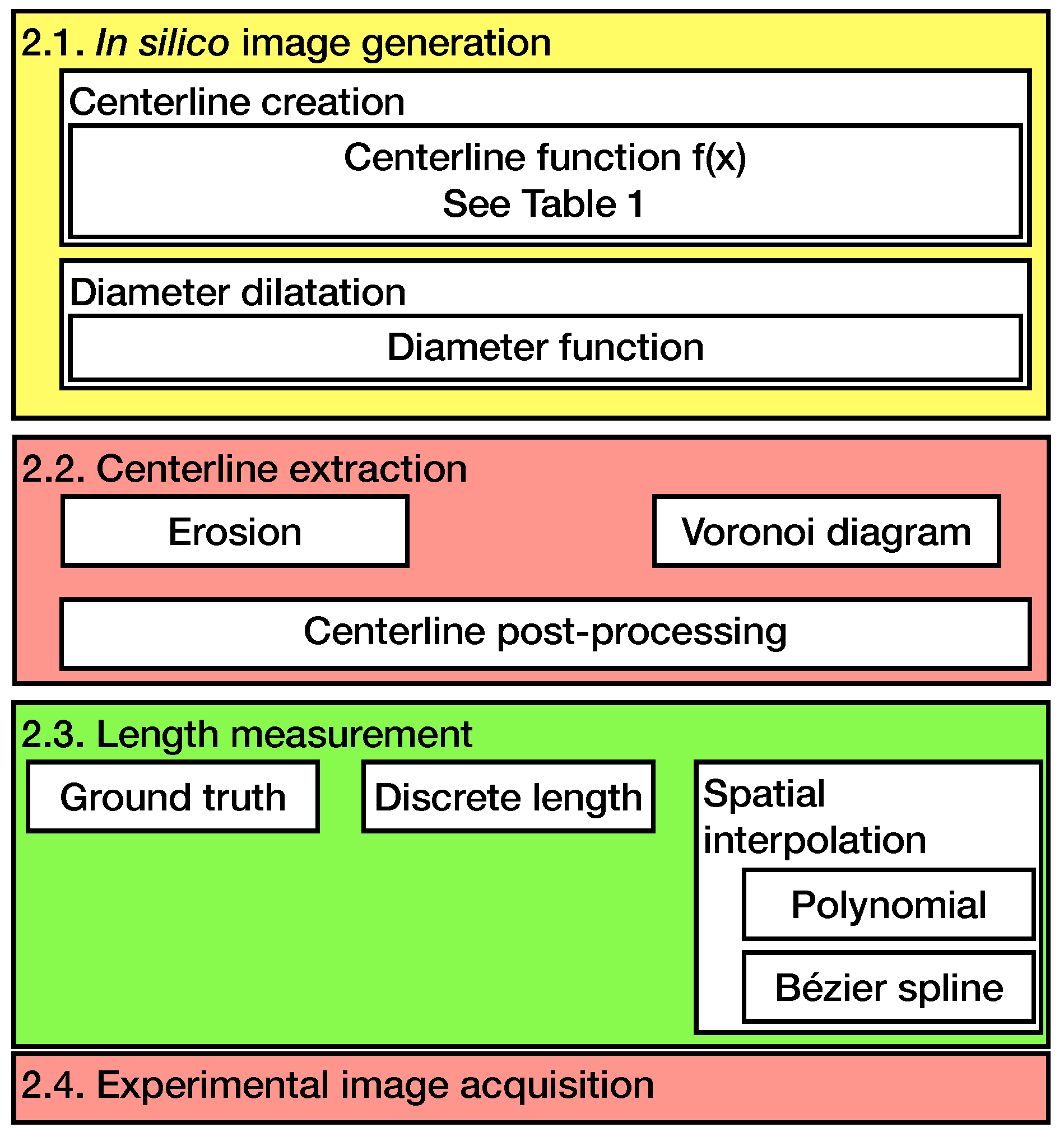
The order and structure of the methods used in this paper are sketched in Figure 1.

Since the in silico model was already introduced in a previous paper, only an overview of the model is given and the modifications of the published model are presented in the following section [25]. The centerline extraction and spatial interpolation methods are described. It is followed by the validation in a physical experiment and the evaluation method.

2.1. In-Silico Model

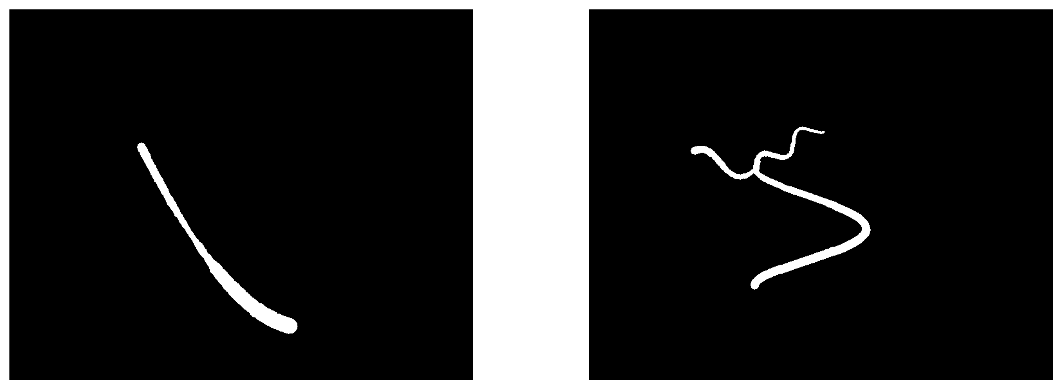
The model generates binary images mimicking a broad range of possible vessel segmentations. The generation is based on mathematical functions where the geodesic length is extracted as arc length therefore providing a reliable ground truth. No publication is known to the authors describing vessels by mathematical functions. The proposed functions in

Table 1. Mathematical function, their formula and variables [25].

Function Type	Detailed Type	Formula	Variables’ Limit
Straight lines		$f\left(x\right)=tan\left(\theta \right)·x$	$\theta =[-{45}^{\circ },{45}^{\circ }]$, $xisarbitrary$
Parabolas	Left arm	$f\left(x\right)=a·x^2$	$a=[1,2]$
			$x_{low}=[-\sqrt{2s},-2]$, $x_{high}=[x_{low}+2,0]$
	Right arm		$a=[1,2]$
			$x_{low}=[0,\sqrt{2s}-2]$, $x_{high}=[x_{low}+2,\sqrt{2s}]$
	Vertex		$a=[1,2]$
			$x_{low}=[-\sqrt{2s},-1]$, $x_{high}=[1,\sqrt{2s}]$
	L.a. inverted		$a=[-1,-2]$
			$x_{low}=[-\sqrt{2s},-3]$, $x_{high}=[x_{low}+2,1]$
	R.a. inverted		$a=[-1,-2]$
			$x_{low}=[1,\sqrt{2s}-2]$, $x_{high}=[x_{low}+2,\sqrt{2s}]$
	V. inverted		$a=[-1,-2]$
			$x_{low}=[-\sqrt{2s},-2]$, $x_{high}=[2,\sqrt{2s}]$
Polynomials		$f\left(x\right)={\sum }_{k=4}^n{a}_k·x^k$	$n\le 15$, $x=[-5,5]$
Sinusoids	Low frequency	$f\left(x\right)=a·sin(f·\pi ·x)$	$a=[0.2s,0.7s]$, $f=[1,2]$
			$x_{low}=[0,2\pi ]$, $x_{high}=[x_{low}+0.5\pi ,x_{low}+2\pi ]$
	High frequency		$a=[0.1s,0.1+\frac{s}{2f}]$, $f=[1.5,7]$
			$x_{low}=[0,2\pi ]$, $x_{high}=[x_{low}+0.5\pi ,x_{low}+2\pi ]$
Curved Waves	Quadratic	$f\left(x\right)=q·x^2+$	$q=[-10,15]$, $a=[0.05s,0.15s]$, $f=[0.5,2]$
		$a·sin(2·\pi ·f·x)$	$x_{low}=[-3,3]$, $x_{high}=[x_{low}+2,x_{low}+6]$
	Cubic	$f\left(x\right)=c·x^3+q·x^2+$	$c=[-15,10]$, $q=[-15,30]$
		$a·sin(2·\pi ·f·x)$	$a=[0.1s,0.3s]$, $f=[0.5,2]$
			$x_{low}=[-3,3]$, $x_{high}=[x_{low}+2,x_{low}+6]$
Bell curves	Gaussian	$f\left(x\right)=a·e^{-\frac{x^2}{2{\sigma }^2}}$	$a=[0.2s,s]$, $\sigma =[0.2,3]$
			$x_{low}=[-5,1]$, $x_{high}=[1,-5]$
	G. inverted		$a=[-0.2s,-s]$, $\sigma =[0.2,3]$
			$x_{low}=[-5,1]$, $x_{high}=[1,-5]$
	Polynomials	$f\left(x\right)=a·16·$	$a=[0.2s,s]$
		$(x^4-2·x^3+x^2)$	$x_{low}=0$, $x_{high}=1$
	P. inverted		$a=[-0.2s,-s]$
			$x_{low}=0$, $x_{high}=1$
Bifurcations		Combination of all

depict a large variety of shapes and spatial frequencies. The chosen functions will be investigated separately and the results can be separated as well for the following application tailored error analysis. The functions are projected onto a resolution grid to simulate a discretization on a camera chip and then dilated to simulate segmentations. The resolution is set to 720 × 576 pixels in accordance with the PAL(DV) standard which is common in the fluorescence recording settings in most surgical microscopes. Newly released microscopes have a higher resolution but since we are proposing a software-based method, we focused on the majority of microscopes in the field. The model can be easily adjusted to an arbitrary resolution. Please note that no segmentation and projection error is included in this model. Table 1 shows the different functions. A single vessel segmentation is generated by multiple steps:

• Choose a function (randomly).
• Choose a window width s (in pixels) in the image within the limits of [65 350] (randomly) (the mathematical function will be projected into this window).
• The function will be rotated with a random angle $\alpha$.
• The windowed and rotated mathematical function will be projected onto the resolution grid and thereby discretized.

2.2. Centerline Extraction

Two centerline extraction methods were used in this work. Both methods differ in their fundamentals, are commonly used for the extraction of a centerline and will be presented in the following sections. Afterward, the necessary post-processing steps are presented.

2.2.1. Erosion

The centerline extraction by erosion is well established and used in various medical and non-medical application [26,27]. Erosion is a fundamental and iterative nonlinear operation in morphological image processing and belongs to the family of median filters. A termination condition needs to be set, in our case to preserve a closed line. Its iterative use results in a thinning of a foreground structure (logical 1) to a one-pixel thick line or even a dot in case of a circular structure. The set of elements in this paper was defined as all elements in a 3 × 3 cross neighborhood of the pixel under investigation being in the center. The termination condition was set to an asymmetrical vertical and horizontal check of the neighbors to ensure a one pixel thick centerline.

2.2.2. Voronoi Diagram

The Voronoi diagram in contrast to the erosion is not an iterative or morphological method. It is a method derived from set theory which partitions an n-dimensional space into Voronoi cells. Each Voronoi cell is defined by a center point. The cell includes all points with minimal (Euclidean) distance to this center point. If a point has an equal distance to two center points, then this point belongs to a Voronoi edge, which separates two Voronoi cells. Each point of the set belongs exclusively to one cell or edge. A Voronoi diagram is the representation of all Voronoi edges. 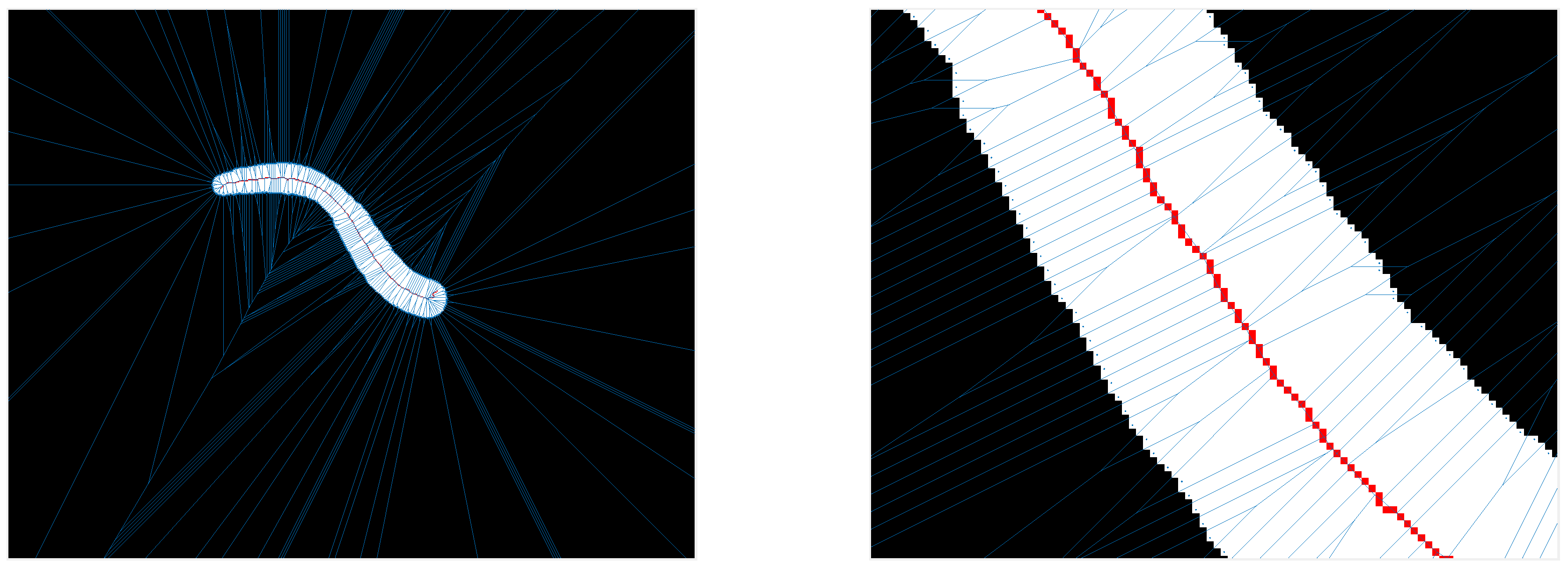They can be used to extract a centerline in 2D and 3D data sets and it was shown that it complies strongly with the Medial Axis Transformation [28]. In Figure 2 an example of a centerline extraction by a Voronoi diagram is shown. The centerline is shown in red and the Voronoi edges in blue. The set of Voronoi center points is defined as all border pixels of the segmentation mask. Two types of Voronoi edges appear, first the edges separating two neighboring Voronoi cell center points (along the segmentation border line) and second the edges separating two opposing Voronoi cell center points. These edges resulting from opposing center points represent the centerline of our given mask.

2.2.3. Centerline Post-Processing

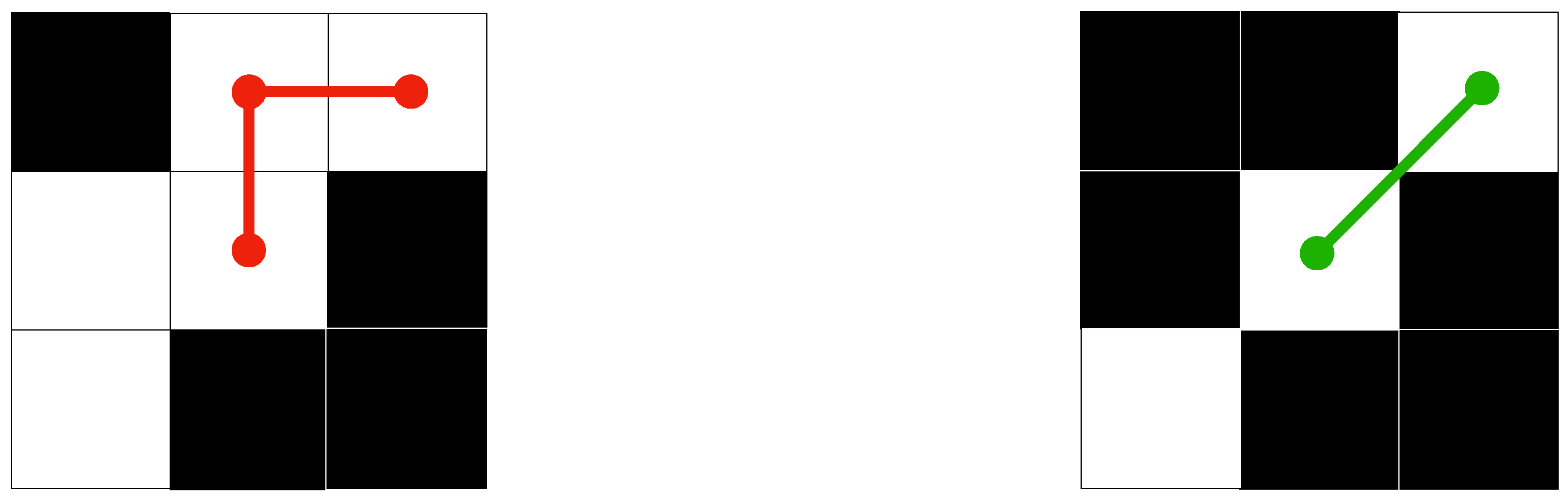
Post processing of the centerline is required before handing over the extracted centerline to the length measurement. Artifacts such as centerlines with a break of one pixel or single foreground pixels are fixed by detecting and filling or eliminating those. Afterward, a crucial step needs to be done, connections as stairway like steps are adjusted into exclusively diagonal connections. This is necessary due to the overestimation of the measured centerline in case of the appearance of orthogonal step connections as shown in Figure 3. Finally, spurs are removed at the end of the centerline.

2.3. Length Measurement

This section describes the derivation of the ground truth length from the mathematical functions, and the three length measurement methods used to calculate the length of the extracted and processed centerlines.

2.3.1. Ground Truth Length

The ground truth of the length is extracted from the mathematical function $f\left(x\right)$ as the arc length $l_{Arc}\left(f\left(x\right)\right)$ of the function $f\left(x\right)$ from $x_{start}$ to $x_{end}$ (Equation (3)). $f{}^{\prime }\left(x\right)$ is the differentiated function.

$$l_{Arc}\left(f\left(x\right)\right)={\int }_{x_{start}}^{x_{end}}\sqrt{1+f{}^{\prime }{\left(x\right)}^2}dx$$

(3)

In our case some curves are described as parametric curve by $c\left(t\right)=\left(\begin{array}{c}x\left(t\right)\\ y\left(t\right)\end{array}\right)$ which has the advantage that also bifurcations and other complex functions can be easily analyzed. The arclength is calculated as shown in Equation (4).

$$l_{Arc}\left(c\left(t\right)\right)={\int }_{t_{start}}^{t_{end}}\sqrt{x{}^{\prime }{\left(t\right)}^2+y{}^{\prime }{\left(t\right)}^2}dt$$

(4)

2.3.2. Discrete Length of Centerline

The discrete length of the obtained centerline is calculated as the sum of Euclidean distances of each pixel to its neighbor as seen in Equation (5), $l_{discrete}$ is the discrete length of the centerline, i is the index of the sorted pixels along the centerline, $i_{max}$ is the number of pixels of the centerline and $cl$ represents the centerline.

$$l_{discrete}=\sum _{i=0}^{i_{max}-1}{∥cl(i+1)-cl\left(i\right)∥}_2$$

(5)

2.3.3. Continuous Length by Polynomial Approximation

One approach to approximate a set of points by a mathematical function is the approximation with a polynomial function. In this case $x\left(i\right)$ and $y\left(i\right)$ are treated independently. A polynomial of the order 10 and all elements (number of elements = $i_{max}$) of $x\left(i\right)$ and $y\left(i\right)$ are used. The order 10 was chosen due to its versatility and adaptability since it can depict a broad range of geometries and showed good results in an explorative study prior to this work. The functions’ coefficients are determined by the least squares method by QR decomposition of the Vandermonde Matrix [29]. Afterward, both polynomials can be used to calculate the arclength of the approximated centerline (see Equation (6)).

$$l_{poly}={\int }_0^{i_{max}}\sqrt{x_{poly}{}^{\prime }{\left(t\right)}^2+y_{poly}{}^{\prime }{\left(t\right)}^2}dt$$

(6)

2.3.4. Continuous Length by Bézier Curve

Bézier curves are parametric curves with Bernstein polynomials ($B_i^n$) as the basis. The ith Bernstein polynomial of the order n is defined as:

$$B_i^n\left(x\right)=\left(\genfrac{}{}{0pt}{}{n}{i}\right)·x^i·{(1-x)}^{n-i}$$

(7)

with $x\in [0,1]$ and

$$\left(\genfrac{}{}{0pt}{}{n}{i}\right)=\frac{n!}{i!·(n-i)!}$$

(8)

A Bézier curve is a linear combination of Bernstein polynomials of the order n, weighted by the control points P as input. n equals the number of control points P. This results in the following function with $x\in [0,1]$:

$$Bezier\left(x\right)=\sum _{i=0}^n\left(\genfrac{}{}{0pt}{}{n}{i}\right)·x^i·{(1-x)}^{n-i}·P_i$$

(9)

The Bézier curve is used to approximate the reconstructed discrete centerline by a continuous function. Therefore, all elements of the centerline are used as control points for a set of k Bézier curve elements. Each curve was calculated from at least four control points, where two consecutive curves share exactly one point. A collinearity condition at the transition of two segments enforces a $C^1$ Bézier spline. This avoids too strong spatial smoothing compared to the input of all control points at once and still matches the requirement of a constantly differentiable function due to the tangential property of Bézier curves in general. The length of each curve is determined by the parametric Bézier curve elements and summed up to calculate the length of the centerline (Equation (10)).

$$l_{Bezier}=\sum _{B=1}^k{\int }_0^1\sqrt{x_B{}^{\prime }{\left(t\right)}^2+y_B{}^{\prime }{\left(t\right)}^2}dt$$

(10)

2.4. Physical Length Measurement

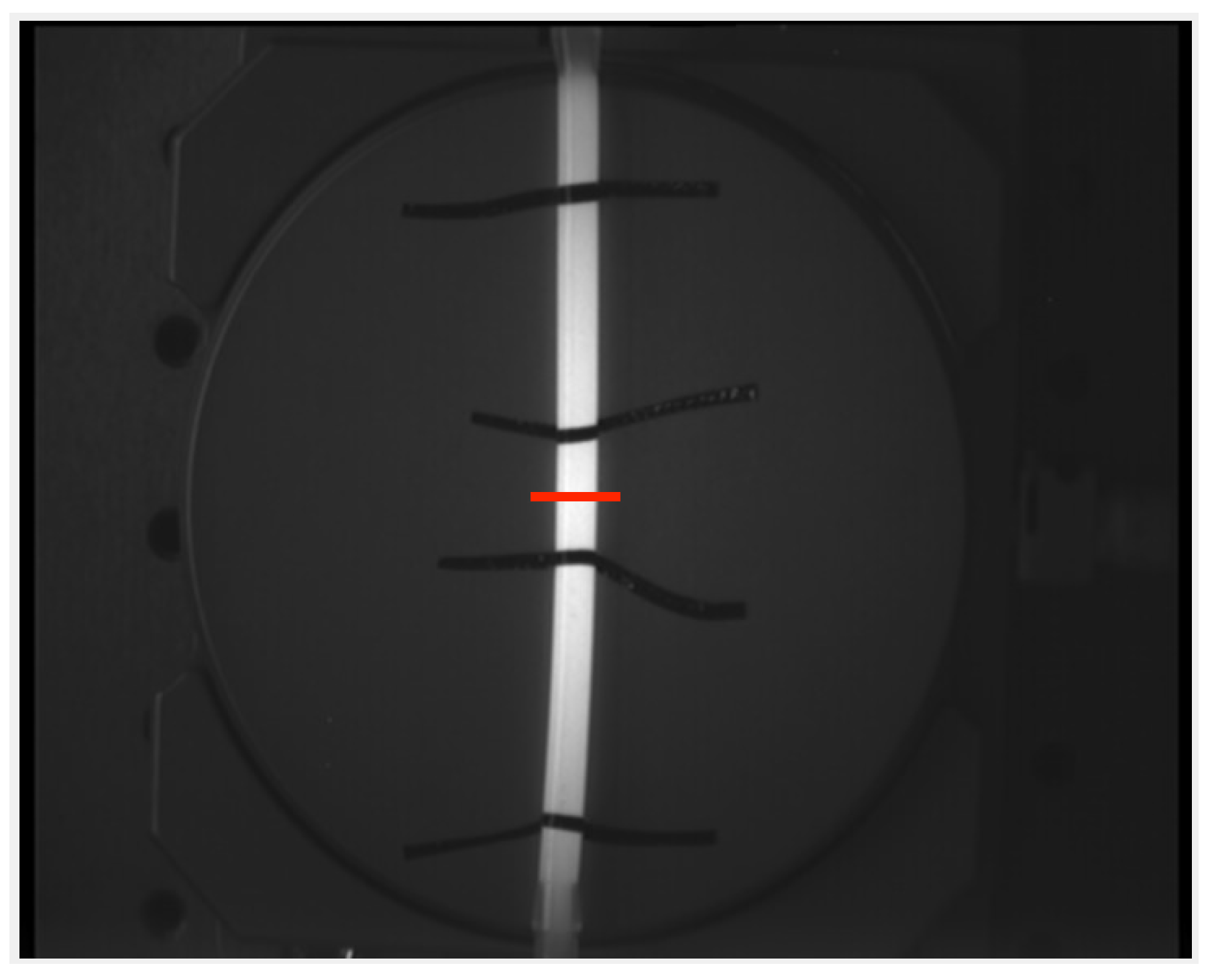
To support the findings from the in silico simulation, an experiment is set up. The possibilities in silico are very broad and easily scalable. As a proof of concept, the results of the linear functions and straight silicone tubes are compared regarding the error in geodesic length measurement. The silicone tubes have a thin wall and are filled with a solution containing the dye Indocyanine Green to ensure a high contrast while imaging with a camera and illumination setup. They are placed on a rotational plate as seen in Figure 4 and images are taken at different angles (0° to 90° in 15° steps always starting at 0°). The rotational positioning accuracy of the plate is $\pm 0.5$°. The relative position of the plate and the recording system were not changed throughout all experiments. The size of the tubes are varied as shown in

Table 2. Tubes used in the experiment.

Inner Diameter in mm	Wall Thickness in mm
1	1
2	0.5
3	0.5
4	0.5
5	0.5
6	1
7	1
8	1

. Markers are placed on the tubes to indicate the distances at which the ground truth is known. In total 56 images are recorded and then processed the same way as the in silico images.

The setup includes the following items:

• Carl Zeiss Meditec AG PENTERO^® 900 (Surgical microscope)
• Silicone tubes RCT THOMAFLUID^®
• Rotational plate (Thorlabs PR01(/M))
• Blood analog (52.4 mL demineralized water, 41.5 mL Glycerin (99.5%) and 6.7 g protein powder)
• ICG (PULSION Medical Systems SE)

2.5. Evaluation

The relative error in length measurement will be used for the evaluation of the methods. The relative error for the in silico data is calculated in reference to the continuous ground truth length (see Equation (11)).

$${ϵ}_s=\frac{l_{measured}}{l_{Arc}}-1$$

(11)

Hereby, eight values need to be tracked for each image:

• Continuous ground truth length
• Discrete ground truth length without any centerline reconstruction
• Discrete length with the centerline reconstruction by erosion
• Discrete length with the centerline reconstruction by Voronoi diagram
• Continuous length with the centerline reconstruction by erosion and interpolation by Bézier
• Continuous length with the centerline reconstruction by erosion and interpolation by polynomial approximation
• Continuous length with the centerline reconstruction by Voronoi diagram and interpolation by Bézier
• Continuous length with the centerline reconstruction by Voronoi diagram and interpolation by polynomial approximation

The ground truth in the physical experiments is the hand measured distance between the markers using a micrometer caliper with an indication accuracy of 10 $\mathsf{\mu }$m (Stahlwille 77371002). From three measurements the mean was calculated and used for the error calculation. The deviation in the measurement of the ground truth with the caliper was in the magnitude of 0.1% or less of the length of the segments in all cases. The caliper was zeroed and reapplied between each single measurement.

Since showing all results is not feasible the mean $\mathsf{\mu }$ and standard deviation $\sigma$ of the relative errors will be given for all structures separately and accumulated. A positive error indicates a measurement longer than the ground truth and a negative error shorter. Finally, a two sided Wilcoxon rank sum test is performed to proof significant changes after re-continualization of the discrete centerline. The significance level will be denoted by an asterisk in the corresponding tables.

3. Results

The results are split in two parts, first the results from in silico analysis and second the experimental results.

3.1. In Silico Results

Figure 5 shows two examples of vessel segmentations generated by the in silico model. The centerline extraction and spatial interpolation methods were then applied on 1204 such images.

Table 3. Mean relative error of the discrete length measurement with no reconstruction compared to the continuous ground truth [25].

Function Type	Relative Error	Quantity in the Set
Straight lines	2.3%	184
Parabolas	7.2%	312
Polynomials	6.3%	168
Sinusoids	6.8%	132
Curved Waves	7.6%	102
Bell curves	8.5%	108
Bifurcations	6.7%	198
Mean of all	6.3%

shows the discretization error of the mathematical functions, which is due to the projection onto the grid. No reconstruction methods were used here, and all errors are positive. Furthermore, the quantity of images in each set is shown.

Table 4. Mean relative error of the length measurement methods in % after centerline extraction by erosion compared to the continuous ground truth. Significance was proven for the reduction of the error compared to the discrete length for each function type ${}^{****}$ p < 0.0001.

	Discrete μ ± σ	Bézier μ ± σ	Polynomial μ ± σ
Straight lines	5.2 ± 3.8	2.6 ± 1.8 ${}^{****}$	2.1 ± 1.6 ${}^{****}$
Parabolas	7.5 ± 4.0	2.4 ± 1.5 ${}^{****}$	1.9 ± 1.3 ${}^{****}$
Polynomials	6.5 ± 4.8	3.9 ± 6.2 ${}^{****}$	7.2 ± 7.5 ${}^{****}$
Sinusoids	8.5 ± 5.8	4.2 ± 7.8 ${}^{****}$	6.6 ± 12.6 ${}^{****}$
Curved waves	7.6 ± 2.6	2.5 ± 1.4 ${}^{****}$	2.6 ± 2.2 ${}^{****}$
Bell curves	10.4 ± 3.2	3.1 ± 1.7 ${}^{****}$	1.9 ± 1.4 ${}^{****}$
Bifurcations	6.1 ± 5.4	2.1 ± 5.3 ${}^{****}$	2.6 ± 5.1 ${}^{****}$
Mean of all	7.0 ± 4.8	2.7 ± 4.5 ${}^{****}$	3.2 ± 5.8 ${}^{****}$

shows the comparison of the spatial interpolation methods for the centerline extraction by erosion for all used mathematical functions. It should be noted that the mean error due to discretization after the centerline extraction is 7.0% and the best interpolation method (Bézier) reduces this error to 2.7%.

Table 5. Mean relative error of the length measurement methods in % after centerline extraction by Voronoi diagrams compared to the continuous ground truth. Significance was proven for the reduction of the error compared to the discrete length for each function type ${}^{****}$ p < 0.0001.

	Discrete μ ± σ	Bézier μ ± σ	Polynomial μ ± σ
Straight lines	5.1 ± 5.8	3.3 ± 5.8 ${}^{****}$	3.2 ± 6.0 ${}^{****}$
Parabolas	8.6 ± 7.0	4.2 ± 8.5 ${}^{****}$	4.5 ± 8.7 ${}^{****}$
Polynomials	9.1 ± 8.5	7.7 ± 11.0 ${}^{****}$	11.2 ± 11.3 ${}^{****}$
Sinusoids	8.6 ± 5.0	5.6 ± 7.8 ${}^{****}$	8.9 ± 12.8 ${}^{****}$
Curved waves	8.3 ± 4.5	4.5 ± 7.0 ${}^{****}$	5.7 ± 7.5 ${}^{****}$
Bell curves	8.2 ± 4.2	3.4 ± 5.1 ${}^{****}$	3.4 ± 5.6 ${}^{****}$
Bifurcations	7.9 ± 11.2	4.6 ± 11.6 ${}^{****}$	5.9 ± 11.2 ${}^{****}$
Mean of all	7.9 ± 8.1	4.7 ± 9.2 ${}^{****}$	5.9 ± 10.0 ${}^{****}$

shows the comparison of the spatial interpolation methods for the centerline extraction by Voronoi diagrams for all used mathematical functions. The mean error due to discretization after the centerline extraction is 7.9% and the best interpolation method (Bézier) reduces this error to 4.7%.

The mean run time for the combination of the two reconstruction and interpolation methods is shown in

Table 6. Mean run time of the different combination of the methods in seconds for a single image.

	Erosion	Voronoi
Bézier curve	13.08 s	21.09 s
Polynomial approximation	2.33 s	10.34 s

. The erosion method with polynomial approximation was the quickest and the Voronoi diagram in combination with the Bézier curve the slowest. The difference was approximately a factor of ten. The measurement of the discrete length was neglected due to an unacceptable performance in length measurement. The run time was determined on a computer with an Intel i5-Quad-Core Processor with 3.4 GHz with no parallel computing.

3.2. Experimental Results

The deviation in the measurement of the ground truth with the caliper was in the magnitude of 0.1% or less of the length of the segments in all cases. The experiments on the silicone tubes resulted in the mean length errors, which are shown in

Table 7. Mean relative error of the length measurement methods in % after the centerline extraction by both methods and the spatial interpolation compared to the ground truth for the experimental data set (mean also over all angles). Significance was proven for the reduction of the error compared to the discrete length for each function type ${}^{****}$ p < 0.0001. Angle resolved relative errors are given in Table 8 and Table 9.

	Discrete μ ± σ	Bézier μ ± σ	Polynomial μ ± σ
Erosion	4.7 ± 3.0	1.9 ± 1.3 ${}^{****}$	1.6 ± 1.6 ${}^{****}$
Voronoi	5.0 ± 3.0	2.0 ± 1.3 ${}^{****}$	1.5 ± 1.5 ${}^{****}$

. Please note that these errors represent the mean error for all angles.

The tubes were set up as lines in different angles.

Table 8. Mean relative error of the length measurement methods in % after the centerline extraction by erosion and the spatial interpolation compared to the ground truth for the experimental data set. Significance was proven for the reduction of the error compared to the discrete length as indicated ${}^{*}$ p < 0.05, ${}^{***}$p < 0.001, ${}^{****}$ p < 0.0001.

	Discrete	Bézier	Polynomial
Angle	μ ± σ	μ ± σ	μ ± σ
0°	2.4 ± 1.3	1.8 ±1.5 ${}^{*}$	1.5 ± 1.5 ${}^{***}$
15°	7.0 ± 2.4	2.3 ± 1.0 ${}^{****}$	1.7 ± 1.6 ${}^{****}$
30°	6.6 ± 2.3	1.9 ± 1.3 ${}^{****}$	1.6 ± 1.6 ${}^{****}$
45°	2.2 ± 1.7	1.6 ± 1.6 ${}^{*}$	1.6 ± 1.7 ${}^{*}$
60°	7.0 ± 2.3	1.8 ± 1.3 ${}^{****}$	1.4 ± 1.6 ${}^{****}$
75°	5.8 ± 2.6	2.1 ± 1.2 ${}^{****}$	1.9 ± 1.7 ${}^{****}$
90°	1.9 ± 1.3	1.7 ± 1.6	1.6 ± 1.7

and

Table 9. Mean relative error of the length measurement methods in % after the centerline extraction by Voronoi diagrams and the spatial interpolation compared to the ground truth for the experimental data set. Significance was proven for the reduction of the error compared to the discrete length as indicated ${}^{*}$p < 0.05, ${}^{**}$p < 0.01, ${}^{***}$p < 0.001, ${}^{****}$ p < 0.0001.

	Discrete	Bézier	Polynomial
Angle	μ ± σ	μ ± σ	μ ± σ
0°	2.4 ± 1.6	1.8 ±1.3	1.5 ± 1.4 ${}^{*}$
15°	7.4 ± 2.3	2.6 ± 1.0 ${}^{****}$	1.6 ± 1.2 ${}^{****}$
30°	6.8 ± 2.2	2.1 ± 1.3 ${}^{****}$	1.7 ± 1.6 ${}^{****}$
45°	2.5 ± 1.5	1.6 ± 1.5 ${}^{**}$	1.5 ± 1.6 ${}^{***}$
60°	7.1 ± 2.2	1.9 ± 1.1 ${}^{****}$	1.5 ± 1.5 ${}^{****}$
75°	6.4 ± 2.2	2.3 ± 1.0 ${}^{****}$	1.5 ± 1.6 ${}^{****}$
90°	2.3 ± 1.7	1.7 ± 1.5	1.5 ± 1.6 ${}^{**}$

and Figure 6 show the relative error in dependency to the angle (relative to the resolution grid). The discrete centerline shows, as expected, a clear dependency on the angle with the minimum error at 0°, 45° and 90° where the centerline best fits into the camera chip grid.

4. Discussion and Conclusions

The proposed model is able to generate a large number of images mimicking pre-segmented cerebral vessels with a mathematically defined ground truth. The multitude of shapes including bifurcations depict a large variety of possible vessel structures. No publication is known to the authors describing vessel geometries by mathematical functions. Therefore, some of the proposed functions and their parameters’ limits might be suitable and others unsuitable to describe a vessels geometry. The functions used in this model can be considered separately and therefore also the findings derived from the results as well. Validation of the model and the used functions requires an in vivo data set, including processing of the data, which is also a source of bias and error. Nevertheless, the model is designed to depict an extensive range of vessel geometries and a retrospective containment is possible. The focus of this paper was the measurement of the geodesic length along the centerline. It adds value to the previous publication by the authors [25] by extending the investigation of the discretization error of a continuous object by the development of counteractions and the investigation of their effectiveness to reduce this error in silico and in a physical experiment. We have first shown that the error due to discretization of the ground truth centerline is +6.3%. No reconstruction method was involved in this step and the simulation is set up with the PAL(DV) standard. This error is also always positive. The error of the discrete centerline reconstructed by the proposed methods increased to 7.0% and 7.9% (Erosion and Voronoi method). This is intuitive, since the error due to the reconstruction adds up to the discretization error. According to Equation (2), the propagated error from length measurement is directly forwarded as an element of the sum. Assuming the same error for the diameter measurement, the relative error in the flow measurement would result in 21.0% and 23.7% for the erosion and Voronoi method. In fact, the error is even higher because the model does not account for segmentation errors or projection errors of a 3D structure onto a 2D plane. This projection error is strongly dependent on the angle between the vessel segment and focal plane. It can be described by a cosine function $cos\left(\alpha \right)=\frac{l_{projection}}{l}$. Small changes in $\alpha$ result in small projection errors and are tolerable. A tilt angle of approximately ±16° would equalize the positive effect of the re-continualization by the proposed methods. In a clinical context a tilt angle of 16° is not expected. The depth of field in typical neurovascular surgery is smaller than 2 mm (at a magnification of >7) [30]. Consequentially, any vessel larger than 7 mm would be partially blurry. Nevertheless, requirements on the measurement work flow can be derived to ensure that the projection error does not equalize the gained accuracy in length measurement. These propagated error values do not include errors from transit time measurement and are already too high. For comparison, sonographic contact intraoperative flow meters have an accuracy of ±10% [12]. This emphasizes the need for an improved geodesic length assessment method to enable a reliable optical volume flow measurement. One option is changing the hardware and using a camera with a higher spatial resolution. Unlike the coastline paradox, where the length of a fractal object is prolonged towards infinity with increasing resolution, we expect a convergence of the measured geodesic length towards the true length with increasing resolution. This is due to the decreasing discretization error. It relies on the assumption that a vessel is a non-fractal object. This assumption is most likely valid for vessels (probably not for the capillary system). The upgrade of the recording system is costly and cannot be easily performed on systems already in use and therefore it is not the prioritized solution. Another option is using software-based methods to enhance the length measurement. Re-continualization methods such as spatial interpolation to ensure in the prevalent cases a smooth centerline is the preferred choice since they can be easily installed to all systems. The length measurement of discrete objects has shown to be longer than the continuous ground truth due to the angular characteristic of the pixels as a grid. Some outlier cases are shorter. Either the reconstruction or the spatial interpolation of the centerline introduces a negative error. We have observed that the reconstruction of the centerline can provoke negative errors due to a wrong spur removal at the ends of the centerline, especially in the case of bifurcation. Whether the spatial interpolation introduces a negative error is checked by applying it to the discrete ground truth centerline (no reconstruction involved) and comparing the resulting length with the continuous length of the centerline. This showed a mean relative error of <0.05% for the Bézier curves method, which emphasizes its suitability to properly re-continualization a discrete centerline without too strong spatial smoothing. The polynomial approximation showed a mean relative error of approximately $-2\%$. This implies a strong spatial smoothing caused by the limited capability of polynomial functions to represent different and versatile structures. Here the order of the polynomial has a large influence since a small order could provoke a strong smoothing and a large order could introduce spikes and therefore lengthen the centerline. Taking into account that a centerline consists of hundreds of elements, a not piecewise fitted function (as the polynomial fit is) is prone to extensive smoothing effects. Therefore, the proposed method using Bézier curves is more robust.

All proposed centerline extraction methods and their combination with spatial interpolation methods show a significant decrease in the relative error in length measurement. This verifies the first hypothesis and validates the proposed approach. Especially the centerline extraction by erosion in combination with the Bézier curve interpolation shows a significant decrease in error from 7.0% to 2.7% (compared with the discrete centerline obtained by reconstruction). The run time of approximately 13 s per image on average is acceptable since the operation is not required to be in real time. Furthermore, the code runs on MATLAB and not on an optimized processor and solver, so a further decrease in run time is possible. The run time was tracked to evaluate the methods relative to each other and not in an absolute manner. The evaluation of the recorded images of silicone tubes comply with the in silico simulation and show similar errors with their respective counterpart (straight lines). The physical experiments are prone to several sources of errors. First, the positioning accuracy of the sample in the field of view contains errors. The translational displacement was avoided by fixing the imaging system and the rotational plate. The rotational positioning was set by a rotational plate with an accuracy of $\pm 0.5$°. 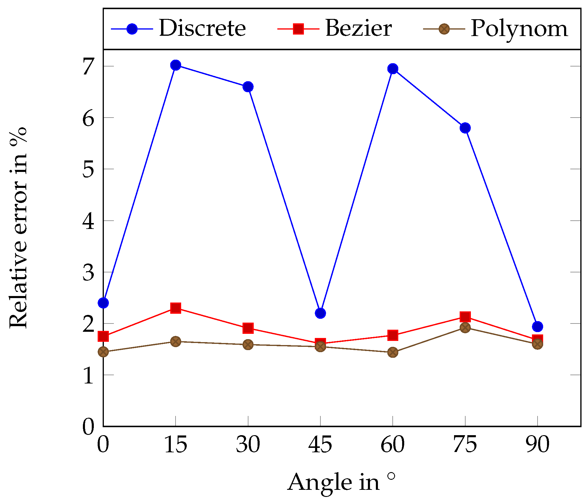A value of this magnitude induces a minor error in length measurement even at the most sensitive angle changes (see Figure 6). Second, the manual measurement of the ground truth length with a caliper introduces errors. The caliper has an indication accuracy of 10 $\mathsf{\mu }$m, which introduces a small error. The measured segments yield lengths from 12–75 mm and are much larger than this error. Furthermore, the repeated measurement with the caliper showed a good reproducibility with a deviation of 0.1% or less. In conclusion, all errors are small and do not have a large impact on the measurement and therefore the results of the physical measurement are assumed trustworthy. The results of this investigation also verifies the second hypothesis. The rectangular grid of the detection array leads to an angle dependent error, which is reduced by re-continualization. The angular measurements (Table 8 and Table 9 and Figure 6) show a clear dependency of the error in length in case of a discrete measurement. The measurements also show that the re-continualization by spatial interpolation significantly reduces this error in nearly all cases. The reduction is more significant in the cases of angles that do not fit the grid (15°, 30°, 60° and 75°). This implies that the dependency of the error to the angle is reduced. It is not possible to recreate all in silico categories with silicone tubes since the geometry of the tubes changes when they are bent. Three-dimensional printed structures could overcome this drawback but an investigation of the tolerances of the printers is required. The results of this research are of great importance for applications where small changes in the measurement have a significant impact on the outcome. Especially in medicine and life science, errors can have fatal consequences for the patient. Facilitating a non-contact flow measurement with an acceptable accuracy would fit into the surgical work flow. It would also increase the quality of the procedure and could decrease the recurrence rate. Further, the results are also applicable in all fields where geodesic distances of discretized images are requested with a high precision.

5. Outlook

The proposed model depicts a broad range of vessel geometries. Its validation requires a sufficient in vivo data set. Its validation on different images could help to clarify which mathematical functions are the most suitable for length analysis. This also leads into an application tailored model (e.g., retinal vessel have different geometries than cerebral vessels). So far, this model does not account for the projection errors of a 3D object onto a 2D plane. Adding a dimension to the mathematical functions is possible. This would not only enable the inclusion of projection errors into the investigation, it would also enable 3D length analysis (for example, of 3D—Computed Tomography (CT) or Magnetic Resonance Imaging (MRI) data sets).

The evaluation of the performance of the proposed length measurement techniques could be extended by a displacement analysis. In this work we focused on the length but not on the displacement. Calculating the difference of the integrals (mathematical input function and Bézier curve) could exploit circumstances that limit the error reduction by re-continualization.

The developed model can also be used to determine the performance of hardware-based methods to lower the discretization error. Changing the resolution in the model is easy and a follow up study can be performed to assess the benefits of increasing the resolution. Requirements on the resolution could be derived from this assessment and the required applicative specifications. Finally, non-geometrical factors need to be analyzed to complete the error analysis. This could be done analogously with the help of synthetic images or in measured data. Once in silico studies are done, ex vivo and in vivo studies are needed to finally state the accuracy and tolerances of the optical measurement of volume flow in clinical use.