Exploiting the Nonlinear Dynamics of Optically Injected Semiconductor Lasers for Optical Sensing

Abstract

Optically injected semiconductor lasers are known to display a rich variety of dynamic behaviours, including the emission of excitable pulses, and of rare giant pulses (often referred to as optical rogue waves). Here, we use a well-known rate equation model to explore the combined effect of excitability and extreme pulse emission, for the detection of variations in the strength of the injected field. We find parameter regions where the laser always responds to a perturbation by emitting an optical pulse whose amplitude is above a pre-defined detection threshold. We characterize the sensing capability of the laser in terms of the amplitude and the duration of the perturbation.

1. Introduction

Complex dynamical systems often exhibit extreme or rare events. Examples in nature include earthquakes, hurricanes, financial crises, and epileptic attacks, to name just a few [1]. In recent years the generation of extreme events in optical systems has attracted attention [2,3], as such systems serve as experimental platforms for testing the physics of extreme event generation in a controlled environment, where parameters can be tuned with high precision. In particular, the dynamics of continuous-wave (cw) optically injected semiconductor lasers has attracted attention, because, under appropriated conditions, the laser can emit excitable pulses [4,5], or rare giant pulses [6]. Thus, the cw optically injected laser has been used for testing methods either to suppress [7] or to generate “on demand” [8] high optical pulses. In addition, in contrast to what can be achieved in other fields, optics laser systems allow to record long datasets containing large numbers of extreme events. Such optical “big data” has also been used for testing data analysis tools for extreme event prediction [9,10,11].

Here, we study the optical pulses emitted by a cw optically injected laser with a different motivation: we aim at exploiting the capability of high-pulse emission for implementing a laser-based sensor, able to detect perturbations of the strength of the injected optical field. Let us assume, for example, an optical perturbation due to the presence, during a certain time interval, of gas molecules in the beam path from the pump laser (master) to the injected laser (slave) which, due to light absorption, decrease the injected power. We aim to find appropriated conditions such that the decrease of the injected power triggers the emission of an optical pulse, high enough to cross a pre-defined “detection threshold”. In order to precisely detect the optical perturbation, the emission of the pulse should occur shortly after the injected power decreases, i.e., within a pre-defined “detection time interval”. In this way, the high pulse emitted will allow detecting the presence of gas molecules in the master-slave beam path. In other words, our goal is to exploit the laser excitable response for the detection of a variation of a control parameter, specifically, the decrease of the injected power. In order to avoid the detection of “false positives” we consider parameters such that the laser intensity, under constant injection conditions, is either constant or displays small oscillations, below the detection threshold. We show that for appropriated parameters, the decrease of the injected power can be reliably detected as it will trigger, with probability equal or close to one, the emission of a pulse, high enough to cross the detection threshold, and emitted shortly after the perturbation begins (i.e., within the detection time interval).

This paper is organized as follows. Section 2 presents the model equations, Section 3 presents the numerical results and Section 4 presents the discussion.

2. Model

The equations describing the dynamics of an optically injected semiconductor laser are [12,13,14]:

$$\begin{array}{ccc}\hfill \frac{dE}{dt}& =& \kappa (1+i\alpha )(N-1)E+i\Delta \omega E+\sqrt{P_{inj}},\hfill \end{array}$$

(1)

$$\begin{array}{ccc}\hfill \frac{dN}{dt}& =& {\gamma }_N{(\mu -N-N|E|}^2).\hfill \end{array}$$

(2)

Here E is the slow envelope of the complex optical field, $S={\left|E\right|}^2$ is the intensity, N is the carrier density, $\kappa$ is the field decay rate, $\alpha$ is the line-width enhancement factor, and ${\gamma }_N$ is the carrier decay rate. $\Delta \nu =\Delta \omega /2\pi$ with $\Delta \omega ={\omega }_s-{\omega }_m$ is the frequency detuning between the slave laser and the master laser, $P_{inj}$ is the injection strength and $\mu$ is the injection current parameter (normalized such that the threshold of the free-running laser is at ${\mu }_{th}$ = 1).

We consider a decrease of $P_{inj}$ at time $T_p$ that has a Gaussian temporal shape centered at $T_p$, amplitude, $\Delta P$, and duration, $\Delta T$: $P_{inj}\left(t\right)=P_0-\Delta Pexp[-{(t-T_p)}^2/(2\Delta T^2)]$. To avoid numerical problems we take $P_{inj}=P_0$ constant for $t>>T_p$ and $t<<T_p$.

We note that spontaneous emission noise is not included in the model. This is because noise can trigger the emission of pulses, which will lead to false detections. Further testing using realistic noise levels is of course necessary, in order to find model parameters such that the laser-based sensor is robust to noise. This requires that the laser dynamics have reduced sensitivity to random fluctuations [15], while it has enhanced sensitivity to deterministic perturbations of the injected optical field [16].

3. Results

The model was simulated with a 4th order Runge–Kutta method with an integration step of 1 ps and the parameters indicated in

Table 1. Parameters used in the model simulations [6].

Name	Symbol	Value
Field decay rate	$\kappa$	300 ns${}^{-1}$
Line-width enhancement factor	$\alpha$	3
Carrier decay rate	${\gamma }_N$	1 ns${}^{-1}$
Injection current parameter	$\mu$	$1.96$
Frequency detuning	$\Delta \nu$	variable
Unperturbed injected Power	$P_0$	variable
Perturbation amplitude	$\Delta P$	variable
Perturbation duration	$\Delta T$	variable
Detection time interval	$\Delta T_{det}$	variable

. In order to find appropriated injection parameters, first we varied $\Delta \omega$ and $P_{inj}=P_0$ (no perturbation was applied, i.e., $\Delta P=0$), and for each set of parameters long time traces of the intensity dynamics were simulated (5 $\mu$s), and the maximum, $I_{max}$, and the average, $〈I〉$, intensity value were calculated.

The results are presented in Figure 1 which displays, in color code, the relative height of the intensity oscillations, $\Delta I=I_{max}-〈I_{max}〉)/〈I_{max}〉$ (where $I_{max}$ is the height of the highest peak found, and $〈I_{max}〉$ is the average peak height) as a function of $\Delta \nu$ and $P_{inj}$. The dark regions indicate either injection locking (in the region starting at $\Delta \nu =0$, right of the red-orange central region, the intensity is constant and there are no oscillations, $I_{max}=〈I_{max}〉=0$) or period-one solutions (in the dark region to the left of the red-orange region the intensity dynamics consists of regular oscillations, all the intensity peaks are equal, $I_{max}=〈I_{max}〉$ and $\Delta I=0$).

To operate the laser as a sensor, we need to select an appropriated detection threshold, $TH$, such that when the injected optical power is constant, the laser intensity is either constant, or displays oscillations which are always below the detection threshold. In this way, we avoid the detection of “false positives”: if $P_{inj}$ is constant, $I\left(t\right)<TH$ ∀ t. In Figure 1 we see that $\Delta I<4$. Therefore, we chose a detection threshold proportional to the mean value of the height of the peaks, $TH=(1+c)〈I_{max}〉$, with $c\le 4$ being a constant that depends on the parameters. We exclude parameters for which the distribution of intensity values is long-tailed (i.e., where the laser emits rare giant pulses [6]), because for such parameters, a very high threshold will be needed in order to avoid false detections; however, a very high threshold might not detect some of the pulses that can be emitted in response to variations of $P_{inj}$. In the following we consider the following parameters: $P_0=50$ ns${}^{-2}$, $\Delta \nu =-2.29$ GHz (indicated with a circle in Figure 1) which are close to the boundary of the region where large pulses are emitted, and arbitrarily fix the threshold to $TH=2〈I_{max}〉$ (while a systematic study is needed to determine the optimal choice, our simulations suggest that the results are robust with respect to small variations of the threshold).

Figure 2 displays two examples of the intensity time series together with the perturbation of the injected power. If, within a given detection time interval, $\Delta T_{det}$, the emitted pulses are below the threshold $TH$, the perturbation is not detected (panel a), but if at least one pulse is above $TH$, the detection is successful (panel b). As it will be discussed latter, $\Delta T_{det}$ is an important parameter of the detection system. It starts when $P_{inj}$ decreases below a given percentage of $P_0$, here taken as 20%.

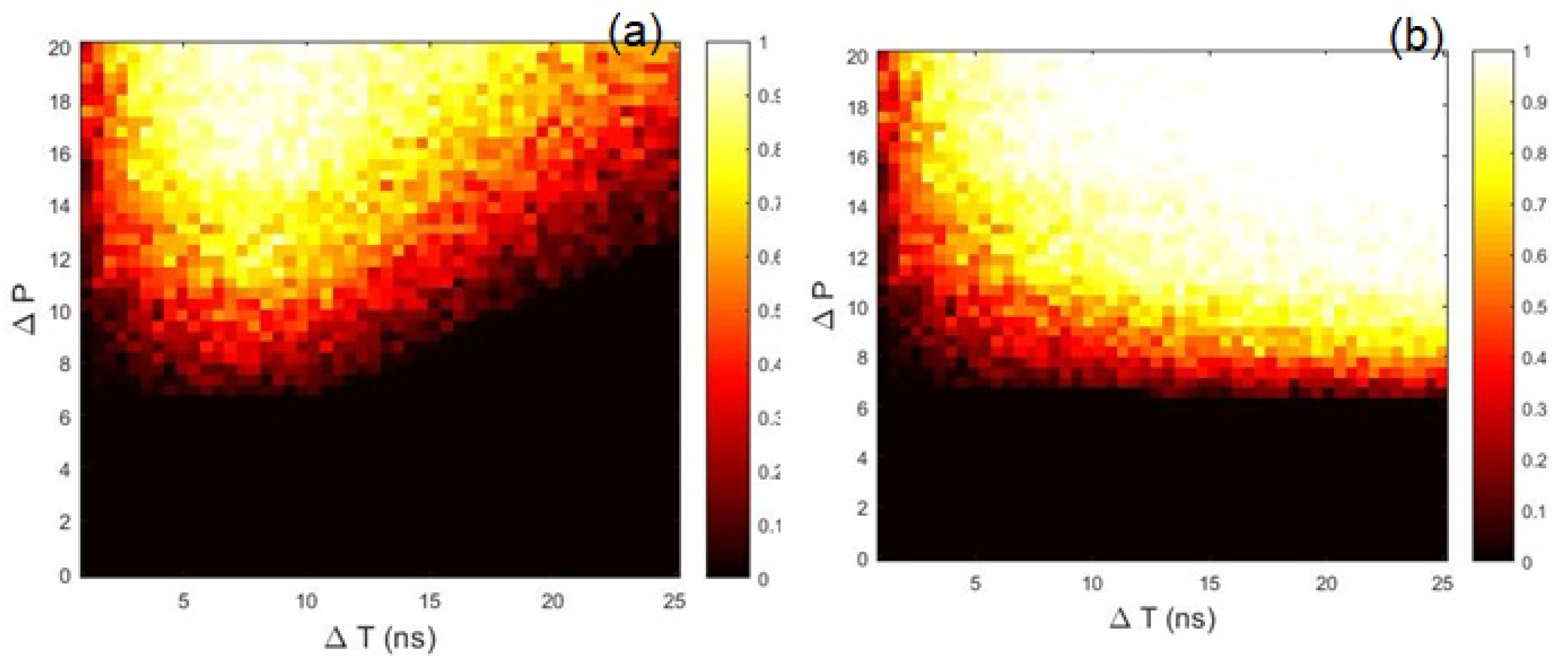
In order to characterize the sensing capability of the laser, we analyze the effect of the perturbation parameters: the amplitude, $\Delta P$, and the duration, $\Delta T$. Figure 3 displays the success rate, $SR$, which is the percentage of successful detections, as a function of $\Delta P$ and $\Delta T$. In this plot, the $SR$ is computed from 50 time-series with random initial conditions, and we have verified that a larger number of simulations give very similar results. We note that if the duration of the perturbation is too short, in general the detection fails because the laser has no time to respond to the perturbation by emitting a pulse that is high enough. In the other limit, if the duration of the perturbation is too long, the detection also fails, now due to the fact that the detection time interval, $\Delta T_{det}$ is too short and the laser emits a pulse at a later time. In between these two limits (if the duration of the perturbation, $\Delta T$, is not too slow nor too long with respect to the laser response time and to the detection time interval), we see in Figure 3 that the success rate is close to 1. By increasing $\Delta T_{det}$ we improve the detection of slow perturbations, however, the minimum perturbation amplitude that is detected remains nearly unchanged. This is a consequence of the excitable nature of the dynamics: the perturbation has to be strong enough to trigger a response.

As shown in Figure 4 and Figure 5 the boundary between $SR=0$ and $SR=1$ can be very sharp: if the perturbation $\Delta P$ is small and $P_{inj}$ remains above a certain value (here $P_{inj}>P_{inj}^{*}=43$ ns${}^{-2}$) the intensity dynamics remains unaffected. On the contrary, if the perturbation is such that $P_{inj}$ decreases below $P_{inj}^{*}$, then pulses are emitted, which can be detected by selecting appropriated values of the threshold and of the detection time interval.

4. Discussion

We have numerically studied the dynamics of an optically injected laser and have shown that, under appropriated conditions, a decrease of the injected power can be detected by the emission of optical pulses that are high enough to cross a pre-defined detection threshold, and that are emitted within a pre-defined detection time interval. The model parameters need to be chosen such that the laser intensity, under constant injected power, has a well-defined maximum value (i.e., the distribution of intensity values does not exhibit a long tail). In this case, a detection threshold can be defined such that, in the absence of perturbation, the intensity oscillations are always below the threshold, while at least one intensity pulse crosses the threshold with probability close or equal to one, if a perturbation is applied such that the injected power decreases. We have studied the limitations regarding the amplitude and the duration of the perturbation. In general, due to the excitable nature of the dynamics, the amplitude of the perturbation needs to be large enough, while its duration needs to be not too short nor too long. If the perturbation is too fast, the laser has no time to respond by emitting a pulse high enough, while if the perturbation is too long, the emitted pulse can be delayed with respect to the detection time interval.

In this study we have considered a Gaussian shape for the perturbation, and it will be important, for practical applications, to test the performance of the sensor using different shapes and to analyze how the detection threshold and the detection time depend on the shape of the perturbation. We have simulated noise-free equations to avoid detecting noise-induced pulses as “false positives”. Further testing using realistic noise levels is of course necessary, in order to find model parameters such that the laser dynamics is robust to noise, while is sensitive to deterministic perturbations of the injected field. An interesting setup to analyze is that of ultra-short optical feedback [17]. Further work will probably also aim to compare the detection method proposed here, which exploits the excitable properties of the laser dynamics, with more traditional approaches for sensing.