Article

Performance Evaluation and Error Tracing of Rotary Rayleigh Doppler Wind LiDAR

1
Science Island Branch, University of Science and Technology of China, Hefei 230026, China
2
Key Laboratory of Atmospheric Optics, Anhui Institute of Optics and Fine Mechanics, Chinese Academy of Sciences, Hefei 230031, China
3
Advanced Laser Technology Laboratory of Anhui Province, Hefei 230037, China
4
School of Electronic Engineering, Huainan Normal University, Huainan 232038, China
*
Authors to whom correspondence should be addressed.
Photonics 2024, 11(5), 398; https://doi.org/10.3390/photonics11050398
Submission received: 27 March 2024 / Revised: 19 April 2024 / Accepted: 22 April 2024 / Published: 25 April 2024

Abstract

:
In the study of atmospheric wind fields from the upper troposphere to the stratosphere (10 km to 50 km), direct detection wind LiDAR is considered a promising method that offers high-precision atmospheric wind field data. In 2020, Xie et al. of the Anhui Institute of Optics and Fine Mechanics, Chinese Academy of Sciences, developed an innovative rotating Rayleigh Doppler wind LiDAR (RRDWL). The system aims to achieve single-LiDAR detection of atmospheric wind fields by rotating the entire device cabin. In 2022, the feasibility of the system was successfully validated in laboratory conditions, and field deployment was completed. Due to the structural differences between this system and traditional direct-detection wind LiDAR, performance tests were conducted to evaluate its continuous detection capability in outdoor environments. Subsequently, based on the test results and error analysis, further analysis was carried out to identify the main factors affecting the system’s detection performance. Finally, the error analysis and traceability of the detection results were conducted, and corresponding measures were discussed to provide a theoretical foundation for optimizing the performance of RRDWL.

1. Introduction

Wind is a physical phenomenon on Earth that involves the horizontal movement of air, describing the motion of air currents. In scientific terms, wind is described as the moving component of air, encompassing both wind speed and wind direction. As a significant concept in meteorology, a wind field refers to the distribution of wind speed and wind direction at various positions in the atmosphere during a specific time and within a particular spatial range. The study of atmospheric wind fields has its roots in long-term observations and explorations of weather, climate, and atmospheric motions. Accurate understanding and prediction of weather conditions are crucial for human life, agriculture, transportation, aviation, and other aspects [1,2,3,4,5]. Currently, there is a widespread recognition of the significance of measuring the tropospheric wind field in improving the accuracy of numerical weather prediction and wind shear warnings. The stratosphere, located above the troposphere and extending from approximately 10 km to 50 km in height, plays a vital role in the climate system and atmospheric stability. Therefore, the importance of measuring the stratospheric wind field cannot be overlooked.
However, atmospheric wind fields exhibit complex non-uniformity and spatiotemporal variability. Wind speed and wind direction can vary significantly at different altitudes, geographical locations, and over time. This non-uniformity poses challenges in accurately measuring and depicting the complete wind field. Weather conditions, terrain, and environmental factors also play important roles in limiting wind field detection. For instance, strong winds, precipitation, cloud cover, and complex terrain can all result in incomplete and inaccurate observational data. Additionally, the detection of wind fields requires the use of multiple measurement devices and techniques; however, different equipment and methods have limitations in terms of measurement range, resolution, accuracy, and reliability [6,7,8,9,10]. In summary, the characterization of wind fields is a complex task due to these factors. Light Detection and Ranging (LiDAR) is an advanced technology that utilizes laser beams and scattered light for precise measurement and observation. In comparison to traditional meteorological sounding methods, LiDAR offers the advantage of non-contact observations, allowing for a wider range of measurements, including higher altitude levels and complex terrain areas [11,12,13].
Direct-detection wind LiDAR is a detection method that utilizes a frequency discriminator, also known as an optical mixer, to convert the Doppler frequency shift of aerosols or molecules caused by wind in the atmosphere into changes in light energy [14,15,16]. Based on the type of scatterers, direct-detection wind LiDAR can be categorized into three types: Mie wind LiDAR, Rayleigh wind LiDAR, and resonance fluorescence wind LiDAR. Compared to aerosol scattering, Rayleigh scattering is more prevalent and relatively stronger in the upper atmosphere. Despite the limitations in sensitivity due to the width of the molecular backscatter spectrum, Rayleigh scattering wind LiDAR can effectively detect the wind field in the global free troposphere and upper atmosphere [17,18,19]. Traditionally, direct-detection wind LiDAR has employed two methods to measure different line of sight (LOS) wind speeds. The first method involves mounting a scanning head above the LiDAR transceiver, which is rotated to achieve a cone scan. However, this approach becomes challenging for larger systems when the aperture of the receiving telescope exceeds half a meter. The required size, thickness, and weight of the scanning mirror increase rapidly, making it difficult to handle and more expensive. As a result, this method is primarily suitable for small and medium-sized systems [20,21]. In order to address the challenges of measuring high-altitude wind fields, researchers have explored an alternative approach. They have employed two large aperture LiDAR subsystems placed orthogonal to each other to measure orthogonal LOS wind speeds [22,23,24]. However, this approach introduces certain issues. Using two subsystems necessitates the use of two lasers, multiple large-aperture telescopes, and two separate detection and acquisition systems. This increases the costs of development and maintenance, as well as the complexity of calibrating and fine-tuning these precise instruments.
Based on the aforementioned background, Xie et al. from the Anhui Institute of Optics and Fine Mechanics, Chinese Academy of Sciences, have developed a rotary Rayleigh Doppler wind LiDAR (RRDWL). The system innovatively uses a rotating platform structure to detect horizontal wind fields through the overall rotation of the equipment. This design not only makes it possible for a single direct wind measurement LiDAR system to detect the atmospheric wind field but also effectively reduces the development cost of the equipment. In 2020, the system verified the feasibility of detecting atmospheric wind fields in a laboratory environment. Subsequently, the outfield construction was completed in 2022 [25,26]. However, due to the structural differences between this system and traditional direct wind LiDAR, it is necessary to evaluate its performance in the actual detection of the atmospheric wind field. In addition, due to the heterogeneity of the actual atmosphere and potential systematic errors in the system, complete consistency between detection results and simulation results cannot be achieved. Therefore, it is imperative to analyze and trace any errors in the detection results while discussing corresponding measures to establish a theoretical foundation for optimizing RRDWL’s performance.

2. RRDWL Wind Measurement Principle

2.1. Rayleigh Scattering LiDAR Equation

Since the advent of using lasers as a light source for atmospheric detection, researchers have observed the interaction between lasers and atmospheric substances, including scattering and absorption phenomena. These interactions can be categorized into different physical mechanisms such as scattering (Mie, Raman, Rayleigh), resonance fluorescence, and more. In the middle atmosphere, Rayleigh scattering is a prominent form of scattering due to the relatively low aerosol content above the boundary layer and the prevalence of small diameter molecules (less than one-tenth of the laser wavelength) in the atmosphere. Rayleigh scattering signals are stronger compared to Mie scattering signals. Furthermore, the shorter the wavelength of the laser used, the stronger the Rayleigh scattering and the greater the change in scattering cross-section. As a Rayleigh scattering LiDAR primarily used for middle atmosphere detection, the backscattered signal consists of two main components. The first is the Rayleigh scattering signal, which is generated when the laser interacts with air molecules (nitrogen and oxygen) in the atmosphere. The second is the meter scattering signal, which is generated when the laser interacts with aerosol particles suspended in the lower atmosphere. Although both types of scattering are considered elastic scattering and do not involve frequency drift, there are distinct differences in their scattering processes. During the actual detection and data inversion process, it is necessary to separate the pure Rayleigh scattering signal from the atmospheric echo signal by subtracting the aerosol Mie scattering signal using atmospheric models or empirical formulas. This is because the presence of aerosol scattering interferes with the received signal, and we aim to isolate the Rayleigh scattering signals associated with atmospheric molecules in order to accurately estimate atmospheric parameters.
The RRDWL primarily focuses on the detection of the wind field in the middle atmosphere, which includes the high troposphere and stratosphere. Therefore, it falls under the category of “Rayleigh scattering Doppler wind measurement”. Specifically, for the wind field in the middle atmosphere, direct wind LiDAR is the only method available for continuous observation. Therefore, the Rayleigh scattering LiDAR equation can be described using the following expression:
N R ( λ , z ) = P L ( λ ) Δ t h c / λ σ R ( π , λ ) n R ( z ) Δ z A z 2 T a , m 2 ( λ , z ) η ( λ ) G ( z ) + N B .
where P L represents the transmission power of the LiDAR system, Δ t represents the integration time, σ R represents the differential backscattering cross-section, n R represents the number density of fully mixed air molecules, A / z 2 represents the probability of the photon being received by the telescope, T a , m 2 represents the atmospheric transmittance of the aerosol and molecules, η represents the efficiency of the receiving optical system, G represents the geometric factor, and N B represents the background noise.

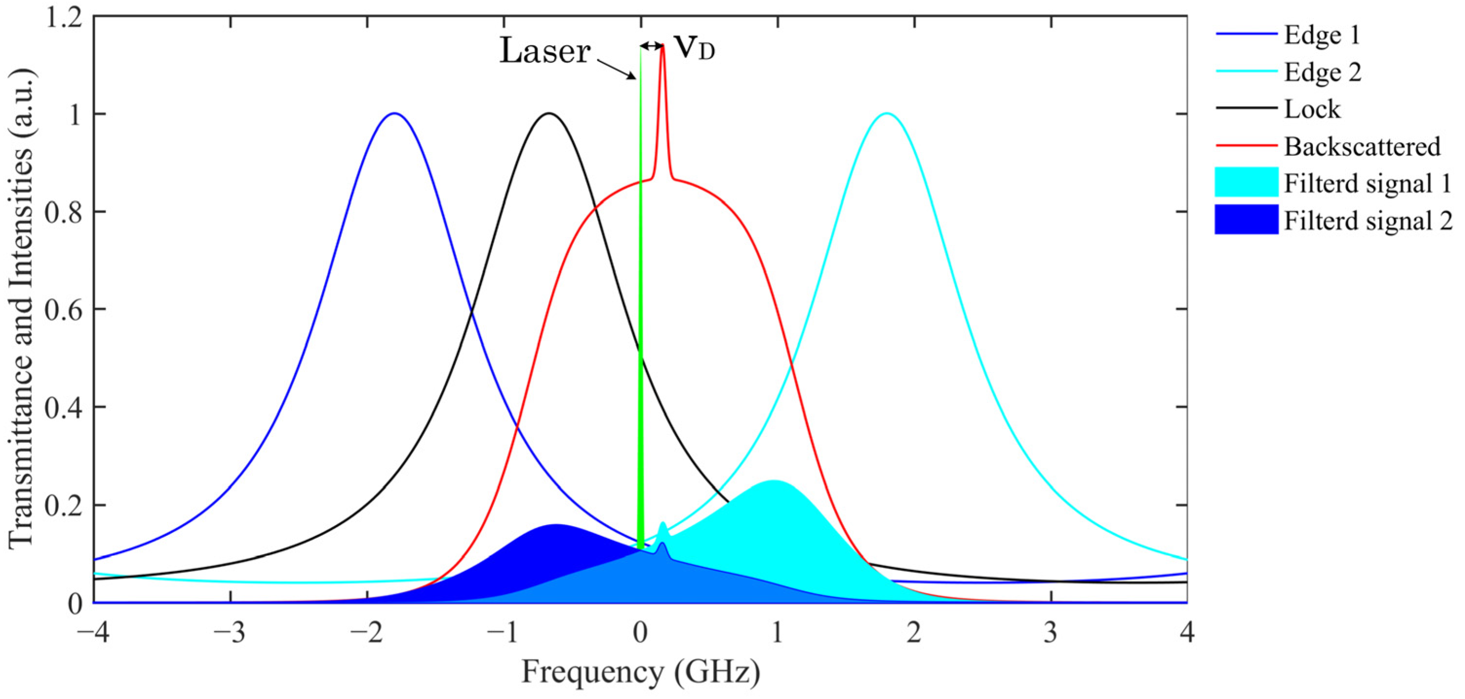
2.2. Double Edge Technique and FPI Frequency Identification

In general, most direct-detection wind LiDAR systems employ solid-state lasers that emit laser beams with narrow linewidth Gaussian spectral lines, and it is crucial to use an optical filter with a similarly steep spectral line. This enables the distinction of changes in spectral line transmittance, which can then be converted into Doppler shifts for wind measurement purposes. Currently, Fabry–Perot interferometers (FPI) are widely used for detecting atmospheric wind fields at middle and high altitudes. The rotary Rayleigh Doppler wind LiDAR (RRDWL) utilizes a double edge technology. This involves differentially processing the laser signal emitted by the laser as a reference signal with the atmospheric backscattered light signal received by the telescope. Figure 1 illustrates this concept.
The system utilizes a tunable FPI with an adjustable optical path between two plates. The FPI is divided into three channels, and the total aperture of the light-passing part is 80 mm. Two of the channels are dedicated to measuring the atmospheric echo signal, while the third channel is used for frequency locking, ensuring that the transmittance line of the FPI is aligned with the laser frequency. However, due to slight differences in film thickness, the optical path difference between the plates in each channel will vary slightly. As a result, the transmittance spectral lines of the three channels become independent of each other, allowing for a separate analysis and processing of their respective signals. In Figure 2, the principle of frequency discrimination using the FPI is illustrated. The blue and cyan lines represent the two edge channels, while the black lines represent the locked channel. The signal intensity in the edge channels is determined by the convolution of the atmospheric echo and the spectral response of the edge channels. The Doppler shift alters the relative position of the atmospheric backscattered spectrum, causing the signals in the edge channels to rise or fall accordingly. The green line in the middle represents the initial frequency of the emitted laser. The two blue areas represent the signal spectra after passing through the two edge channels, with the area representing the signal strength. In the absence of wind, when there is no Doppler shift, the signal spectra in the two edge channels are symmetric with each other. However, in the presence of wind, the atmospheric backscattered light signal experiences a Doppler frequency shift, resulting in changes in the signals of the two edge channels. By comparing the intensity changes between the emitted laser signal and the atmospheric backscattered light signal, the Doppler shift information can be derived. This information is then used to determine the radial wind speed at the corresponding height. Essentially, by using the FPI as a frequency discriminator, the radial wind speed can be obtained simply by analyzing the intensity changes in the two signals.

2.3. Wind Velocity Inversion and Synthesis

During actual wind field detection, the atmospheric echo signal passing through the FPI edge channel can be obtained by convolving the transmittance spectral lines of the two edge channels with the backscattered signal spectral lines of atmospheric molecules.
T R i ( v ) = h ( v ) f L ( v ) f R a y ( v ) ,
where f L v represents the spectral line of the emitted laser, h v represents the actual transmittance function of FPI, f R a y v represents the Rayleigh backscattering spectrum after the interaction of atmospheric molecules with the laser, i = 1 , 2 represents the two edge channels of FPI, and “ ” represents the convolution. According to the sum of the transmittance after the convolution of the two channels, the response curve of the system to the frequency shift can be calculated:
R V ( v d , T ) = T R 1 ( v 0 + v d , T ) / T R 2 ( v 0 + v d , T ) ,
where ν 0 and ν d are the system frequency and Doppler shift when there is no wind, respectively, and T is the atmospheric temperature.
To obtain the vertical profile of atmospheric horizontal wind speed, it is necessary to have measurements from at least three or more directions to synthesize the radial wind speeds. This is because the atmospheric wind field is three-dimensional, and the horizontal wind speed and direction vary spatially. By measuring wind speeds from multiple directions, information about the wind speed in different directions can be obtained, allowing for the construction of the wind speed distribution in the vertical profile of the atmosphere. Assuming that the vertical wind speed can be neglected compared to the horizontal wind speed, the radial wind speed can be considered as the radial projection of the horizontal wind field. By measuring the radial wind speed in each direction, it is possible to derive the horizontal wind speed and direction through vector synthesis. There are generally two methods for vector synthesis: the three-beam, fixed-point scanning method and the four-beam, fixed-point scanning method. Using these three wind speed components, the vertical profile of wind speed in space can be constructed. Figure 3 illustrates the principle diagram of the four-beam scanning of radial wind speed and the decomposition diagram of the wind field in the radial direction. The system described in this paper utilizes the four-beam, fixed-point scanning method to measure the radial wind speed in the east, west, south, and north directions, and the zenith angle is set to 22° during actual measurement. The horizontal wind speed is decomposed into three directions: east–west (X-axis), north–south (Y-axis), and vertical (Z-axis). This approach allows for an independent consideration of the variation of wind speed in different directions, enabling a more comprehensive description and analysis of the wind field characteristics in the atmosphere.
In summary, the atmospheric horizontal wind speed and direction can be expressed as:
V h = V x 2 + V y 2 θ = ar cos ( V y / V h ) V x 0 2 π ar cos ( V y / V h ) V x 0 ,

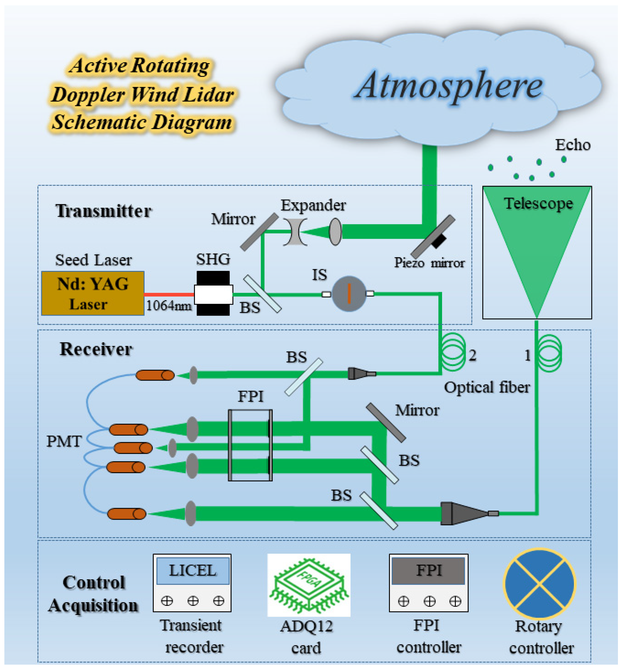
2.4. RRDWL System Parameters

The RRDWL consists of three key components: the transmitting optics, receiving optics, and control and acquisition subsystems, as shown in Figure 4. The transmitting optics subsystem comprises a seed injection Nd:YAG solid-state laser, a laser beam expander, and the emission light path. The seed injection Nd:YAG laser generates the laser pulse, while the laser beam expander enlarges the laser beam to the desired size. The laser light is then directed through the emission light path, passing through the emission mirror and into the atmosphere.
The receiving optics subsystem primarily consists of a Nessler Cassegrain receiving telescope, a receiving fiber, an FPI, a collimating device, a splitter path, interference filters, and a photomultiplier tube (PMT) among other key components. The receiving telescope captures the atmospheric backscattered light signal and focuses it onto the receiving fiber for transmission to the subsequent optical receiver. The collimating device ensures beam parallelism and stability. The echo light signal passes through the spectral light path and enters the FPI’s two edge channels. Interference filters are employed to select specific wavelength ranges according to the experimental requirements. Finally, the PMT is utilized for light signal collection.
The control and acquisition subsystem includes a transient recorder, such as Licel, a high-speed acquisition card, an industrial computer, and control inversion software. These components are responsible for controlling the system’s operation and parameter settings. Additionally, they facilitate the collection and processing of optical signal data.
By integrating these three subsystems, the system can effectively transmit the laser pulse into the atmosphere, receive the backscattered light signal, and control and acquire the optical data for further analysis and interpretation.

3. RRDWL Performance Test

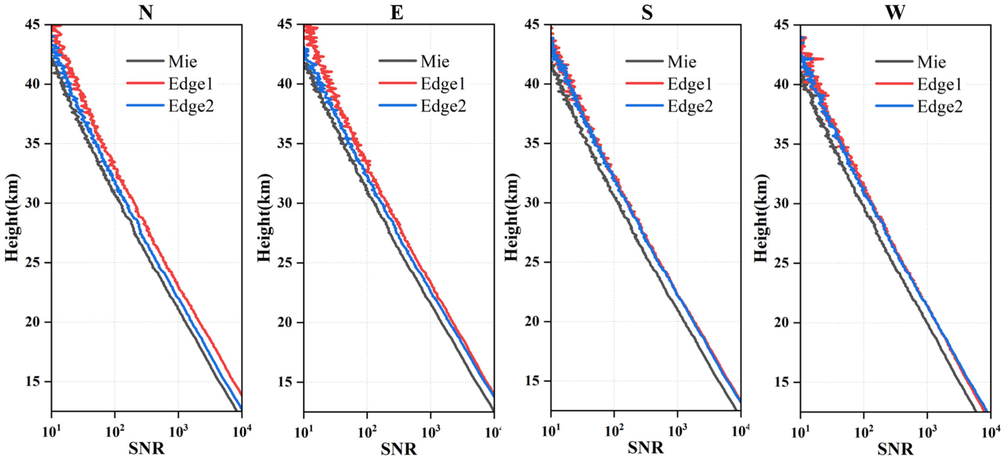
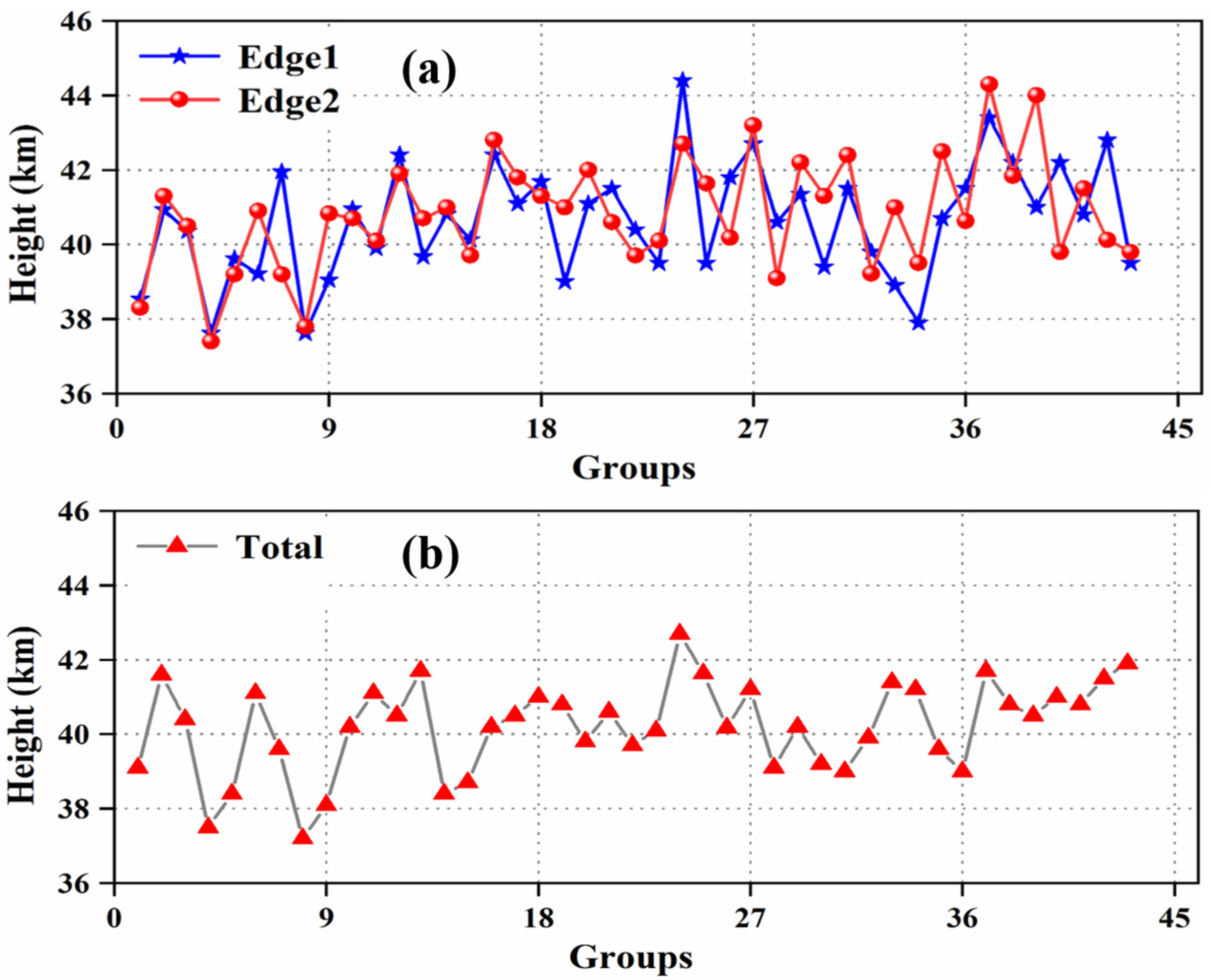
3.1. Performance Test Result

The RRDWL was completed in October 2021, as mentioned in Refs. [25,26] provide detailed information regarding the development and parameters of the system. Therefore, this article does not go into detail. Before the RRDWL can be deployed for atmospheric wind field observation missions, it is crucial to conduct field tests to comprehensively evaluate its detection performance. These tests are conducted to ensure that the system can operate reliably in real environments and provide accurate measurements of the wind field. For this purpose, the RRDWL was deployed on Science Island, located at coordinates 117.18° E and 31.47° N, in Hefei, Anhui Province. By conducting field tests in this area, the system’s capabilities can be thoroughly evaluated, and any necessary adjustments or optimizations can be made to ensure its effectiveness in practical wind field observations.
To mitigate the influence of complex weather conditions on the experimental results of the RRDWL system, the comparison observations between RRDWL and the Sonde wind field were conducted during the evening when the weather conditions were relatively favorable. It is important to acknowledge that the altitude region below 20 km in the troposphere is characterized by various weather phenomena and air turbulence. These factors can significantly amplify noise and pose challenges to the system’s ability to receive stable and reliable atmospheric echo signals effectively. At the same time, the pulse repetition rate of the main laser is 30 Hz, and RRDWL needs to complete four radial wind speed detections to obtain a horizontal wind field. Therefore, in order to ensure accurate measurements, the Rotational-Rate Dual-Wavelength LiDAR (RRDWL) emits a total of 8000 laser pulses in each direction during the detection process. This large number of pulses helps compensate for the potential noise and disturbances present in the lower troposphere. By carefully considering these factors and optimizing the system’s parameters, the RRDWL is able to acquire atmospheric wind field information in as little as 25 min. To enhance the signal-to-noise ratio of the system, spatial averaging processing was applied to the collected raw data, resulting in a range resolution of 300 m. In order to ensure the effective detection of atmospheric echo optical signals, the signal gate opening time delay after the completion of laser pulse Q-modulation was set to 80 microseconds. This configuration implies that the atmospheric echo optical signal profile becomes effective from a range of 11 km. Simultaneously, a weather balloon carrying a radiosonde was launched from the same location. The balloon reached an altitude of 28.01 km within 69 min, covering the entire operating time of the LiDAR system. According to GPS data, the balloon drifted 165.6 km to the east during its ascent.
In Figure 5a, the horizontal wind speed (WS) profiles obtained using the RRDWL and Sonde are depicted using black dots and red lines, respectively. In Figure 5b, the absolute deviation between the RRDWL and Sonde measurements is shown. It is observed that, except for a thin layer around 13 km and 18 km, the absolute deviation of the wind speed at other altitudes remains below 10 m/s. At a height of 12 km near the tropopause, the horizontal wind speed reaches a maximum of 90 m/s and then gradually decreases to within 5 m/s at an altitude of 22 km. Between 22 km and 27 km, a weak layer of wind is observed with peak winds of approximately 17 m/s. Overall, the comparison between the RRDWL and Sonde measurements shows reasonably good agreement, with the absolute deviation of wind speed mostly below 10 m/s, except for certain altitudes. In Figure 5c, the wind direction (WD) profile obtained using both the RRDWL and Sonde is presented. It can be observed that westerly winds, ranging from 227° to 292°, are prevalent at altitudes between 10 km and 27 km. This indicates a predominant westward flow in the atmosphere within this altitude range. At approximately 28 km, both the RRDWL and radiosonde measurements indicate the presence of wind shear. In Figure 5d, the deviation of wind direction between the RRDWL and Sonde measurements is shown. It is noteworthy that the deviation of wind direction between the RRDWL and Sonde measurements remains below 10° below 25 km. This suggests a relatively good agreement between the two devices in capturing the wind direction profile within this altitude range.

3.2. Measurement Error Analysis

During actual atmospheric wind field detection experiments, it is common for the detected data to deviate from theoretical simulation results due to measurement errors. These errors can be categorized into systematic errors and random errors, each contributing differently to the overall measurement accuracy and precision. Systematic errors are typically used to describe the accuracy of measurement results, representing consistent biases or offsets in the measurements. On the other hand, random errors are used to describe the precision of the measurements, reflecting variations or fluctuations in the measured values. The measurement accuracy, which quantitatively expresses the influence of both types of errors on the measurement results, can be characterized by uncertainty. The impact of these two types of errors on the measurement results is illustrated by the position distribution of red dots in Figure 6. Taking the small figure within Figure 5 as an example, Figure 6a indicates high measurement accuracy and small uncertainty, suggesting low systematic and random errors. In contrast, Figure 6d represents low measurement accuracy and large uncertainty, indicating significant systematic and random errors. Figure 6b demonstrates common errors encountered during detection, such as those caused by improper calibration coefficients. However, Figure 6c depicts the typical measurement errors of LiDAR, primarily dominated by random errors stemming from optical quantum noise and errors associated with system parameters. When both systematic and random errors are minimized, measurement results similar to those shown in Figure 6a can be obtained. The systematic errors of the RRDWL primarily arise from laser linewidth jitter, laser frequency jitter, system calibration, and inversion methods. These factors contribute to the overall systematic error in the measurements obtained using the system.
The signal-to-noise ratio (SNR) is a crucial metric widely used to assess the effective detection height in LiDAR systems. It quantifies the ratio of the desired signal strength to the level of background noise present in the received signal. In general, a higher signal intensity results in a higher SNR. SNR plays a significant role in determining the appropriate inversion height and calibration point in LiDAR systems. It directly influences the accuracy and reliability of the inversion results for atmospheric parameters. By selecting an inversion height with a higher SNR, the system can obtain more reliable and accurate measurements of atmospheric parameters. The formula to calculate SNR is typically defined as the ratio of the signal power to the noise power. However, the specific formulation can vary depending on the system and measurement configuration. It is essential to consider the characteristics and requirements of the LiDAR system in determining the appropriate SNR calculation method. Specifically, the SNR of RRDWL can be calculated as follows:
S N R ( z ) = N X ( z ) N X ( z ) + 2 ( N b + N d ) n ,
where NX (Z) is the atmospheric echo signal, Nb and Nd are the backscattered noise and atmospheric background radiation noise, and n is the pulse accumulation number.
In general, a region is considered valid if its signal-to-noise ratio (SNR) exceeds a predetermined threshold, such as 10. Consequently, a set of test data was selected to analyze the SNR profiles of the three channels of a four radial FPI. Figure 7 illustrates the results, indicating that the measured SNR is approximately 112 at a height of 30 km and around 10 at a height of 42 km. However, it is observed that the four radial signals gradually become unstable, starting from an altitude of 30 km, with the SNR exhibiting increasing jitter. It is important to note that, during actual measurements, several factors can cause inconsistencies in the SNR of different radials at the same height. These factors include the uneven distribution of the atmosphere and differences in the efficiency of the system’s detector components. Such variations can affect the strength of the signal and the level of noise, consequently resulting in disparities in the SNR values among different radials.
To evaluate the effective altitude of the system in long-term detection, an experiment was conducted wherein 8000 pulses were transmitted, and an SNR threshold of 10 was used as the evaluation criteria. The signals obtained during favorable atmospheric conditions were statistically analyzed, and the results are presented in Figure 8. In Figure 8a, the statistics for the effective detection heights of the two edge channels are displayed. It can be observed that edge channel 1 has a total of 17 sets of effective heights between 38 km and 40 km, and 26 sets between 40 km and 45 km. On the other hand, edge channel 2 has 12 sets with effective heights between 38 km and 40 km and 31 sets with effective heights between 40 km and 45 km. Figure 8b shows the statistical results of the combined effective detection altitudes. There are a total of 16 groups between 38 km and 40 km and 27 groups between 40 km and 43 km. In summary, the analysis indicates that the effective detection height of the RRDWL is primarily concentrated between 38 km and 42 km.
When using atmospheric backscatter signals with errors to invert atmospheric wind speed, the accuracy of the results can be affected by the transmission effect of the errors. The main source of measurement errors consists of random factors such as optical quantum noise, and it is closely associated with the technical parameters of the LiDAR system. During actual detection experiments, the presence of system errors can lead to the offset of the transmitting laser frequency from the intersection of the transmittance curve of the edge channel of the FPI. This offset can result in lower frequency locking accuracy. The wind speed error at this time is derived, and the frequency response function is:
R V = N 1 N 2 ,
where N1 and N2 indicate the edge channel transmittance of FPI. Through the error transfer function, the error in calculating radial wind speed is:
ε = 1 θ ( S / N ) ,
According to the mean square error of the actual frequency response function:
δ R V R V = ( 𝜕 ln R V 𝜕 N 1 δ N 1 ) 2 + ( 𝜕 ln R V 𝜕 N 2 δ N 2 ) 2 = ( δ N 1 N 1 ) 2 + ( δ N 2 N 2 ) 2 = ( 1 S N R 1 ) 2 + ( 1 S N R 2 ) 2 ,
Therefore, the actual wind speed error can be obtained according to the wind speed sensitivity and error transfer function:
θ V = 𝜕 R V / 𝜕 V R V ,
( δ R V R V ) 2 = ( 𝜕 ln R V 𝜕 V δ V ) 2 = ( θ V δ V ) 2 ,
𝜕 V = δ R V R V θ V = ( 1 S N R 1 ) 2 + ( 1 S N R 2 ) 2 θ V
To provide a more representative error analysis, another set of experimental data was utilized, and the random errors of the detected wind profiles were calculated using the aforementioned formula. The results are presented in Figure 9. In Figure 9a, the random errors of the four radial wind profiles in the east, south, west, and north directions are depicted. Figure 8b displays the random errors of the combined X and Y directions, as well as the horizontal wind speeds. According to the results shown in the figure, the random error of the wind profile exhibits an exponential increase with altitude. At 36 km, the four radial wind profiles demonstrate similar random error characteristics, with an approximate value of 10 m/s. The random error of the resulting horizontal wind speed is around 10 m/s at 34 km. The exponential growth of random errors with height emphasizes the importance of exercising caution when analyzing wind profile data at higher altitudes. Additionally, the similarity in random error characteristics among the four radial wind velocity profiles indicates consistency in data acquisition and processing. On the other hand, the random error of the synthesized horizontal wind velocity profile remains at a relatively high level. This finding underscores the need to fully consider the influence of random errors on the synthesis and inversion of horizontal wind velocities.
To provide a more intuitive comparison of the horizontal wind speed error profiles generated using the RRDWL, Figure 10 displays a diagram showcasing these profiles.
To compare the horizontal wind profiles obtained using the RRDWL and the Sonde, as well as the random error of wind speed calculated using SNR, Figure 11 provides a visual representation. In Figure 11a, the distribution trend of the horizontal wind speed profiles obtained using both devices is shown to be essentially the same. In Figure 11a, the distribution trend of the horizontal wind speed profiles obtained using both devices is shown to be essentially the same. The variation trend of the measured wind speed error and random error is similar to the height changes. This finding validates that the random error calculated using SNR can, to some extent, represent the wind measurement error and can be used to verify the accuracy of wind measurements. Furthermore, within the height range from 15 km to 25 km, significant jitter and large amplitude of the measured error can be observed. This suggests that system errors have a considerable impact on the accuracy of measurement results, in addition to the influence of atmospheric level heterogeneity. Figure 10 also highlights the significant effect of the zenith angle of the receiving telescope on the horizontal wind profile. Initially set at 22°, it was later found that setting the zenith angle to 24° resulted in better agreement between the RRDWL and radiosonde data. This indicates that the zenith angle plays an important role in the accuracy of measurement results. However, it is important to note that the zenith angle has less impact on the random error. Random errors are typically caused by various unpredictable factors, and the zenith angle mainly affects the measurement results based on system settings and instrument characteristics. The analysis results highlight the significant impact of system errors on the accuracy of measurement results, independent of atmospheric level heterogeneity. Additionally, the zenith angle of the receiving telescope is shown to have a notable effect on the accuracy of the horizontal wind profile. These findings emphasize that while the Rotary Rayleigh Doppler Wind Lidar (RRDWL) enables single-unit detection of the horizontal wind field, the presence of systematic errors can introduce significant inaccuracies in wind speed measurements.
To enhance the representativeness of the experimental results, statistical analysis was conducted on 35 sets of data obtained from successive detection experiments. Since the detection height of the Sonde does not typically exceed 30 km, the random error sequence of the wind speed in the horizontal wind profile at a height of 30 km, obtained from the RRDWL, was calculated and plotted in Figure 12. By examining Figure 11, it can be observed that the random error of the horizontal wind speed is below 10 m/s in 11 out of the 35 groups, while it exceeds 15 m/s in 5 out of the 35 groups. On average, the random error of the horizontal wind speed amounts to approximately 11.3 m/s. In summary, the effective detection height of the RRDWL system is primarily concentrated between 38 km and 42 km. Additionally, at an altitude of 30 km, the random error of the horizontal wind speed is approximately 11.3 m/s. Taking into account the statistical analysis of multiple experiments, these findings provide valuable insights into the performance and limitations of the RRDWL system. They contribute to understanding the effective detection range of the system and the expected level of random error in horizontal wind speed measurements at different altitudes.

4. Error Tracing Analysis

According to Section 3.2, the detection results of the RRDWL system are primarily influenced by two types of errors. The first type is a random error, primarily originating from light quantum noise. The second type of error arises from system-related factors, such as laser frequency jitter, operational stability, calibration, and inversion methods. Therefore, conducting traceability analysis to identify the main source of system error is crucial for optimizing the system’s performance. Considering that the RRDWL system utilizes a single unit for integral rotation, weighing nearly 6 tons, it is inevitable to encounter stability issues in the transceiver system during the actual detection process due to vibrations and structural deformations. These factors can significantly impact the overall detection performance. As depicted in Figure 13, on the evening of 13 March 2022, a continuous detection test was conducted by the system. Before the wind field detection experiment that night, a pre-experiment was carried out to observe the signal-to-noise ratio due to the cloudy weather, and no gating signal was set. The comparison diagram of atmospheric echo signals from three consecutive cycles in the north, east, south, and west (following the rotation sequence) reveals significant deviations within each group of four radial atmospheric echo signals over a short period of time (approximately 90 min), with varying change patterns. Based on this observation, it can be inferred that these deviations are caused by uneven ground conditions and that the deformation of the shelter is due to rotation, subsequently disrupting the collimation of the optical path in the transceiver subsystem.
In the emission subsystem, ensuring the stability of optical devices such as the fiber seed laser, main laser, and laser beam expander is crucial to maintaining the quality and frequency of the emitted laser beam. As stated, the equipment is in an open state during shelter operation, and it is inferred that the deformation of the resonator is primarily caused by changes in ambient temperature. To investigate this issue further, an ambient temperature test experiment was conducted in the afternoon of 19 January 2022, during winter, as shown in Figure 14. The purpose of this experiment was to assess the impact of ambient temperature on the resonator’s deformation. Initially, the main laser exhibited a fundamental frequency energy of approximately 1.5 J with a good pulse shape, indicating single longitudinal mode oscillation. After being turned off for four days, the factors causing changes in the main laser’s performance were investigated experimentally on January 24. Between 10:00 a.m. and 11:30 a.m., the equipment shelter was closed, and the main laser was preheated for 30 min. Despite the air conditioning being in heating mode, the 532 nm laser pulse exhibited a poor shape, showing a multi-longitudinal pattern, and the pulse energy was significantly reduced to around 300 mJ. This phenomenon was attributed to the change in ambient temperature. The room temperature at this time was 27 °C. Interestingly, when the air conditioner was turned off, the pulse shape improved, and the pulse energy was restored to about 620 mJ by adjusting the rear mirror. At 17:30 p.m., the main door of the equipment shelter was opened, causing the room temperature to rapidly drop from 27 °C to 20 °C. However, there were no significant changes observed in the pulse energy and waveform at this point, indicating that the cooling effect was not sufficient. To prolong the cooling time, the decision was made to close the hatch door. By 20:40 in the evening, the room temperature had reached 19 °C. Upon restarting the main laser, it was discovered that the energy of the fundamental amplification stage after seed injection had decreased to 0.74 J, while the energy of the 532 nm pulse had sharply dropped to 178 mJ. Subsequently, both the main and side doors of the equipment shelter were opened, causing the room temperature to rapidly decrease from 19 °C to 13 °C, allowing for the observation of the secondary effects of ambient temperature changes on the main laser. At this point, the energy of the 532 nm pulse was reduced to 160 mJ, and the pulse shape became highly chaotic, exhibiting a bimodal structure. At 21:10, the cabin door was closed, and the air conditioning was switched back to heating mode, causing the temperature to rise rapidly from 12 °C to 23 °C. However, the pulse energy of the oscillatory stage did not change significantly, and the waveform remained disordered. Efforts were made to strengthen the heating effect of the air conditioner, and, after working for more than half an hour, the room temperature was restored to 26 °C. However, the fundamental frequency oscillation stage energy after seed injection was only 107 mJ, indicating that the drastic change in ambient temperature had caused irreversible damage to the main laser and the seed injection process. As a result of this irreversible damage, the quality of the laser beam emitted could not be restored to normal levels.
This experimental investigation underscores the sensitivity of the main laser to ambient temperature changes and highlights the irreversible damage that can occur when subjected to rapid and extreme temperature fluctuations. Implementing measures to stabilize the ambient temperature and ensure gradual temperature transitions can help mitigate such issues and preserve the optimal performance of the main laser in the RRDWL system.
In the receiving subsystem, the stability of the optical receiver, particularly the successor optical receiver, is crucial. The transmittance curve of the FPI channel, which is incident upon by the beam, can be described using an Airy line, regardless of the beam’s divergence angle. This property offers significant advantages when measuring transmittance curves, as only a small number of points need to be measured to accurately fit the entire curve. By reducing the number of measurement points, the system can accumulate more laser pulses for each data point, thereby improving the signal-to-noise ratio. This enables more accurate measurements without requiring excessive scanning time. However, during the actual process of scanning the transmittance, it has been observed that when the beam has a divergence angle (which is usually unavoidable) and oblique incidence on the FPI, the transmittance curve becomes asymmetric. In such cases, accurately describing the transmittance curve using analytical formulas becomes challenging. To obtain an accurate spectral line of the FPI transmittance, a very small scanning step size is required to reduce the number of measured pulses at each point. Even with this measure, it takes nearly 40 min to accurately scan the entire FPI curve. Therefore, a good solution before scanning the transmittance curve of the FPI is to adjust the beam so that it is directly on the FPI without any divergence angle. However, in the early design of the receiver, the influence of the position and angle of the optical elements (such as filters, beam-splitting prisms, etc.) in the front and back optical paths of the FPI on mirror reflection was not fully considered. Additionally, due to vibrations caused by continuous rotation, the relative position of the optical elements inside the receiver may slightly change. The incomplete parallelism between the optical element and the surface of the FPI increases the degree of non-normal incidence of the beam. As a result, the detected signal contains components of oblique incidence through the FPI and surface reflection after the FPI, making it almost impossible to accurately describe the transmittance spectral line of the FPI using an analytical expression. Figure 15 displays the FPI transmittance spectral lines obtained from several rotation-detection experiments, along with the FPI transmittance spectral lines under ideal conditions. One can observe that, despite adjusting the incident beam to normal incidence, there remains a slight asymmetry in the spectral lines. However, after conducting numerous rotational detection tests, the spectral lines exhibit a significant increase in asymmetry. Upon inspecting the receiver, it was discovered that the root of the problem was the shift in the relative position of the mirror after the FPI, causing the incident light to reflect when passing through the filter in front of the photomultiplier tube (PMT). To address this issue, careful consideration should be given to the design of the receiver, taking into account the position and angle of the optical elements in relation to the FPI. Additionally, measures should be implemented to minimize vibrations and ensure the stability of the optical elements within the receiver. By addressing these factors, the accuracy of the transmittance measurements and the spectral line description of the FPI can be improved, leading to enhanced performance and reliability of the receiving subsystem.

5. Discussion

The atmospheric wind field data from the upper troposphere to the stratosphere (10–50 km) is of great significance for the in-depth study of the dynamics of the middle and upper atmosphere and the interaction between different layers. Compared with other detection methods, direct wind LiDAR has significant advantages in spatial resolution, detection range, and flexibility. At the same time, it is the only detection technology that can continuously and effectively obtain the high-precision data of three-dimensional wind fields in the troposphere and even the upper atmosphere.
Traditional direct wind LiDAR systems can be classified into two types. The first type is the scanning type, which incorporates a scanning mirror composed of two flat mirrors positioned above the LiDAR’s transmitter and receiver. This configuration enables the LiDAR system to detect the horizontal wind field by utilizing cone scanning. However, when the aperture of the receiving telescope exceeds half a meter, the size, thickness, and weight of the scanning mirror increase significantly. This not only poses challenges in terms of manufacturing complexity and cost but also makes optical tuning more difficult. Consequently, this method is only suitable for small and medium-sized systems, limiting the effective detection height of the system to the upper troposphere. Alternatively, researchers have employed a different approach to detect high-altitude wind fields by utilizing two (or three) large-aperture LiDAR systems arranged orthogonally (or at fixed angles) to measure different radial wind speeds. Typically, each system in this configuration has the same configuration and system parameters. By simultaneously measuring the line-of-sight wind speeds in different directions, it becomes possible to obtain the atmospheric level wind field at stratospheric and potentially higher altitudes. This detection method offers significant advantages, such as higher spatiotemporal resolution and an increased detection altitude range. However, it also presents certain challenges. Firstly, employing two or more subsystems necessitates the use of at least two high-power pulsed lasers, multiple large-aperture telescopes, and multiple detection and acquisition systems. This leads to increased development and maintenance costs while also raising the difficulty of precisely calibrating the instruments. Additionally, appropriate algorithms need to be employed to mitigate the impact of measurement discrepancies arising from errors in different subsystems. Since each subsystem may introduce varying sources of error, such as deviations in optical calibration or differences in detector response, these errors can potentially affect the final measurement results of the wind field. More importantly, whether it is a scanning system or a large aperture orthogonal system, the detection performance of direct wind LiDAR largely depends on the accuracy of the instrument. This includes factors such as the quality of the laser beam, the accuracy of the discriminator, and the response of the detector. The accuracy of these key parameters is crucial to obtain accurate and reliable wind field data. In addition, due to the need for larger telescopes and additional system configurations, the development cost of direct wind lidar is higher than that of coherent wind lidar. This means the direct wind LiDAR may be limited in practical applications. Another challenge is that different direct wind LiDAR systems use different discriminators and scanning modes, leading to differences in calibration methods. Calibration is an important step to ensure the measurement accuracy of the system. Different calibration methods may lead to inconsistencies between subsystems and limit the comparison and fusion of data.
In summary, the key factors that impact the performance of direct wind LiDAR can be further categorized as follows:
  • Laser Frequency Drift: Direct wind LiDAR systems typically use seed injection lasers, which can experience frequency drift due to temperature variations or vibrations. This drift can lead to significant errors in wind speed inversion.
  • Laser Beam Divergence and Stability: In real-world environments, the emitted laser beam may exhibit jitter or amplification in terms of divergence angle and frequency stability. This can impede the effective identification of Doppler frequency shifts caused by wind, resulting in increased errors in wind speed inversion. Suitable algorithms and devices are necessary to accurately identify and lock onto the frequency.
  • Instrument Stability and Calibration: Direct wind LiDAR systems often consist of multiple sets of precision instruments. The complex working environment can introduce varying degrees of error, impacting the stability and calibration of these instruments.
These factors collectively contribute to the slower research progress in direct wind LiDAR for detecting atmospheric wind fields. Additionally, it is worth noting that most field detections of direct wind LiDAR systems, both domestically and abroad, are primarily concentrated in high-latitude areas or regions with favorable meteorological conditions. This indicates that different meteorological conditions and complex external field environments present challenges for direct wind LiDAR, requiring further exploration and research.
Based on the above background, this research group has developed the first rotary Rayleigh Doppler wind LiDAR system in China. This innovative system utilizes a rotating platform structure to enable the detection of four radial wind speeds through integral rotation. The core components of the system include a seed injection laser, a large aperture receiving telescope, and a successor optical receiver. This design not only overcomes the limitation of traditional large aperture systems, which can only measure a single radial wind speed, but also enables a single direct wind measurement LiDAR system to detect the horizontal wind field in the middle and upper atmosphere. As a result, the system achieves a higher level of wind field detection compared to conventional approaches. Additionally, this design reduces the complexity of the structure and effectively lowers the development cost of the equipment. This development represents a significant advancement in direct wind LiDAR technology, offering improved capabilities for measuring wind speeds in different directions simultaneously. By utilizing the rotary Rayleigh Doppler wind detection LiDAR system, researchers can obtain comprehensive wind field data in the middle and upper atmosphere. This achievement holds promise for expanding the applications of direct wind LiDAR systems and advancing atmospheric research.

6. Conclusions

In order to effectively observe the stratospheric atmospheric wind field in the high troposphere, Xie et al. from the Chinese Academy of Sciences, Anhui Institute of Optics and Fine Mechanics (CAS, AIOFM) developed an innovative rotary Rayleigh Doppler wind measurement LiDAR (RRDWL). Following the completion of system construction, a performance test experiment was conducted to verify the feasibility of monomer detection of the atmospheric wind field in real-world environments. The results demonstrated that the system was capable of detecting the atmospheric wind field within an altitude range from 38 km to 42 km, with a horizontal wind speed error of approximately 11.3 m/s at 30 km altitude.
Furthermore, error analysis was performed to investigate the main factors influencing the system’s performance. It was identified that RRDWL had limitations in long-term continuous detection. The primary factor contributing to the reduction in effective detection height was the damage to optical axis parallelism caused by vibrations introduced by the rotating shelter and uneven ground surfaces. Additionally, random fluctuations in ambient temperature disrupted the seed laser injection process, thereby affecting the quality of the emitted beam. The imbalance in FPI parallelism resulting from non-normal incident beams and specular reflections had a significant impact on the accuracy of frequency discrimination. These error-tracing analyses provided valuable insights for optimizing the performance of RRDWL. Addressing the issues related to optical axis parallelism, vibration control, ambient temperature stability, seed laser injection, and FPI parallelism imbalance will be crucial for enhancing the system’s accuracy and reliability. Moreover, these findings serve as a foundation for the future long-term continuous supply of mid-upper atmospheric wind field data using RRDWL.

Author Contributions

Supervision, conceptualization, C.X.; resources, K.X.; software, B.W.; methodology, J.J. and L.L.; numerical simulation, writing—original draft preparation, J.C.; writing—review and editing, M.Z. All authors have read and agreed to the published version of the manuscript.

Funding

This work was supported in part by the Strategic Priority Research Program of the Chinese Academy of Sciences (XDA17040524), Anhui Province science and technology major project (201903c08020013).

Data Availability Statement

The data mentioned in the manuscript may be requested by email from the author.

Acknowledgments

I would like to thank the National Meteorological Center of China for the radiosonde data.

Conflicts of Interest

The authors declare no conflicts of interest.

References

  1. Yang, J.; Xiao, C.; Hu, X.; Xu, Q. Responses of zonal wind at ~40° N to stratospheric sudden warming events in the stratosphere, mesosphere and lower thermosphere. Sci. China Technol. Sci. 2017, 60, 935–945. [Google Scholar] [CrossRef]
  2. Zhao, R.; Dou, X.; Xue, X.; Sun, D.; Han, Y.; Chen, C.; Zheng, J.; Li, Z.; Zhou, A.; Han, Y.; et al. Stratosphere and lower mesosphere wind observation and gravity wave activities of the wind field in China using a mobile Rayleigh Doppler lidar. J. Geophys. Res. Space Phys. 2017, 122, 8847–8857. [Google Scholar] [CrossRef]
  3. Wang, Z.; Liu, Z.; Liu, L.; Wu, S.; Liu, B.; Li, Z.; Chu, X. Iodine-filter-based mobile Doppler lidar to make continuous and full-azimuth-scanned wind measurements: Data acquisition and analysis system, data retrieval methods, and error analysis. Appl. Opt. 2010, 49, 6960–6978. [Google Scholar] [CrossRef] [PubMed]
  4. Hedin, A.E.; Fleming, E.L.; Manson, A.H.; Schmidlin, F.J.; Avery, S.K.; Clark, R.R.; Franke, S.J.; Fraser, G.J.; Tsuda, T.; Vial, F.; et al. Empirical wind model for the upper, middle and lower atmosphere. J. Atmos. Terr. Phys. 1996, 58, 1421–1447. [Google Scholar] [CrossRef]
  5. Prasad, N.S.; Sibell, R.; Vetorino, S.; Higgins, R.; Tracy, A. All-Fiber, Modular, Compact Wind Lidar for Wind Sensing and Wake Vortex Applications. Proc. SPIE 2015, 9465, 94650C. [Google Scholar]
  6. Dou, X.; Han, Y.; Sun, D.; Xia, H.; Shu, Z.; Zhao, R.; Shangguan, M.; Guo, J. Mobile Rayleigh Doppler lidar for wind and temperature measurements in the stratosphere and lower mesosphere. Opt. Express 2014, 22, A1203–A1221. [Google Scholar] [CrossRef] [PubMed]
  7. Han, F.; Liu, H.; Sun, D.; Han, Y.; Zhou, A.; Zhang, N.; Chu, J.; Zheng, J.; Jiang, S.; Wang, Y. An Ultra-narrow Bandwidth Filter for Daytime Wind Measurement of Direct Detection Rayleigh Lidar. Curr. Opt. Photonics 2020, 4, 69–80. [Google Scholar]
  8. Lombard, L.; Valla, M.; Planchat, C.; Goular, D.; Augère, B.; Bourdon, P.; Canat, G. Eyesafe coherent detection wind lidar based on a beam-combined pulsed laser source. Opt. Lett. 2015, 40, 1030–1033. [Google Scholar] [CrossRef] [PubMed]
  9. Liu, H.; Zhu, X.; Fan, C.; Bi, D.; Liu, J.; Zhang, X.; Zhu, X.; Chen, W. Field Performance of All-Fiber Pulsed Coherent Doppler Lidar. Eur. Phys. J. Conf. 2020, 237, 08009. [Google Scholar] [CrossRef]
  10. Gentry, B.M.; Chen, H.; Li, S.X. Wind measurements with 355-nm molecular Doppler lidar. Opt. Lett. 2000, 25, 1231–1233. [Google Scholar] [CrossRef]
  11. Feifei, L.; Decang, B.; Heng, L.; Lucheng, Y.; Mingjian, W.; Xiaopeng, Z.; Jiqiao, L.; Weibiao, C. Principle Prototype and Experimental Progress of Wind Lidar in Near Space. Chin. J. Lasers 2020, 47, 0810003. [Google Scholar] [CrossRef]
  12. Souprayen, C.; Garnier, A.; Hertzog, A. Rayleigh-Mie Doppler wind lidar for atmospheric measurements. II. Mie scattering effect, theory, and calibration. Appl. Opt. 1999, 38, 2422–2431. [Google Scholar] [CrossRef] [PubMed]
  13. Chanin, M.L.; Garnier, A.; Hauchecorne, A.; Porteneuve, J. A doppler lidar for measuring winds in the middle atmosphere. Geophys. Res. Lett. 1989, 16, 1273–1276. [Google Scholar] [CrossRef]
  14. Baumgarten, G. Doppler Rayleigh/Mie/Raman lidar for wind and temperature measurements in the middle atmosphere up to 80 km. Atmos. Meas. Tech. 2010, 3, 1509–1518. [Google Scholar] [CrossRef]
  15. Huffaker, R.M.; Reveley, P.A. Solid-state coherent laser radar wind field measurement systems. Pure Appl. Opt. J. Eur. Opt. Soc. Part A 1998, 7, 863–873. [Google Scholar] [CrossRef]
  16. Zhao, Y.; Zhang, X.; Zhang, Y.; Ding, J.; Wang, K.; Gao, Y.; Su, R.; Fang, J. Data Processing and Analysis of Eight-Beam Wind Profile Coherent Wind Measurement Lidar. Remote Sens. 2021, 13, 3549. [Google Scholar] [CrossRef]
  17. Zhang, H.; Liu, X.; Wang, Q.; Zhang, J.; He, Z.; Zhang, X.; Li, R.; Zhang, K.; Tang, J.; Wu, S. Low-Level Wind Shear Identification along the Glide Path at BCIA by the Pulsed Coherent Doppler Lidar. Atmosphere 2020, 12, 50. [Google Scholar] [CrossRef]
  18. Guo, W.; Shen, F.; Shi, W.; Liu, M.; Wang, Y.; Zhu, C.; Shen, L.; Wang, B.; Zhuang, P. Data inversion method for dual-frequency Doppler lidar based on Fabry-Perot etalon quad-edge technique. Optik 2018, 159, 31–38. [Google Scholar] [CrossRef]
  19. Zhang, F. Research on Doppler Wind Lidar System with Wind Detection of High Temporal and Spatial Resolution. Ph.D. Thesis, University of Science and Technology of China, Hefei, China, 2015. (In Chinese). [Google Scholar]
  20. Shen, F.; Xie, C.; Qiu, C.; Wang, B. Fabry-Perot etalon-based ultraviolet trifrequency high-spectral-resolution lidar for wind, temperature, and aerosol measurements from 0.2 to 35 km altitude. Appl. Opt. 2018, 57, 9328–9340. [Google Scholar] [CrossRef]
  21. Xia, H.; Dou, X.; Shangguan, M.; Zhao, R.; Sun, D.; Wang, C.; Qiu, J.; Shu, Z.; Xue, X.; Han, Y.; et al. Stratospheric temperature measurement with scanningFabry-Perot interferometer for wind retrieval from mobile Rayleigh Doppler lidar. Opt. Express 2014, 22, 21775–21789. [Google Scholar] [CrossRef]
  22. Liu, Z.-S.; Wu, D.; Liu, J.-T.; Zhang, K.-L.; Chen, W.-B.; Song, X.-Q.; Hair, J.W.; She, C.-Y. Low-altitude atmospheric wind measurement from thecombined Mie and Rayleigh backscattering by Doppler lidar with an iodine filter. Appl. Opt. 2002, 41, 7079–7086. [Google Scholar] [CrossRef] [PubMed]
  23. Ansmann, A.; Ingmann, P.; Le Rille, O.; Lajas, D.; Wandinger, U. Particle backscatter and extinction profiling with the spaceborne HSR Doppler wind lidar ALADIN. Appl. Opt. 2007, 46, 6606–6622. [Google Scholar] [CrossRef] [PubMed]
  24. Zhang, C.; Sun, X.; Zhang, R.; Zhao, S.; Lu, W.; Liu, Y.; Fan, Z. Impact of solar background radiation on the accuracy of wind observations of spaceborne Doppler wind lidars based on their orbits and optical parameters. Opt. Express 2019, 27, A936–A952. [Google Scholar] [CrossRef] [PubMed]
  25. Zhao, M.; Xie, C.; Wang, B.; Xing, K.; Chen, J.; Fang, Z.; Li, L.; Cheng, L. A Rotary Platform Mounted Doppler Lidar for Wind Measurements in Upper Troposphere and Stratosphere. Remote Sens. 2022, 14, 5556. [Google Scholar] [CrossRef]
  26. Chen, J.; Xie, C.; Zhao, M.; Ji, J.; Wang, B.; Xing, K. Research on the Performance of an Active Rotating Tropospheric and Stratospheric Doppler Wind Lidar Transmitter and Receiver. Remote Sens. 2023, 15, 952. [Google Scholar] [CrossRef]
Figure 1. Double edge technology schematic diagram.
Photonics 11 00398 g001
Figure 2. Schematic diagram of FPI frequency discrimination principle.
Photonics 11 00398 g002
Figure 3. The principle diagram of radial wind speed was obtained using four-beam scanning.
Photonics 11 00398 g003
Figure 4. The principle diagram of RRDWL.
Photonics 11 00398 g004
Figure 5. Comparison of horizontal wind profiles obtained using RRDWL and Sonde. (a) wind speed (b) deviation of WS (c) wind direction (d) deviation of WD.
Photonics 11 00398 g005
Figure 6. Schematic diagram of random and systematic errors in measurement. (a) Small systematic error and random error (b) Large systematic error and small random error (c) Small systematic error and large random error (d) Both systematic error and random error are large.
Photonics 11 00398 g006
Figure 7. Four radial SNR profiles of a set of test data.
Photonics 11 00398 g007
Figure 8. Effective detection height sequence of RRDWL. (a) edge channel (b) system overall.
Photonics 11 00398 g008
Figure 9. Random error of wind speed at different altitudes (a) radial (b) synthesis.
Photonics 11 00398 g009
Figure 10. A set of horizontal wind speed error profiles for RRDWL.
Photonics 11 00398 g010
Figure 11. Horizontal wind field distribution under different zenith angles: (a) Wind profile comparison. (b) Measured error and random error.
Photonics 11 00398 g011
Figure 12. Continuous detection of 30 km horizontal wind speed error sequence.
Photonics 11 00398 g012
Figure 13. The change of four-radial atmospheric echo signal during continuous rotation.
Photonics 11 00398 g013
Figure 14. Main laser ambient temperature change curve.
Photonics 11 00398 g014
Figure 15. Influence of non-normal incidence and specular reflection of incident light on spectral lines of transmittance of FPI.
Photonics 11 00398 g015
Disclaimer/Publisher’s Note: The statements, opinions and data contained in all publications are solely those of the individual author(s) and contributor(s) and not of MDPI and/or the editor(s). MDPI and/or the editor(s) disclaim responsibility for any injury to people or property resulting from any ideas, methods, instructions or products referred to in the content.

