Online Denoising Single-Pixel Imaging Using Filtered Patterns

Abstract

Noise is inevitable in single-pixel imaging (SPI). Although post-processing algorithms can significantly improve image quality, they introduce additional processing time. To address this issue, we propose an online denoising single-pixel imaging scheme at the sampling stage, which uses the filter to optimize the illumination modulation patterns. The image is retrieved through the second-order correlation between the modulation patterns and the intensities detected by the single-pixel detector. Through simulations and experiments, we analyzed the impact of sampling rate, noise intensity, and filter template on the reconstructed images of both binary and grayscale objects. The results demonstrate that the denoising effect is comparable to the imaging-first followed by post-filtering procedures, but the post-processing time is reduced for the same image quality. This method offers a new way for rapid denoising in SPI, and it should be particularly advantageous in applications where time-saving is of paramount importance, such as in image-free large target classification.

1. Introduction

Single-pixel imaging (SPI) utilizes a spatial light modulator to generate a series of patterns to modulate the light field on an object, and the synchronized total intensities reflected or transmitted from the object are collected by a single-pixel detector. Through computing the second-order correlation, the two-dimensional or multi-dimensional information about the object can be recovered [1,2,3]. Compared with multi-pixel sensors, single-pixel detectors have the characteristics of low cost and superior durability. In recent years, SPI has been applied in various fields, such as remote sensing [4,5], hyperspectral imaging [6,7], X-ray imaging [8], terahertz imaging [9], and anti-interference imaging [10,11]. The emergence of compressed sensing [12], deep learning [13,14,15], and the improvement of computing power also accelerated the development of SPI. However, the applications mentioned above are subject to noise arising from source brightness fluctuations, environmental noise, and the detector’s electronic readout noise, resulting in decreased imaging quality. Thus, denoising has always been a challenge in SPI.

Researchers have proposed various schemes to improve the noisy image quality [16]. For example, differential ghost imaging [17,18] and normalized ghost imaging [19] are used to replace the traditional second-order correlation, and orthogonal modulation patterns have been proposed instead of random patterns to suppress the common mode noise. In addition, some post-processing algorithms have been proposed to improve imaging quality, such as iterative ghost imaging [20,21,22], compressed sensing [23], principal component analysis [24,25], convolutional neural networks [26,27], truncated singular value decomposition [28], and so on. There are also various hybrid denoising methods. In Reference [29], a two-step method combined with Tikhonov regularization and the U-Net network was designed to decrease the influence of noise. These post-processing algorithms can significantly suppress noise and improve imaging quality. However, denoising the sampled data directly still needs to be studied. The denoising of the sampling data will save post-processing time and give an advantage on image-free target classification or counting tasks.

This paper proposes a computationally efficient online denoising single-pixel imaging (ODSPI) scheme. It combines filtering with illumination patterns to achieve denoising during the sampling process. First, we demonstrated the feasibility of ODSPI theoretically. Then, we analyzed the effect of sampling rate, noise intensity, and filter template on the reconstructed image quality. The advantages of our approach in terms of time-saving were also discussed, and statistical analyses were conducted to verify the significance and reliability of ODSPI. Finally, the applicability of ODSPI was validated experimentally.

2. Theory

Single-pixel imaging can obtain an object’s two-dimensional or multi-dimensional information from the orthogonal illumination patterns and the correlated intensity measurements recorded by a single-pixel detector. The measurement $S_k$ is written as:

$$S_k={\displaystyle \sum _i^n{\displaystyle \sum _j^n{\phi }_{i,j}^k{x}_{i,j}}},$$

(1)

where ${\phi }^k\in {ℝ}^{n\times n}$ denotes the $k$-th illumination pattern, and $X\in {ℝ}^{n\times n}$ is the desired object scene. ${\phi }_{i,j}^k$ and $x_{i,j}$ represent the row i and column j values of the matrices ${\phi }^k$ and $x$, respectively. The object can be reconstructed from:

$$O=\frac{1}{M}{\displaystyle \sum _k^M{S}_k{\phi }^k},$$

(2)

where $O$ denotes the reconstructed image, and $M$ is the sampling number. In an experiment, some factors will introduce noise to the reconstructed image, such as the intensity fluctuation of the light source, the dark count of the detector, and the instability of the spatial light modulator. The object with noise is represented by $X_{noise}=X+\delta$, where $\delta$ represents the noise item. The noise type and level impact the choice of filter type and parameters. To improve the image quality without increasing the computational complexity of SPI, we used filtered illumination patterns to modulate the object. Assuming that $F$ is the filtering template, the filtered illumination pattern can be expressed as ${\phi }^{\prime }=\phi \otimes F$, where the symbol $\otimes$ represents convolution. It should be noted that the illumination patterns can be either random or orthogonal. Through the filtered patterns, we can directly obtain the filtered reconstructed image:

$$O={\displaystyle \sum _k^M\langle {\phi }^{k\prime }{x}_{noise}\rangle {\phi }^k},$$

(3)

where $\langle ·\rangle$ represents the inner product. According to the convolutional reciprocity theorem, Equation (3) also can be written as:

$$O={\displaystyle \sum _k^M\langle {\phi }^k{x}_{noise}\otimes F\rangle {\phi }^k}.$$

(4)

By comparing Equations (3) and (4), we can see that illumination pattern filtering and image filtering are equivalent in SPI. Thus, we were able to complete the image filtering during the sampling process. Based on this theory, we analyzed the effects of different filter templates, sampling rates, and noise intensities on the reconstructed image quality. Currently, the most commonly used filter templates are the mean filter, Gaussian low-pass filter, and Butterworth low-pass filter [30]. The formula for the mean filter is given by:

$${\overline{x}}_{i,j}=\frac{1}{m^2}{\displaystyle \sum _{i=1}^m{\displaystyle \sum _{j=1}^m{x}_{i,j}}},$$

(5)

where the window size of the mean filter is $m\times m$ pixels. $x_{i,j}$ represents the pixel value in row i and column j of the window, and ${\overline{x}}_{i,j}$ represents the average of all pixels in the window.

The kernel function of the Gaussian low-pass filter is expressed as follows:

$$G(x,y)={\mathrm{e}}^{\frac{-D^2(x,y)}{2D_0{}^2}},$$

(6)

where $D_0$ is the cutoff frequency and $D(x,y)$ is the distance from the pixel to the center in the window, and the window size of the Gaussian low-pass filter is the same as the mean filter.

The filter function of the Butterworth low-pass filter is

$$B(u,v)=\frac{1}{1+{(D(u,v)/D_0)}^{2\beta }},$$

(7)

where $\beta$ is the order of the filter, $D(u,v)$ denotes the distance from the pixel to the frequency’s origin, and $D_0$ represents the cutoff frequency of the filter.

In this paper, the peak signal-to-noise ratio (PSNR) and the root mean square error (RMSE) are applied to evaluate the quality of the reconstructed image, and are expressed as:

$$\begin{array}{l}PSNR=10\log \frac{Q^2}{\frac{1}{N}{\displaystyle \sum _{i=1,j=1}^n{(O(i,j)-X(i,j))}^2}}\\ RMSE=\sqrt{\frac{{\displaystyle \sum _{i=1,j=1}^n{(O(i,j)-X(i,j))}^2}}{N}}\end{array},$$

(8)

where N is the total pixel number of the object, $O(i,j)$ and $X(i,j)$ are the reconstructed and original images, respectively, and Q represents the maximum pixel value of the original image. When an 8-bit binary number represents the pixel value, the maximum Q is generally 255.

3. Numerical Simulation and Experiment Results

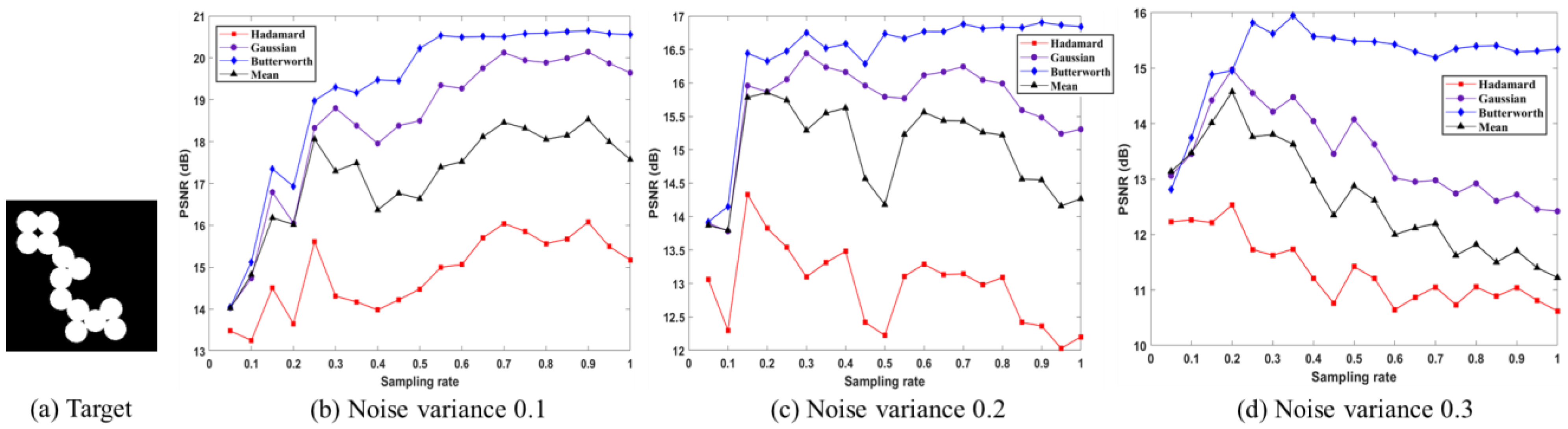
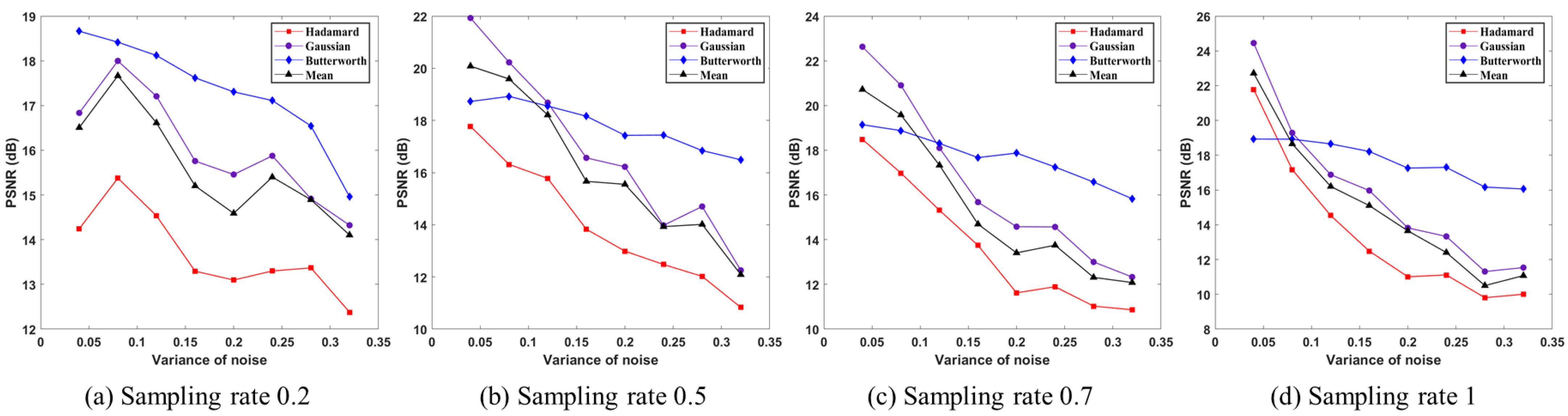
3.1. The Impacts of Sampling Rate, Noise Intensity, and Filtering Template on the Performance of ODSPI

To validate the performance of ODSPI, we compared the PSNR of the reconstructed objects of a binary object and a grayscale object under different sampling rates, noise intensities, and filtering templates. The original binary and grayscale objects are shown in Figure 1a and Figure 2a, respectively, with a resolution of 64 × 64 pixels. The filtering templates are the mean, Gaussian low-pass, and Butterworth low-pass filters. Assuming the light intensity is stable, the experimental noise generally follows a Gaussian distribution, so Gaussian noise was used in the simulation model.

Differential ghost imaging (DGI) is a fundamental reconstruction algorithm for SPI, and it is time-saving, so we chose it as the reconstruction algorithm in ODSPI. Additionally, we utilized the cake-cut sorted Hadamard basis [31] as the original illumination matrix. However, there is much freedom in choosing the original illumination patterns and reconstruction algorithm, and it will impact the performance of ODSPI. Reference [32] has demonstrated that the denoising efficacy of 3 $\times$ 3 pixels and 5 $\times$ 5 pixels filter templates are comparable, so we used 3 $\times$ 3 pixels as the window size for the mean and Gaussian low-pass filter templates. The cutoff frequency of the Gaussian low-pass filter was set to 0.8. In contrast, the Butterworth low-pass filter operates in the frequency domain, so the filter’s window size was set to 64 $\times$ 64 pixels and the cutoff frequency to 40.

The PSNR of binary and grayscale images under different sampling rates, noise variances, and filtering templates are shown in Figure 1, Figure 2, Figure 3 and Figure 4, where the red box indicates that the original Hadamard basis was used for the illumination patterns. At the same time, the black upper triangle, purple dots, and blue diamond represent the illumination patterns obtained by convolution of the Hadamard basis with the mean, Gaussian low-pass, and Butterworth low-pass filters, respectively.

Figure 1 and Figure 2 show the PSNR of binary and grayscale images under various sampling rates, with subfigures (b), (c), and (d) corresponding to noise variance of 0.1, 0.2, and 0.3, respectively. In Figure 1, we can see that the PSNRs obtained with ODSPI are consistently higher than that with the traditional SPI. The Butterworth low-pass filtered pattern demonstrates the best performance in suppressing noise, followed by the Gaussian low-pass and mean filters. In Figure 1b, as the sampling rate increases, the PSNR of the reconstructed objects shows an initial increase followed by stabilization. In Figure 1c,d, except for the Butterworth low-pass filtered pattern, the PSNR of the reconstructed objects for other filter patterns exhibits an initial increase followed by a decrease as the sampling rate increases. These phenomena are further validated in grayscale images, except for cases where noise variance is very low. In Figure 2b we can see that the PSNR obtained with the Gaussian low-pass filtered pattern is much higher than that of the Butterworth low-pass filtered pattern and Hadamard basis, while the PSNR of the mean filtered pattern is even worse than that of the Hadamard basis. We attribute these differences to the fixed parameter settings of the filters and the more high-frequency information in the grayscale images. Simulation results demonstrate that our scheme can effectively suppress noise for binary and grayscale images, except for the latter with low noise variance. Furthermore, as the noise intensity increases, the optimal sampling rate of ODSPI also varies between 0.2–0.6.

Figure 3 and Figure 4 show the PSNR of binary and grayscale objects under various noise variances, with subfigures (a), (b), (c), and (d) corresponding to sampling rates of 0.2, 0.5, 0.7, and 1, respectively. Figure 3 shows that the PSNR declines with the increase of noise variance for all illumination patterns. However, our scheme consistently achieved a higher PSNR for the reconstructed images compared to traditional SPI. The Butterworth low-pass filter gave the best performance as the noise variance increased, followed by the Gaussian low-pass and the mean-filtered pattern. When our scheme was applied to grayscale objects, it was not so advantageous under low noise intensity, but as the noise increased, noise suppression became more and more apparent, as shown in Figure 4. Overall, our scheme consistently outperformed traditional SPI in noise suppression for binary and grayscale images, except for the latter with low noise variance.

To further illustrate the performance of ODSPI, we present the reconstructed images of the “Circles” and “Peppers” with different sampling rates and illumination patterns for a noise variance of 0.1 in Figure 5 and Figure 6. The first to third rows represent the images reconstructed with 0.2, 0.5, and 0.7 sampling rates, respectively. The first to fourth columns show the images reconstructed with the original Hadamard basis, the mean filtered pattern, Gaussian low-pass filtered pattern, and Butterworth low-pass filtered pattern, respectively. The PSNRs are displayed below each reconstructed image. It can be observed that the image quality is consistent with the simulation results.

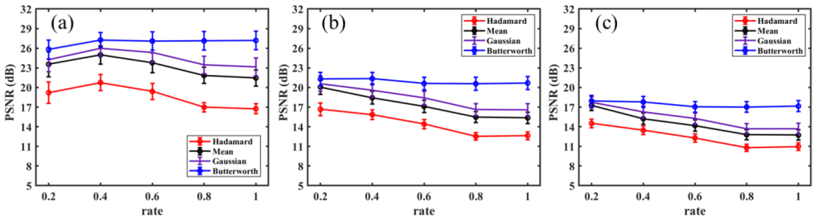
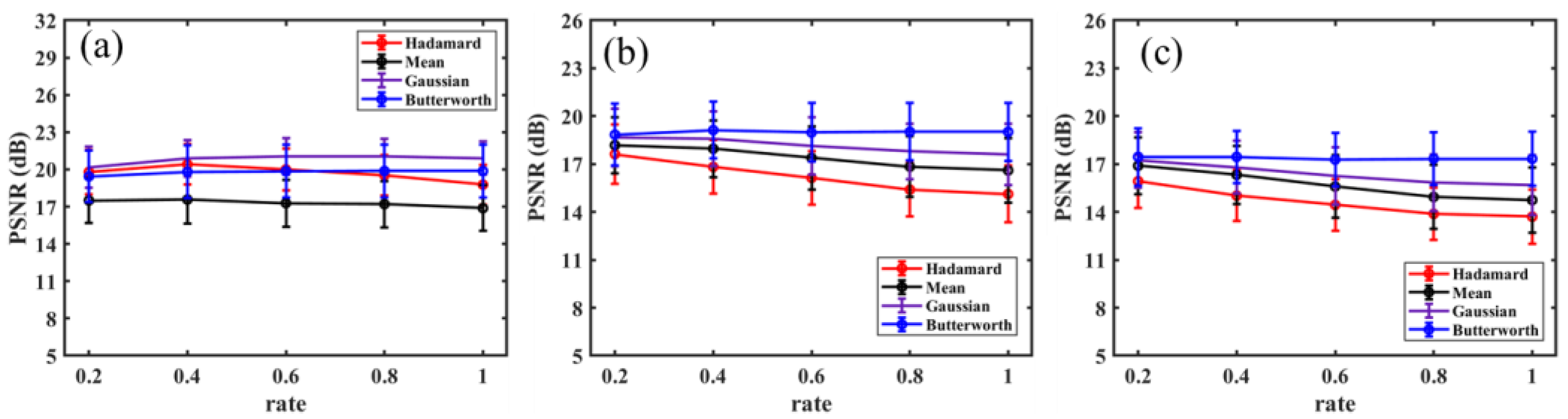
3.2. Time Advantage and Performance Analysis

When denoising the noisy image through filtering template, convolution is required. The number of convolutions mainly depends on the resolution of the image and can be calculated as follows:

$$Nc=\left(\left(S-K+2*P\right)/St+1\right)^2$$

(9)

where $Nc$ is the number of convolutions, $S$ the image size, $K$ the kernel size of the filter, $P$ the padding size of the image, and $St$ the stride size of the filter. Assuming a kernel size of 3, padding size of 0, and stride size of 1, an image with 256 $\times$ 256 pixels would require 64,516 convolution times, while an image with 512 $\times$ 512 pixels would require 260,100 convolutions. As the image’s resolution increases, the computation time required for denoising also increases. However, the proposed scheme in this study completed the denoising in the sampling stage, which saved the convolution time for the reconstructed images while maintaining the same quality as the image retrieved by post-processing.

To further validate the significance and reliability of ODSPI, we selected 40 binary images from the MNIST [33] and 40 grayscale images from STL-10 [34], then calculated the error bar of PSNR with traditional PSI and ODSPI under different sampling rates and noise variances. The images were resized to 64 × 64 pixels. The results are shown in Figure 7 and Figure 8, where the horizontal and vertical axes represent the sampling rate and PSNR. The subfigures, from left to right, are the reconstruction results for 0.1, 0.2, and 0.3 noise variances, respectively. Five sampling rates were chosen, namely 0.2, 0.4, 0.6, 0.8, and 1. The reconstruction algorithm was DGI, and the cake-cut sorted Hadamard basis served as the original illumination patterns.

Figure 7 shows the PSNRs obtained with binary images. We can see that the PSNRs of the filtered patterns are superior to those using the original pattern. The Butterworth low-pass filter achieved the best performance, followed by the Gaussian low-pass and mean filters. Figure 8 shows the PSNRs obtained with grayscale images. When the noise intensity was 0.1, as shown in Figure 8a, the Gaussian low-pass filter performed best; the mean filter performed poorly, while the Butterworth low-pass filtered pattern was nearly the same as that obtained with Hadamard basis. For noise variances of 0.2 and 0.3, as displayed in Figure 8b,c, the qualities of the reconstructed images with filtered patterns were superior to traditional SPI, and the Butterworth low-pass filter still achieved the best performance, followed by the Gaussian low-pass and mean filters. The standard deviation range of PSNRs for binary images was 0.56–1.9 dB, and for grayscale images was 1.36–2.14 dB. These results suggest that the performance of ODSPI on binary images is more stable than on grayscale images. Furthermore, our scheme exhibited outperformance on different binary and grayscale images, except for the latter with low noise variance. It demonstrated the significance and applicability of ODSPI.

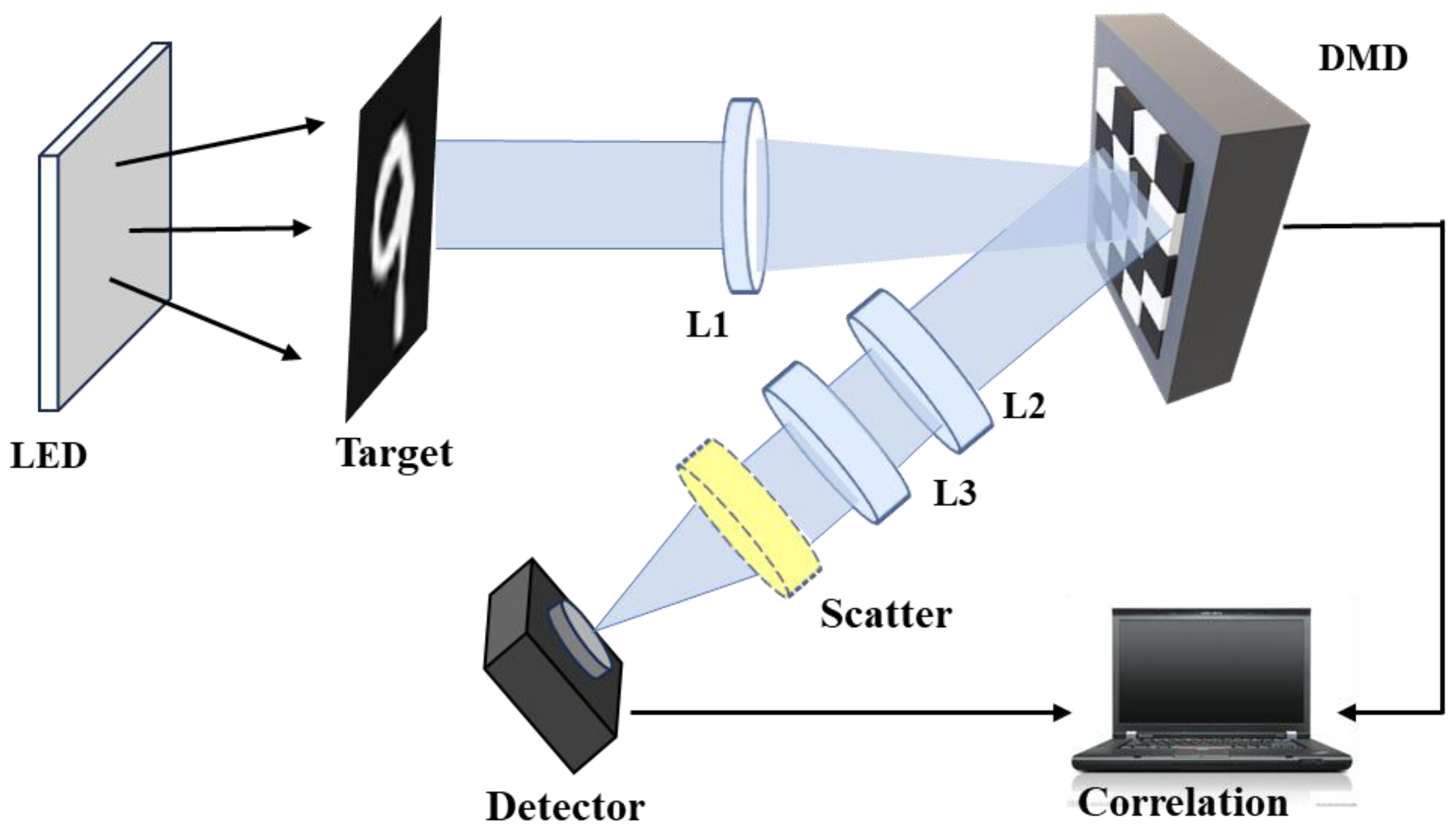
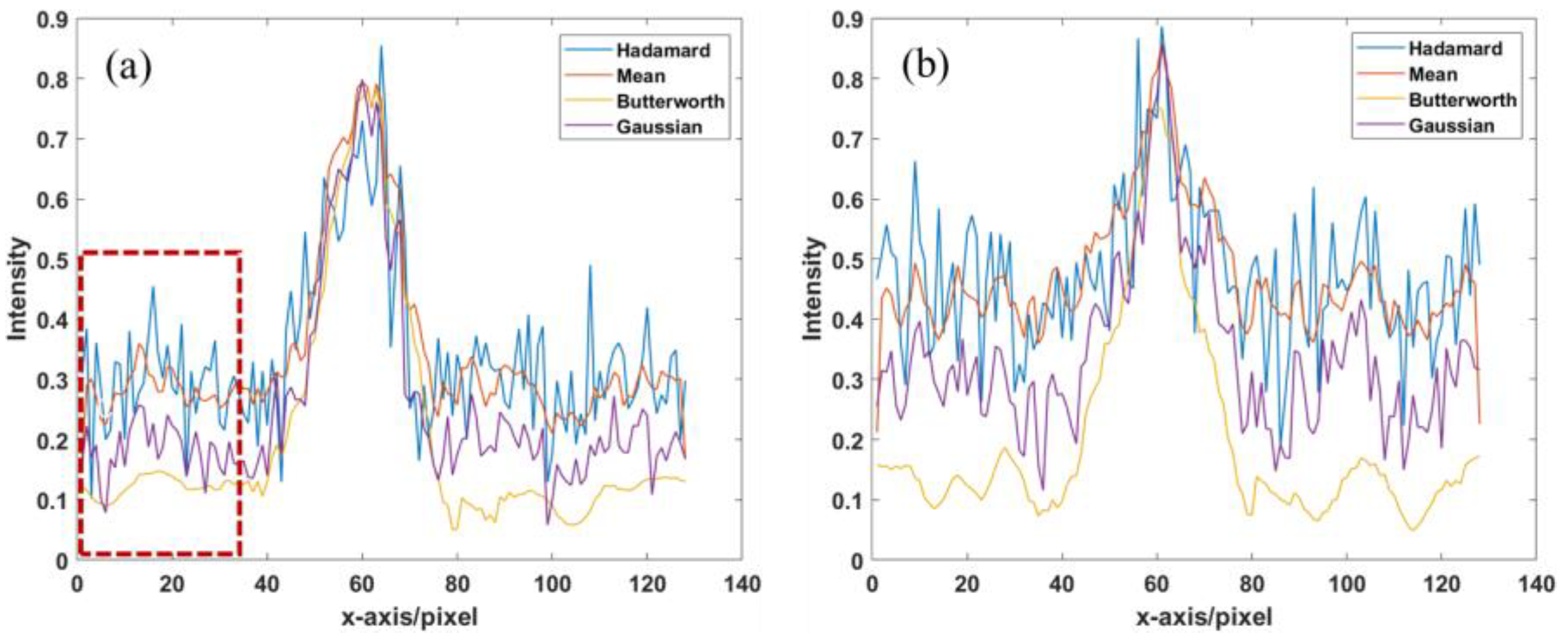
3.3. Experimental Results

The experimental setup for ODSPI is depicted in Figure 9. It comprises a light source, target object, digital micro-mirror device (DMD), single-pixel detector, data acquisition board, scattering plate, and lenses. We employed a light-emitting diode (LED) with an adjustable voltage range of 3–12 V for illumination. In the experiment, we set the voltage at 12 V. The target object was an 8 cm × 10 cm stencil plate etched with the digit “9”, carved out and placed in front of the LED. Lens L1 focused the transmitted light from the object onto the DMD (ViALUX, Karlsruhe, Germany, ViALUX-V7001, 1080 × 768 pixels), which was run at a refresh rate of 10 kHz. Each modulation pixel consisted of 6 $\times$ 6 binned micro-mirror pixels. Subsequently, converging lenses L1 and L2 collected the light reflected from the DMD and directed it toward the single-pixel detector (Thorlabs, Newton, NJ, USA, PDA100A2). The DMD was preloaded with patterns of 128 × 128 pixels generated by convolving the filter template with a Hadamard basis. Since the DMD can only load states of 1 and 0, but the filtered patterns were grayscale, the Floyd-Steinberg dithering algorithm [35] was employed to perform an appropriate conversion of the grayscale pattern to binary format before loading onto the DMD.

To verify the equivalence of the quality of the reconstructed object obtained through ODSPI and post-processing, we conducted comparison experiments, one using our ODSPI and the other post-filtering the reconstructed images. Guided by the simulation results, the sampling rate was set at 0.3. Thus, 4915 patterns were pre-loaded for each image. Figure 10 and Figure 11 show the reconstructed images. Additionally, each experiment compared the cases with and without a scattering plate before the single-pixel detector, as shown in Figure 9. The scatterer was a 1500 mesh B270 high borosilicate glass.

In Figure 10, the first and second rows represent the reconstructed objects without and with scattering plates, respectively. The four columns represent the reconstructed objects using the Hadamard basis, mean-filtered pattern, Gaussian low-pass filtered pattern, and Butterworth low-pass filtered pattern. The images obtained by post-filtering are shown in Figure 11, where again the first and second rows represent the filtered images without and with scattering, respectively. The first column shows the reconstructed objects with Hadamard basis, and the second to fourth columns show the results of filtering the reconstructed objects using the mean, Gaussian low-pass, and Butterworth low-pass filters, respectively. Comparing Figure 10 and Figure 11, we observe virtually no difference between their image qualities.

To evaluate the image quality more qualitatively, we plotted the intensities of the 77th row of Figure 10 and Figure 11 in Figure 12 and Figure 13, respectively. The position of the 77th row is indicated by the red line in Figure 10a. The blue, orange, purple, and yellow colors indicate illumination patterns using the Hadamard basis, the mean, Gaussian low-pass, and Butterworth low-pass filtered patterns, respectively. The left (a) and right (b) diagrams represent the reconstructed images without scattering and with scattering plates, respectively. We then calculated the RMSE of this row segment by choosing the first 34 pixels, as indicated by the red dashed box in Figure 12a. Since the position of the first 34 pixels was the background, which was non-transparent, the theoretical intensity value of the first 34 pixels should be 0.

The computed RMSE values are shown in

Table 1. Comparison of the RMSE of images reconstructed with ODSPI and post-filtering.

Filter Scheme	Noise Level	Hadamard	Mean	Gaussian	Butterworth
ODSPI	without scattering	0.303	0.283	0.174	0.124
	with scattering	0.46	0.425	0.285	0.136
Post-filtering	without scattering	0.303	0.276	0.192	0.103
	with scattering	0.46	0.387	0.2719	0.133

. We can see that filtering produced lower values than the unfiltered Hadamard patterns. When a scattering plate was inserted, the RMSE increased significantly, as would be expected. Furthermore, we find that ODSPI yielded closely identical RMSE values as post-filtering, demonstrating a comparable merit. It also shows a slight difference between the RMSE values with ODSPI and post-filtering. We attribute this to the fact that the experimental environment was not ideal. Nevertheless, the experiment results demonstrated the applicability of ODSPI.

4. Discussion

The chief advantage of ODSPI lies in its ability to filter data during the sampling stage, removing the time for post-processing. Additionally, when using the same reconstruction algorithm and sampling rate, our scheme produces similar image quality as post-filtering schemes. This feature is especially useful for large-size objects and has a particular advantage in image-free target classification or counting tasks [36].

However, there are certain limitations of ODSPI. Firstly, the performance of ODSPI is influenced by factors such as noise variance and type, so it is necessary to explore a method to estimate these parameters and adjust the sampling rate and filter parameters accordingly. Secondly, the low-pass filters employed in ODSPI are inadequate in preserving high-frequency information, resulting in blurry reconstructed images. The hybrid filter should be investigated to improve image quality and retain more high-frequency information. Thirdly, the imaging time and quality are related to the sampling number, and deep learning has gained widespread adoption in SPI for reducing the sampling rate. Thus, leveraging deep learning to improve image quality at lower sampling rates is viable.

5. Conclusions

In summary, we have introduced an online denoising scheme for SPI based on the convolutional reciprocity theorem, which generates denoised modulation patterns, facilitating image denoising during the sampling process, resulting in superior data quality and reducing the time required for post-processing. This temporal advantage will be significant for particular applications, such as image-free target recognition. Simulation and experiment results have demonstrated that ODSPI has better denoising performance than traditional SPI in binary and grayscale images, except for the latter with low noise variance. To further improve the performance of ODSPI in practical application, future investigations should focus on adaptively adjusting filter parameters and sampling rates according to noise type and variance. It is also valuable to utilize hybrid filters and non-linear reconstruction algorithms as alternatives to the current simplistic filters and reconstruction algorithms. These methods will further improve the image quality of ODSPI at lower sampling rates.

References

1. Pittman, T.B.; Shih, Y.H.; Strekalov, D.V.; Sergienko, A.V. Optical Imaging By Means of Two-Photon Quantum Entanglement. Phys. Rev. A 2002, 52, 3429–3432. [Google Scholar] [CrossRef] [PubMed]
2. Shapiro, J.H. Computational Ghost Imaging. Phys. Rev. A 2008, 78, 061802. [Google Scholar] [CrossRef]
3. Bennink, R.S.; Bentley, S.J.; Boyd, R.W. “Two-photon” Coincidence Imaging with a Classical Source. Phys. Rev. Lett. 2002, 89, 113601. [Google Scholar] [CrossRef] [PubMed]
4. Gong, W.L.; Zhao, C.Q.; Yu, H.; Chen, M.L.; Xu, W.D.; Han, S.S. Three-Dimensional Ghost Imaging Lidar via Sparsity Constraint. Sci. Rep. 2016, 6, 26133. [Google Scholar] [CrossRef] [PubMed]
5. Yu, W.K.; Liu, X.F.; Yao, X.R.; Wang, C.; Zhai, Y.; Zhai, G. Complementary Compressive Imaging for the Telescopic System. Sci. Rep. 2014, 4, 5834. [Google Scholar] [CrossRef]
6. Zhang, Z.B.; Liu, S.J.; Peng, J.Z.; Yao, M.H.; Zheng, G.A.; Zhong, J.G. Simultaneous Spatial, Spectral, and 3D Compressive Imaging via Efficient Fourier Single-Pixel Measurements. Optica 2018, 5, 315–319. [Google Scholar] [CrossRef]
7. Jin, S.J.; Hui, W.W.; Wang, Y.L.; Huang, K.C.; Shi, Q.S.; Ying, C.F.; Liu, D.Q.; Ye, Q.; Zhou, W.Y.; Tian, J.G. Hyperspectral Imaging Using the Single-Pixel Fourier Transform Technique. Sci. Rep. 2017, 7, 45209. [Google Scholar] [CrossRef]
8. Greenberg, J.; Krishnamurthy, K.; Brady, D. Compressive Single-Pixel Snapshot X-Ray Diffraction Imaging. Opt. Lett. 2014, 39, 111–114. [Google Scholar] [CrossRef]
9. Chan, W.L.; Charan, K.; Takhar, D.; Kelly, K.F.; Baraniuk, R.G.; Mittleman, D.M. A Single-Pixel Terahertz Imaging System Based on Compressed Sensing. Appl. Phys. Lett. 2008, 93, 121105. [Google Scholar] [CrossRef]
10. Durán, V.; Soldevila, F.; Irles, E.; Clemente, P.; Tajahuerce, E.; Andrés, P.; Lancis, J. Compressive Imaging in Scattering Media. Opt. Express 2015, 23, 14424–14433. [Google Scholar] [CrossRef]
11. Tajahuerce, E.; Durán, V.; Clemente, P.; Irles, E.; Soldevila, F.; Andrés, P.; Lancis, J.l. Image transmission through dynamic scattering media by single-pixel photodetection. Opt. Express 2014, 22, 16945–16955. [Google Scholar] [CrossRef] [PubMed]
12. Duarte, M.F.; Davenport, M.A.; Takhar, D.; Laska, J.N.; Sun, T.; Kelly, K.F.; Baraniuk, R.G. Single-pixel imaging via compressive sampling. IEEE Signal Process. Mag. 2008, 25, 83–91. [Google Scholar] [CrossRef]
13. Barbastathis, G.; Ozcan, A.; Situ, G. On the use of deep learning for computational imaging. Optica 2019, 6, 921–943. [Google Scholar] [CrossRef]
14. Wang, F.; Wang, H.; Wang, H.C.; Li, G.W.; Situ, G.H. Learning from simulation: An end-to-end deep-learning approach for computational ghost imaging. Opt. Express 2019, 27, 25560–25572. [Google Scholar] [CrossRef] [PubMed]
15. Jiao, S.M.; Feng, J.; Gao, Y.; Lei, T.; Xie, Z.W.; Yuan, X. COptical machine learning with incoherent light and a single-pixel detector. Opt. Lett. 2019, 44, 5186–5189. [Google Scholar] [CrossRef] [PubMed]
16. Yang, Z.H.; Sun, Y.Z.; Yan, R.T.; Qu, S.F.; Yu, Y.J.; Zhang, A.X.; Wu, L.A. Noise reduction in computational ghost imaging by interpolated monitoring. Appl. Opt. 2018, 12, 143–159. [Google Scholar] [CrossRef] [PubMed]
17. Ferri, F.; Magatti, D.; Lugiato, L.A.; Gatti, A. Differential Ghost Imaging. Phys. Rev. Lett. 2010, 104, 253603. [Google Scholar] [CrossRef]
18. Li, M.F.; Zhang, Y.R.; Luo, K.H.; Wu, L.A.; Fan, H. Time-Correspondence Differential Ghost Imaging. Phys. Rev. A 2013, 87, 033813. [Google Scholar] [CrossRef]
19. Sun, B.Q.; Welsh, S.S.; Edgar, M.P.; Shapiro, J.H.; Padgett, M.J. Normalized Ghost Imaging. Opt. Express 2012, 20, 16892. [Google Scholar] [CrossRef]
20. Yao, X.R.; Yu, W.K.; Liu, X.F.; Li, L.Z.; Li, M.F.; Wu, L.A.; Zhai, G.J. Iterative denoising of ghost imaging. Opt. Express 2014, 22, 24268–24275. [Google Scholar] [CrossRef]
21. Wang, W.; Wang, Y.P.; Li, J.; Yang, X.; Wu, Y. Iterative ghost imaging. Opt. Lett. 2014, 39, 5150. [Google Scholar] [CrossRef] [PubMed]
22. Zhou, Y.; Zhang, H.W.; Zhong, F.; Guo, S.X. Iterative denoising of ghost imaging based on adaptive threshold method. Acta Phys. Sin. 2018, 67, 244201. [Google Scholar] [CrossRef]
23. Du, J.; Gong, W.; Han, S. The influence of sparsity property of images on ghost imaging with thermal light. Opt. Lett. 2012, 37, 1067–1069. [Google Scholar] [CrossRef] [PubMed]
24. Wang, G.; Zheng, H.; Wang, W.; He, Y.; Liu, J.; Chen, H.; Xu, Z. Denoising ghost imaging via principal components analysis and compandor. Opt. Lasers Eng. 2018, 110, 236–243. [Google Scholar] [CrossRef]
25. Guan, Q.; Deng, H.; Gao, X.; Zhong, X.; Ma, M.; Gong, X. Source separation and noise reduction in single-pixel imaging. Opt. Lasers Eng. 2023, 170, 107773. [Google Scholar] [CrossRef]
26. Wu, H.; Wang, R.; Zhao, G.; Xiao, H.; Liang, J.; Wang, D.; Tian, X.B.; Cheng, L.L.; Zhang, X.M. Deep-learning denoising computational ghost imaging. Opt. Lasers Eng. 2020, 134, 106183. [Google Scholar] [CrossRef]
27. Hu, H.K.; Sun, S.; Lin, H.Z.; Jiang, L.; Liu, W.T. Denoising ghost imaging under a small sampling rate via deep learning for tracking and imaging moving objects. Opt. Express 2020, 28, 37284–37293. [Google Scholar] [CrossRef]
28. Chen, L.Y.; Wang, C.; Xiao, X.Y.; Ren, C.; Zhang, D.J.; Li, Z.; Cao, D.Z. Denoising in SVD-based ghost imaging. Opt. Express 2022, 30, 6248–6257. [Google Scholar] [CrossRef]
29. Pronina, V.; Mur, A.L.; Abascal, J.F.; Peyrin, F.; Dylov, D.V.; Ducros, N. 3D denoised completion network for deep single-pixel reconstruction of hyperspectral images. Opt. Express 2021, 29, 39559–39573. [Google Scholar] [CrossRef]
30. Gonzalez, R.C.; Woods, R.E. Digital Image Processing, 3rd ed.; Prentice Hall: Upper Saddle River, NJ, USA, 2008; pp. 291–308. [Google Scholar]
31. Yu, W.K. Super sub-Nyquist single-pixel imaging by means of cake-cutting Hadamard basis sort. Sensors 2019, 19, 4122. [Google Scholar] [CrossRef]
32. Zhen, J.H.; Yu, X.D.; Zhao, S.M.; Wang, L. Ghost Imaging Denoising Based on Mean Filtering. Acta Opt. Sin. 2022, 42, 2211002. [Google Scholar]
33. LeCun, Y.; Cortes, C.; Burges, C. MNIST Handwritten Digit Database. AT&T Labs. 2010. Available online: http://yann.lecun.com/exdb/mnist (accessed on 30 May 2018).
34. Coates, A.; Ng, A.; Lee, H. An analysis of single-layer networks in unsupervised feature learning. In Proceedings of the Fourteenth International Conference on Artificial Intelligence and Statistics, Fort Lauderdale, FL, USA, 11–13 April 2011. [Google Scholar]
35. Zhang, Z.B.; Wang, X.Y.; Zheng, G.A.; Zhong, J.G. Fast Fourier single-pixel imaging via binary illumination. Sci. Rep. 2017, 7, 12029. [Google Scholar] [CrossRef] [PubMed]
36. Ota, S.; Horisaki, R.; Kawamura, Y.; Ugawa, M.; Sato, I.; Hashimoto, K.; Noji, H. Ghost cytometry. Science 2018, 360, 1246–1251. [Google Scholar] [CrossRef] [PubMed]
Figure 1. PSNR of “Circles” reconstructed at different sampling rates. (a) is the original object, (b), (c), and (d) represent the PSNR of the reconstructed images with noise variances of 0.1, 0.2, and 0.3, respectively.
Photonics 11 00059 g001
Figure 2. PSNR of “Peppers” reconstructed at different sampling rates. (a) is the original object, (b), (c), and (d) represent the PSNR of the reconstructed images with noise variances of 0.1, 0.2, and 0.3, respectively.
Photonics 11 00059 g002
Figure 3. PSNR of “Circles” reconstructed at different noise variances. (a), (b), (c), and (d) represent the PSNR of the reconstructed images with sampling rates of 0.2, 0.5, 0.7, and 1, respectively.
Photonics 11 00059 g003
Figure 4. PSNR of “Peppers” was reconstructed at different noise variances. (a), (b), (c), and (d) represent the PSNR of the reconstructed images with sampling rates of 0.2, 0.5, 0.7, and 1, respectively.
Photonics 11 00059 g004
Figure 5. Reconstructed images of “Circles” with traditional SPI and ODSPI at different sampling rates and modulation patterns. The PSNR are presented below each image.
Photonics 11 00059 g005
Figure 6. Reconstructed images of “Peppers” with traditional SPI and ODSPI at different sampling rates and modulation patterns. The PSNR are presented below each image.
Photonics 11 00059 g006
Figure 7. The PSNRs obtained with 40 binary objects from the MNIST dataset, where (a), (b), and (c) correspond to the PSNRs under noise variances of 0.1, 0.2, and 0.3, respectively.
Photonics 11 00059 g007
Figure 8. The PSNRs obtained with 40 grayscale objects from the STL-10 dataset, where (a), (b), and (c) correspond to the PSNRs under noise variances of 0.1, 0.2, and 0.3, respectively.
Photonics 11 00059 g008
Figure 9. Schematic of online denoising single-pixel imaging.
Photonics 11 00059 g009
Figure 10. Images reconstructed with ODSPI. The first to fourth columns represent images obtained with the Hadamard basis, mean-filtered pattern, Gaussian low-pass filtered pattern, and Butterworth low-pass filtered pattern, respectively. The red line in (a) represents the position of the 77th row. (ad) and (ef) depict the images obtained without and with the addition of a scattering plate, respectively.
Photonics 11 00059 g010
Figure 11. Images obtained by post-filtering. (a,e) show the reconstructed objects with Hadamard basis. and the second to fourth columns show the results of filtering the reconstructed objects using the mean, Gaussian low-pass, and Butterworth low-pass filters, respectively. (ad) and (e,f) depict the images obtained without and with the addition of a scattering plate, respectively.
Photonics 11 00059 g011
Figure 12. Intensity values extracted from the 77th row of Figure 10. (a) Without scattering. (b) With scattering. The red dashed box indicates the position of the first 34 pixels of the 77th row.
Photonics 11 00059 g012
Figure 13. Intensity values extracted from the 77th row of Figure 11. (a) Without scattering. (b) With scattering.
Photonics 11 00059 g013