A Parabolic Waveform Generator Based on the Chirp Characteristics of a Directly Modulated Laser

Abstract

Due to carrier dynamics, the modulated light field from a directly modulated laser (DML) has an intensity envelope with a certain frequency chirp. When the chirp is linearly mapped into intensity by a frequency discriminator such as an optical filter with a linear edge, the optical field presents a new signal determined by the multiplication operation between the envelope function and the chirp function. Under a triangular drive signal, this process can contribute dark, bright and frequency-doubled bright parabolic waveforms by properly adjusting the filter window. This method is verified by both a theoretical analysis and experimental demonstrations. It not only provides a low-cost and simple scheme to generate parabola signals, but also a new method for arbitrary waveform generation.

1. Introduction

Linear chirp generation in an optical field has widespread applications, such as optical pulse compression [1] and temporal Fourier processing based on time lenses [2,3,4]. Since the chirp is the time derivative of the phase, a linear chirp can be achieved via electro-optic phase modulation with parabolic drive signals or cross-phase modulation with a parabolic pump pulse in nonlinear elements [5,6]. Therefore, parabolic waveform generation consequently has attracted considerable attention.

Many schemes for parabolic pulse generation have been reported in recent decades. One method is implemented by the envelope revolution through propagation in optical fibers. This scheme takes advantage of the self-similar propagation of short pulses, in which a pulse with a parabolic intensity profile propagates in fibers with normal group-velocity dispersion (GVD) and strong nonlinearity. However, this process is greatly limited by third-order dispersion and the fiber parameters needs to be precisely controlled [7,8]. Another scheme involves generating bright and dark parabolic pulses through an array waveguide. In this method, the intensity and phase of each harmonic component of an optical short pulse are manipulated line-by-line in the spectral domain, finally synthesizing a parabolic pulse in the time domain because of the mapping relationship from the frequency domain to the time domain. However, the stability and complexity limit its application [9]. Some schemes for parabolic pulse generation based on the Mach–Zehnder modulator (MZM) are also reported. One proposal is that a Gaussian pulse is stretched to realize the wavelength-to-time mapping, and the mapped signal is modulated by an MZM with an appropriately designed drive signal to obtain a parabolic pulse [10]. In addition, the modulation characteristics of MZMs can also be utilized for parabolic pulse generation. In this case, the transmission curve of an MZM can be mapped into the time domain by applying a drive signal with a linear edge, e.g., a triangular pulse, which eventually outputs a parabolic pulse because the peak or valley of the transmission curve of an MZM approaches a parabolic function [11]. In order to generate accurate parabolic pulses, a simple scheme for parabolic pulse generation is demonstrated, in which a parabola can be expressed as a quadratic function and consequently implemented by the product of two linear functions. Although this method is mathematically intuitionistic, the system is relatively complicated because of the cascade of multiple modulators [12]. In [13], an approach for parabolic pulse generation based on an optical fiber loop mirror is proposed and experimentally demonstrated. This approach is able to flexibly achieve a higher operation bandwidth, such as parabolic pulse generation with repetition frequencies of 8, 9 and 10 GHz. However, due to the use of a non-reciprocal Sagnac interferometer and a highly nonlinear fiber (HNLF), the polarization stability of the system and power requirements are relatively high.

In this paper, a simpler parabolic waveform generator based on the chirp characteristics of a DML is proposed. The desired chirp signal can be obtained by the carrier dynamics of a DML under a triangular drive signal. By setting the modulation depth appropriately, the chirped signal can be linearly mapped into the time domain via an optical filter with a linear edge. Finally, the mapped signal is spontaneously multiplied by the envelope function of the modulated signal to successfully generate a dark, bright parabolic pulse and a frequency-doubled bright pulse, which agrees with the theoretical expectation well.

2. Operation Principle

Theoretically, when a DML is driven by an electrical pulse $p\left(t\right)$, an optical signal with an intensity of $p\left(t\right)$ with a chirp of $△v\left(t\right)$ will be output. The chirp of the output light field is given in [14]

$$△v\left(t\right)\approx -\frac{\alpha }{4\pi }\left\{\frac{d}{dt}ln\left[p\left(t\right)\right]+\kappa p\left(t\right)\right\},$$

(1)

where $\alpha$ is the line-width enhancement factor of the laser, $p\left(t\right)$ is the envelope of drive signal and $\kappa =2\Gamma \epsilon /V_{act}\eta h\omega$ is the adiabatic chirp coefficient. In the expression of $\kappa$, $\Gamma$ is the optical confinement factor, $\epsilon$ is the gain saturation factor of the laser, $V_{act}$ is the volume of the active region, $\eta$ is the differential quantum efficiency, h is the Planck constant and $\omega$ is the optical angular frequency. Since all of the parameters are fixed for a certain DML, $\kappa$ is a constant. In Equation (1), the first term denotes the transient chirp and the second term represents the adiabatic chirp. When the laser bias current is much larger than the threshold, the transient chirp term can be neglected and the total chirp can be simplified to [15]

$$△v\left(t\right)=-\frac{\alpha \kappa }{4\pi }p\left(t\right).$$

(2)

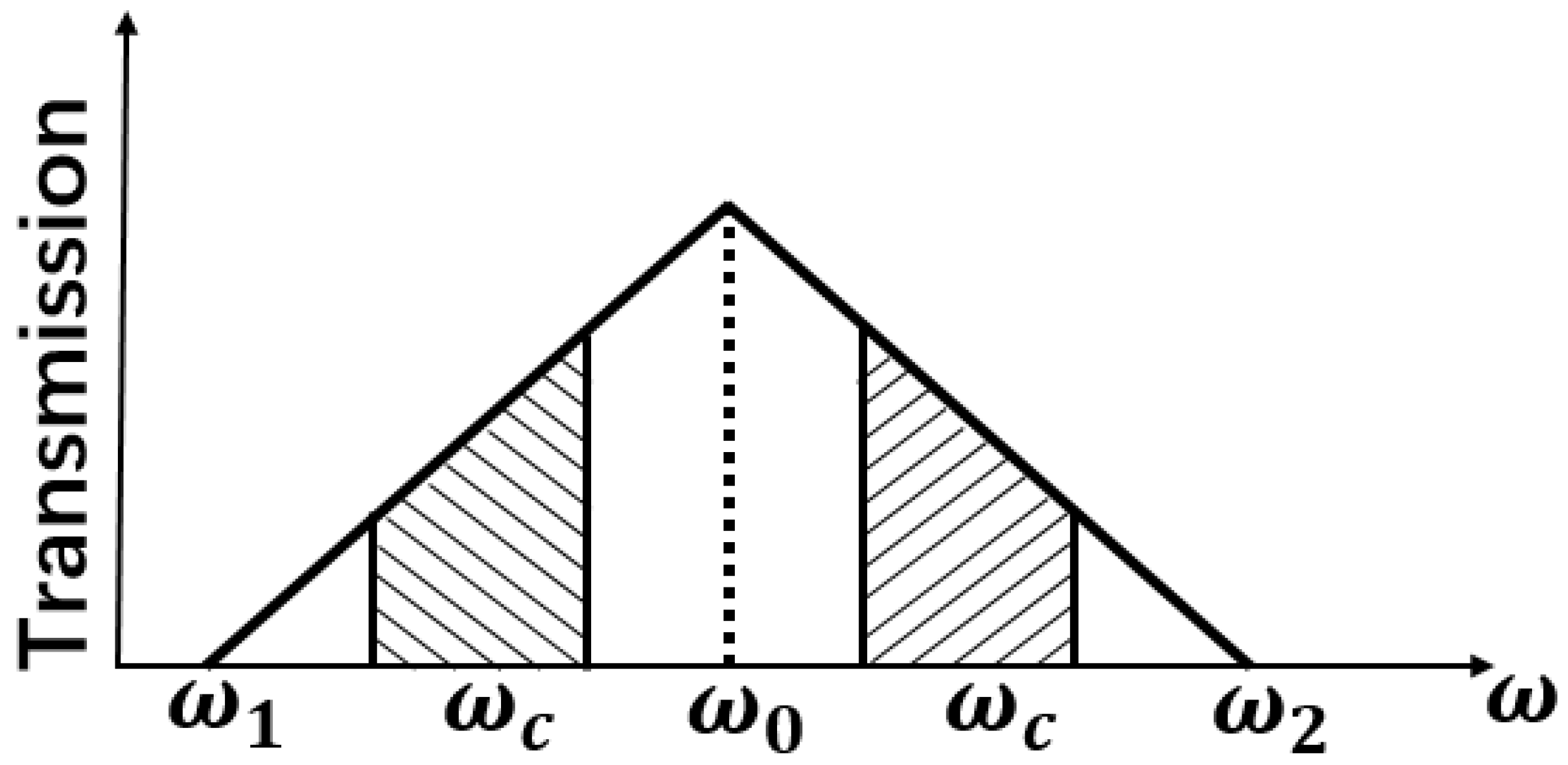
Equation (2) shows that the chirp $△v\left(t\right)$ is a linear function of the drive signal, but it has the opposite sign to $p\left(t\right)$. As we know, an optical filter with a linear filtering window can be regarded as a frequency discriminator, which can linearly map the chirp to intensity [16]. Its transmission curve is shown in Figure 1.

The corresponding spectral transfer function is written as

$$H\left(\omega \right)=\left\{\begin{array}{cc}K\left(\omega -{\omega }_1\right)\hfill & {\omega }_1<{\omega }_c<{\omega }_0\hfill \\ -K\left(\omega -{\omega }_2\right)\hfill & {\omega }_0<{\omega }_c<{\omega }_2\hfill \end{array}\right.,$$

(3)

where K and −K are the slope of the rising and falling edges of the filtering window, respectively. Here, the conditions of the central wavelength ${\omega }_c$ of the chirped signal located at the linear edge of the filtering window and its bandwidth completely covered by the linear part are assumed. After passing through such a filter, the output of the chirped signal can be deduced as [16]

$$p_{\mathrm{out}}\left(t\right)=\left\{\begin{array}{cc}[M-Np(t\left)\right]p\left(t\right)\hfill & {\omega }_1<{\omega }_c<{\omega }_0\hfill \\ [M+Np(t\left)\right]p\left(t\right)\hfill & {\omega }_0<{\omega }_c<{\omega }_2\hfill \end{array}\right.,$$

(4)

where $M=K^2({\omega }_c-{\omega }_1)$ or $M=K^2({\omega }_2-{\omega }_c)$, $N=\frac{\alpha \kappa }{2}{K}^2({\omega }_c-{\omega }_1)$ or $N=\frac{\alpha \kappa }{2}{K}^2({\omega }_2-{\omega }_c)$ are constants. Therefore, the signal after the frequency discriminator is the multiplication of two functions, which are the envelope function and the chirp function. The output expression $M-Np\left(t\right)$ or $M+Np\left(t\right)$ can be understood as a mapping of chirp to intensity. An interesting thing is that when the optical carrier is placed on the rising edge of the filter window, the chirp-to-intensity mapping gives the opposite phase, while it gives the same phase when placing the optical carrier on the falling edge of the filtering window. At the same time, placing the carrier at different heights of the filtering window edge results in different direct currents (DCs) on the mapped intensity signal. Obviously, Equation (4) implies that a parabolic pulse can be achieved once the input signal $p\left(t\right)$ is a triangular pulse.

As described by Equation (2), a modulated triangular pulse has an intensity profile of $p\left(t\right)$ and a chirp of $△v\left(t\right)=-\frac{\alpha \kappa }{4\pi }p\left(t\right)$ if the laser bias current is much larger than the threshold. Meanwhile, assuming that there is a filter with a sufficient filtering window width, placing the carrier at different positions will result in countless chirp-to-intensity mappings. As can be seen from Equation (4), there are two typical chirp-to-intensity mappings, $M-Np\left(t\right)$ and $M+Np\left(t\right)$, which are represented as $△v_{mapping-1}$ and $△v_{mapping-2}$, respectively. Specifically, placing the optical carrier at two different positions on the rising edge of the filtering window yields two special chirp-to-intensity mappings. Thus, three types of parabolic pulses can be generated.

In general, a normalized triangular pulse stream $p\left(t\right)$ in the first period can be written as [17]:

$$p\left(t\right)=\left\{\begin{array}{cc}\frac{2}{T}t\hfill & t\in [0,\frac{T}{2}]\hfill \\ -\frac{2}{T}t+2\hfill & t\in [\frac{T}{2},T]\hfill \end{array}\right.,$$

(5)

where T is the period of the triangular pulse.

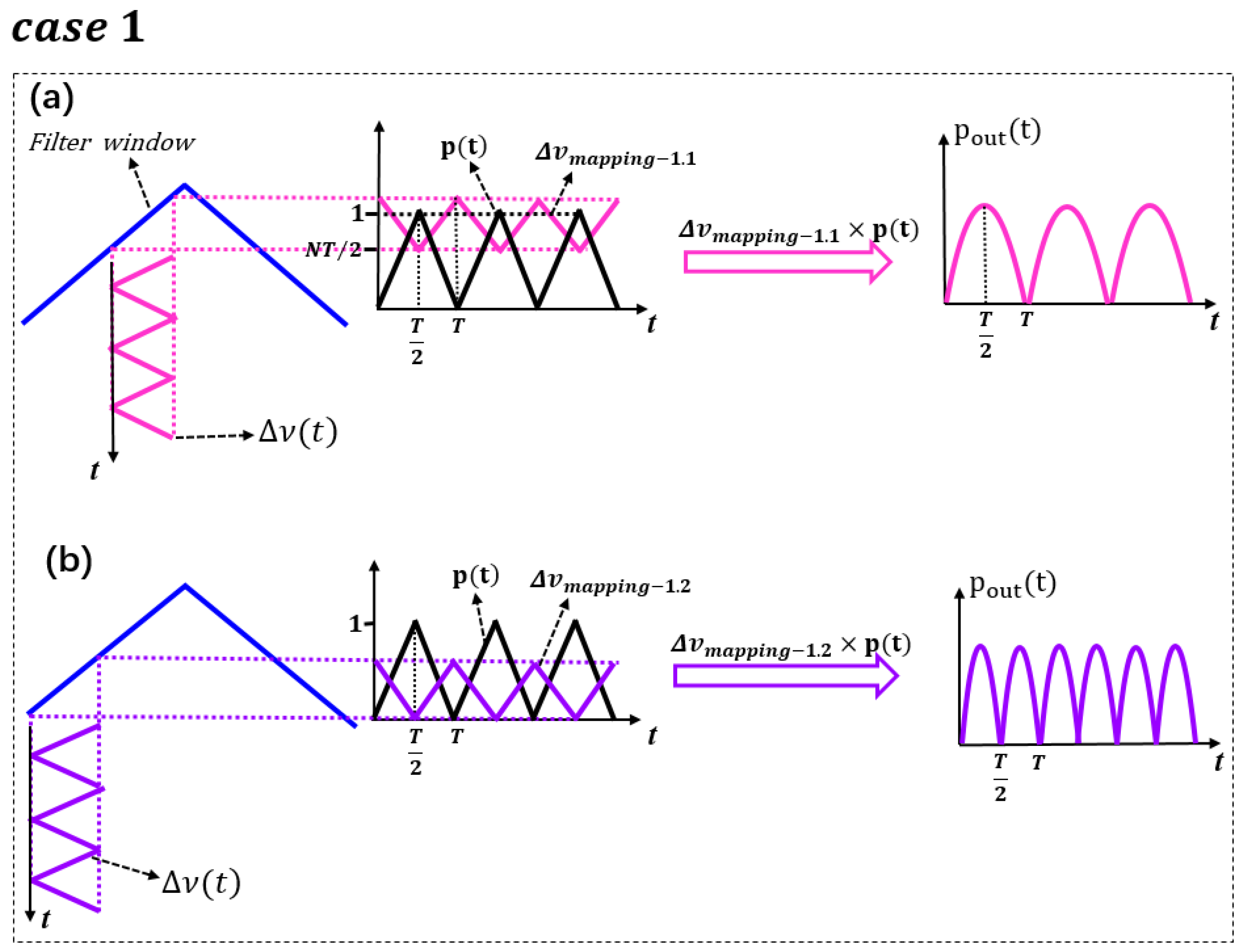
Case 1 is shown in Figure 2. The optical carrier is placed on the rising edge of the filtering window, where $△v_{mapping-1}$ and $p\left(t\right)$ are out of phase. At this point, by adjusting the position of the central wavelength in the filtering window, there are two special values, whose corresponding chirp-to-intensity mappings are represented as $△v_{mapping-1.1}$ and $△v_{mapping-1.2}$.

When the optical carrier is located at the upper part of the rising edge of the filtering window, one adjusts the window to change the value in Equation (4) so that the DC difference between the mapped intensity $△v_{mapping-1.1}$ and $p\left(t\right)$ is $NT/2$, as shown in Figure 2a.

Mathematically, $△v_{mapping-1.1}$ features the triangular profile, so it can be expressed as:

$$▵v_{mapping-1.1}\left(t\right)=\left\{\begin{array}{cc}-Nt+NT\hfill & t\in [0,\frac{T}{2}]\hfill \\ Nt\hfill & t\in [\frac{T}{2},T]\hfill \end{array}\right..$$

(6)

Since the signal originally has an envelope of $p\left(t\right)$, after the filter, the composite signal is the spontaneous multiplication of $△v_{mapping-1.1}$ and $p\left(t\right)$, which can be expressed as:

$$p\left(t\right)\times ▵v_{mapping-1.1}\left(t\right)=-\frac{2N}{T}{t}^2+2Ntt\in [0,T].$$

(7)

From Equation (7), the parabolic expressions for the first and second half periods are the same, and the coefficient of the quadratic term is negative. The curve changes from minimum to maximum in the interval $[0,T/2]$ and from maximum to minimum in the interval $[T/2,T]$, resulting in a bright parabola with a vertex at $T/2$. This indicates the generation of a bright parabolic pulse stream with the same period as the triangular drive signal. Another point is that the amplitude of the mapped intensity does not affect the shape of the multiplied parabolic pulse.

Then, by slightly shifting the filtering window, the optical carrier is located in the lower part of the rising edge of the filtering window. In this case, the mapped intensity $△v_{mapping-1.2}$ has the same DC as $p\left(t\right)$ and gives an intensity function of $p\left(t\right)$ with an inverse phase, as shown in Figure 2b. At this time, $△v_{mapping-1.2}$ and its multiplication by $p\left(t\right)$ can be expressed as:

$$▵v_{mapping-1.2}\left(t\right)=\left\{\begin{array}{cc}-Nt+\frac{NT}{2}\hfill & t\in [0,\frac{T}{2}]\hfill \\ Nt-\frac{NT}{2}\hfill & t\in [\frac{T}{2},T]\hfill \end{array}\right.,$$

(8)

$$p\left(t\right)\times ▵v_{mapping-1.2}\left(t\right)=\left\{\begin{array}{cc}-\frac{2N}{T}{t}^2+Nt\hfill & t\in [0,\frac{T}{2}]\hfill \\ -\frac{2N}{T}{t}^2+3Nt-NT\hfill & t\in [\frac{T}{2},T]\hfill \end{array}\right..$$

(9)

It can be seen from Equation (9) that the coefficient of the quadratic term is negative. One interesting thing is that there are two parabolic pulses within the time interval of T, which indicates that the generated parabolic pulse stream has a repetition frequency twice that of the triangular drive signal.

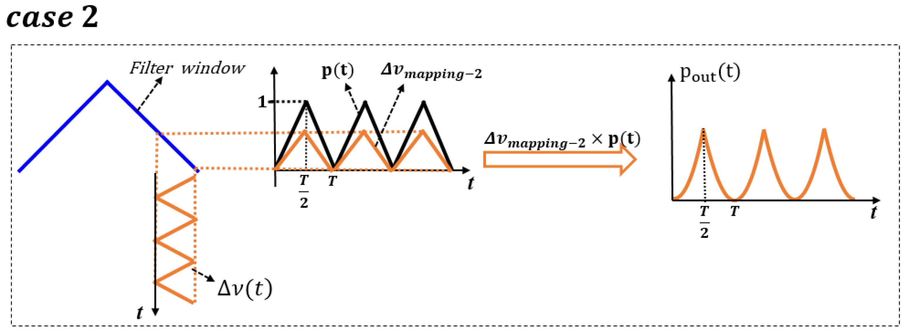
Similarly, when the optical carrier is placed on the falling edge of the filtering window, case 2 is achieved, as shown in Figure 3. The mapped intensity $△v_{mapping-1.2}$ and $p\left(t\right)$ are out of phase; furthermore, the DC between them is the same.

In this case, $△v_{mapping-1.2}$ and its multiplication by $p\left(t\right)$ can be expressed as:

$$▵v_{mapping-2}\left(t\right)=\left\{\begin{array}{cc}Nt\hfill & t\in [0,\frac{T}{2}]\hfill \\ -Nt+NT\hfill & t\in [\frac{T}{2},T]\hfill \end{array}\right.,$$

(10)

$$p\left(t\right)\times ▵v_{mapping-2}\left(t\right)=\left\{\begin{array}{cc}\frac{2N}{T}{t}^2\hfill & t\in [0,\frac{T}{2}]\hfill \\ \frac{2N}{T}{t}^2-4Nt+2NT\hfill & t\in [\frac{T}{2},T]\hfill \end{array}\right..$$

(11)

From Equation (11), it can be seen that the coefficient of the quadratic term parabolas is positive, which gives a dark parabolic pulse. The function value in the interval $[0,T/2]$ increases from a minimum to a maximum, and decreases from the same maximum to the same minimum in the interval $[T/2,T]$. Thus, Equation (11) presents a periodic dark parabolic stream with the same period of the triangular drive signal.

As one can see from Equations (7), (9) and (11), all three situations are parabolas with different characteristics. The first case generates bright parabolic pulses of fundamental and double frequencies, while the second case generates a dark parabolic pulse. In particular, by comparing Figure 2a,b, the multiplication results present obvious differences with different DCs because a small fluctuation in the parameters for the multiplication operation can have a significant impact on the results.

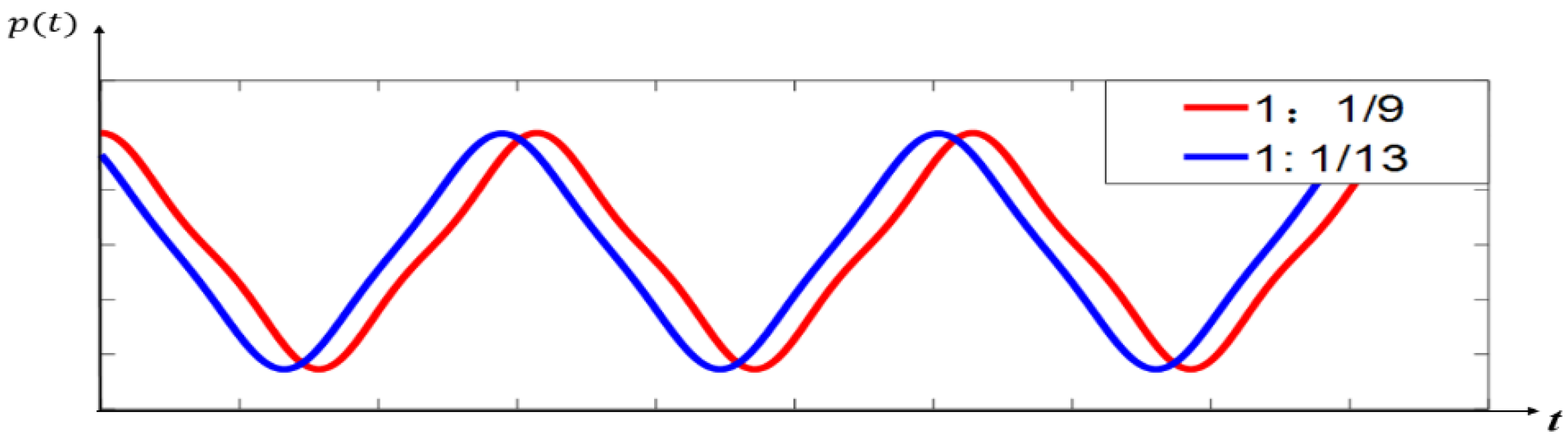
Mathematically, the Fourier expansion of a periodic triangular signal is [18]

$$T_{tr}\left(t\right)=C_{tr}+D_{tr}\sum _{k=1,3,5}^{\infty }\frac{1}{k^2}cos(k\Omega t),$$

(12)

where $C_{tr}$ and $D_{tr}$ are two constants and $\Omega$ is the fundamental angular frequency. Usually, a triangular waveform with second-order approximation is good enough. However, in order to obtain a triangular pulse with a better linear edge, one can adjust the coefficient ratio of harmonic components appropriately within a certain tolerance range, and the optimized triangular waveform can be expressed as

$$T_{tr}\left(t\right)=DC+cos(\Omega t)+\left(\frac{1}{13}\right)cos(3\Omega t).$$

(13)

By comparing the coefficient ratio of harmonic components (1:1/9 and 1:1/13), as seen in Figure 4, the linear edge of the optimized triangular waveform is greatly improved.

To further evaluate the quality of the optimized and standard waveform, we introduce the goodness of fit in mathematical statistics to evaluate the results, which is defined as the fitting degree between the regression line and the observed value and expressed as

$$\begin{array}{c}\hfill R^2=1-\frac{{\sum }_{i=1}^n{(y_i-{\widehat{y}}_i)}^2}{{\sum }_{i=1}^n{(y_i-\overline{y})}^2},\end{array}$$

(14)

where $y_i$ is the calculated value, ${\widehat{y}}_i$ is the average value of the calculated value and $\overline{y}$ is the standard value. If $R^2$ is closer to 1, the fitting effect will be better [19,20]. The optimized triangular waveform is 0.9696. Starting from the triangular pulse, the $R^2$ values of the generated three parabolic waveforms are 0.9967, 0.9967 and 0.9754, respectively, which shows that the obtained parabolic pulses are acceptable.

3. Experiments and Results

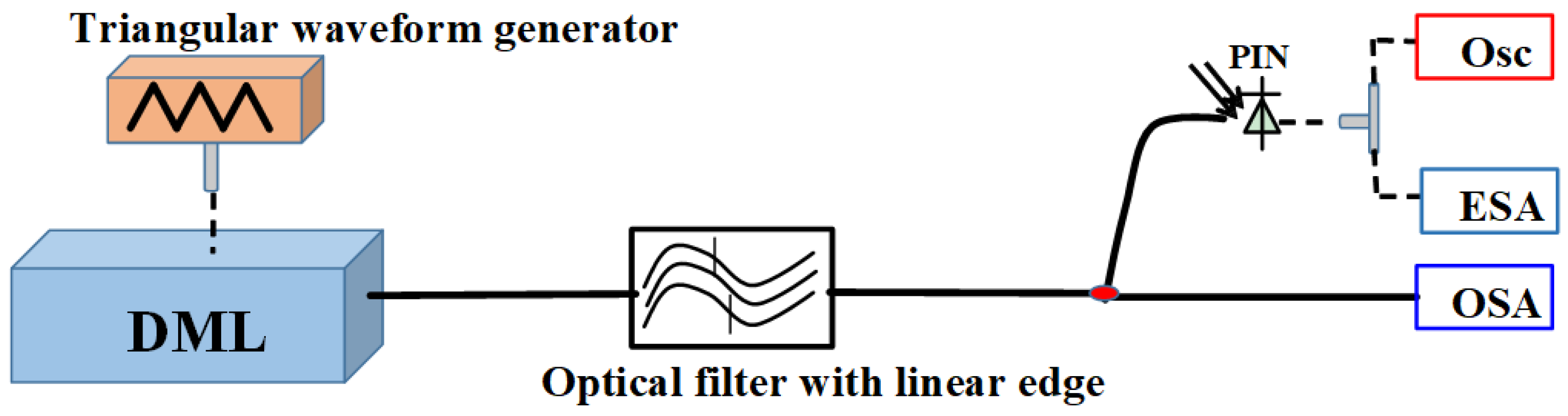
To verify the feasibility of the proposed parabolic waveform generator, an experimental demonstration with the configuration shown in Figure 5 was implemented. The system mainly includes a triangular pulse generator, a DML and an optical filter. In this system, the distributed feedback DML (DFB-DML) is the key device, and it has a modulation bandwidth of 18 GHz, a threshold current of 30 mA, an output power of 11 dBm and a cavity length of about 200 um. To satisfy the operation requirements mentioned before, the bias current was set at 80 mA. The frequency bandwidth of the used photodetector (PD, Finisar XPDV210R) is 50 GHz.

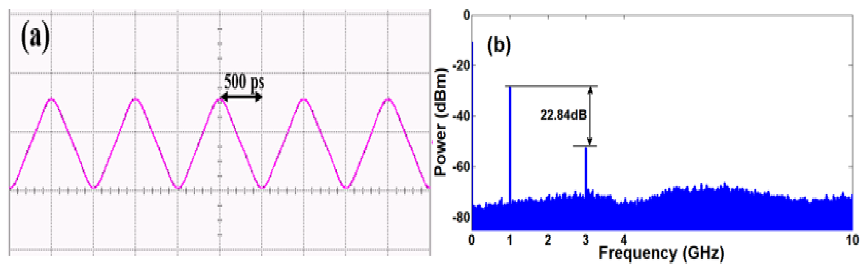
Firstly, a triangular waveform generator outputs a 1 GHz drive signal with second-order approximation. The corresponding waveform and electrical spectrum are monitored by an oscilloscope (86100D Infiniium DCA−X, Agilent, Santa Clara, CA, USA) and an electrical spectrum analyzer (ESA, Agilent N9010A EXA), respectively, as shown in Figure 6a,b. From the electrical spectrum, the power ratio between the first-order component and third-order component is 22.84 dB, which agrees with the expected coefficient ratio of 1:1/13.

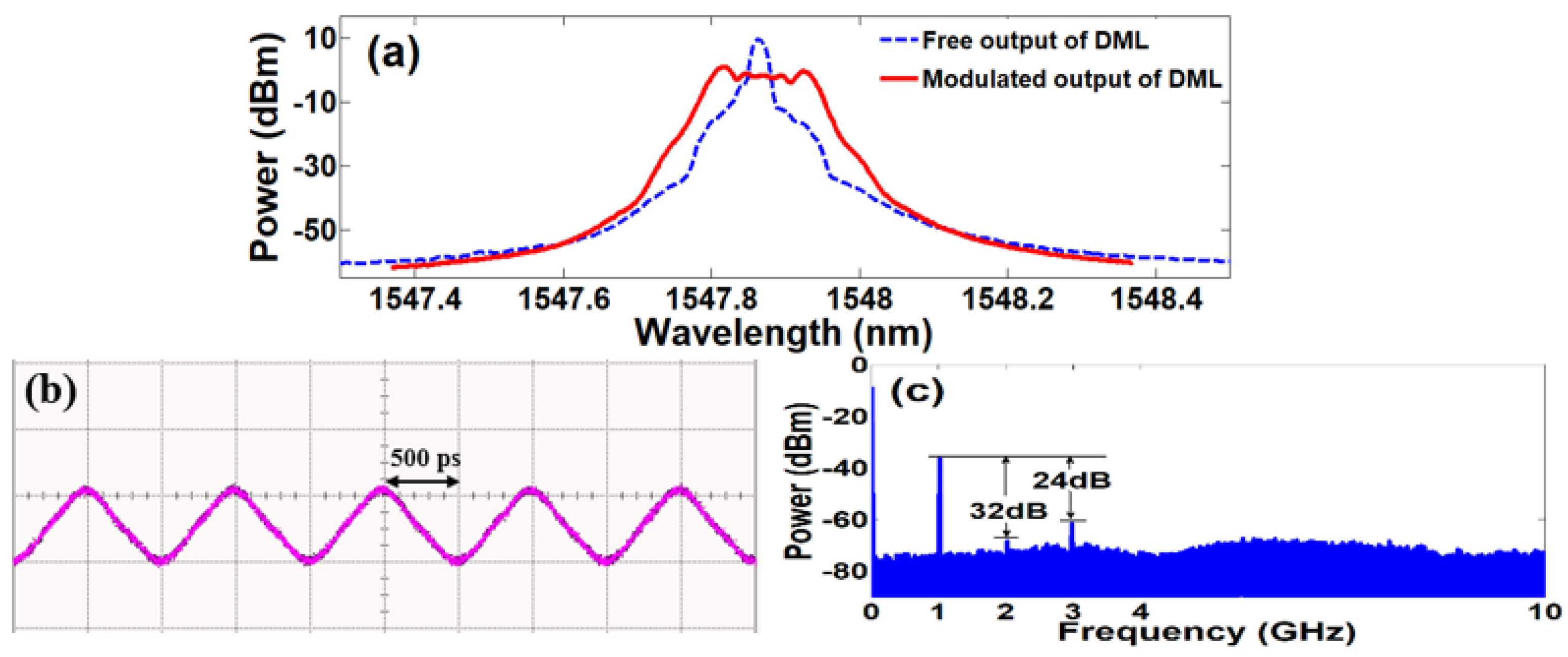
When the signal is applied on a DML with a wavelength of 1547.86 nm, optical triangular pulses with a certain chirp are generated, the optical spectrum of which was measured via an optical spectrum analyzer (OSA, YOKOGAWA AQ6370C), as shown in Figure 7a. Waveform and electrical spectra are given in Figure 7b,c. Clearly, the modulated signal is a triangular pulse, which is the same as the input signal. A Gaussian optical filter (Optical Tunable Filter, OTF−320) can linearly map the chirp signal to the intensity signal in the time domain because it has a quasi-linear edge. 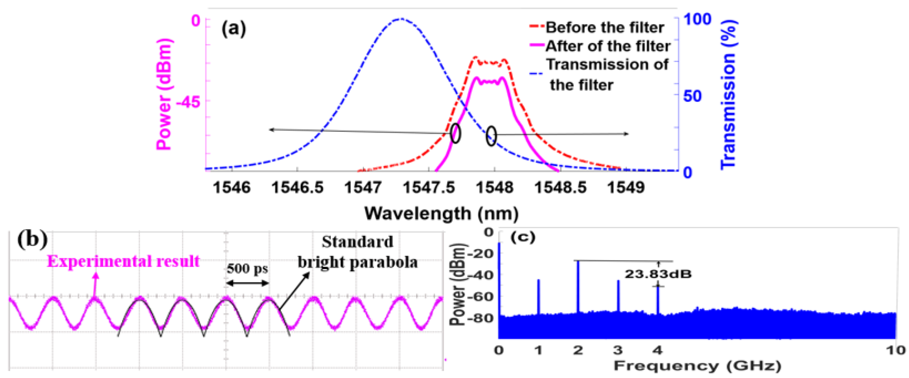For the three different cases described in Section 2, experiments were carried out one by one. In case 1, by setting the carrier on the upper part of the rising edge of the filter, a bright parabolic waveform can be output, as given by Figure 8b.

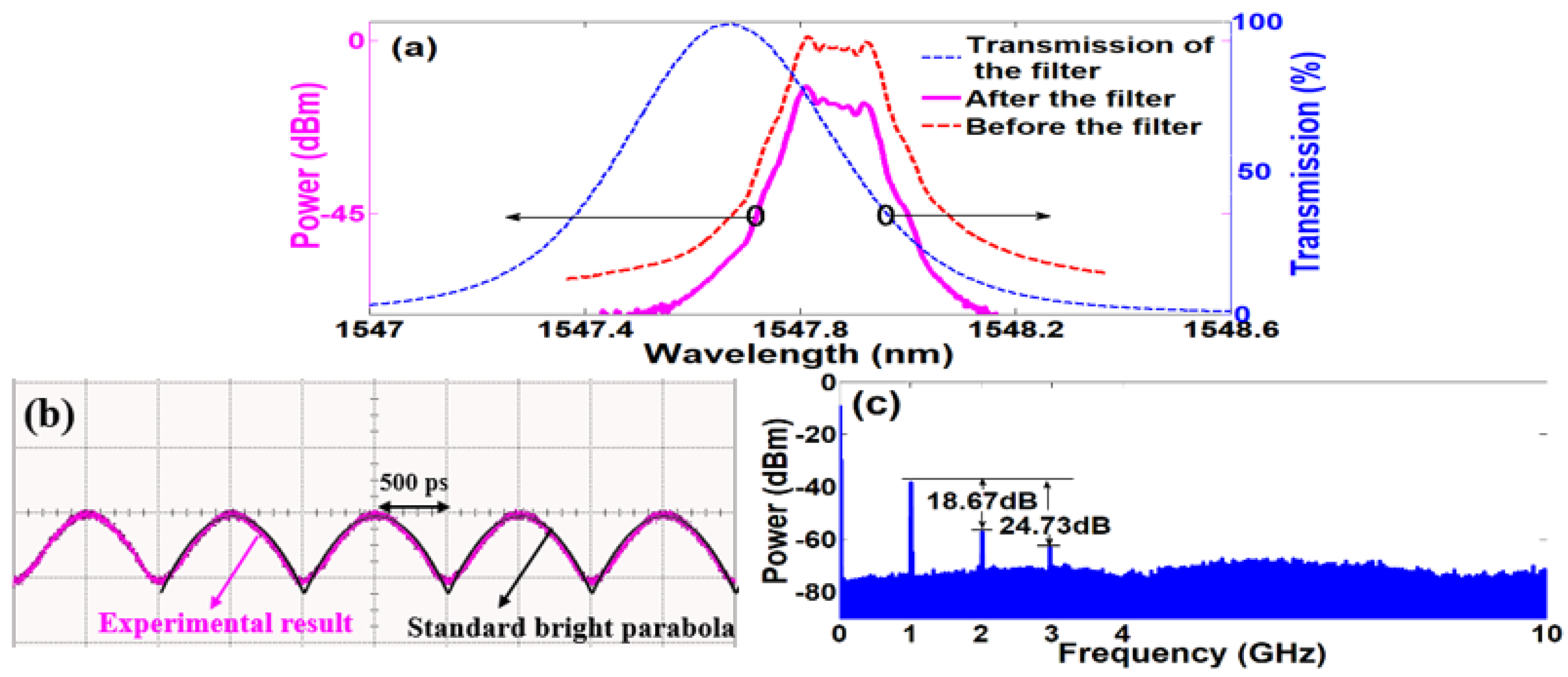
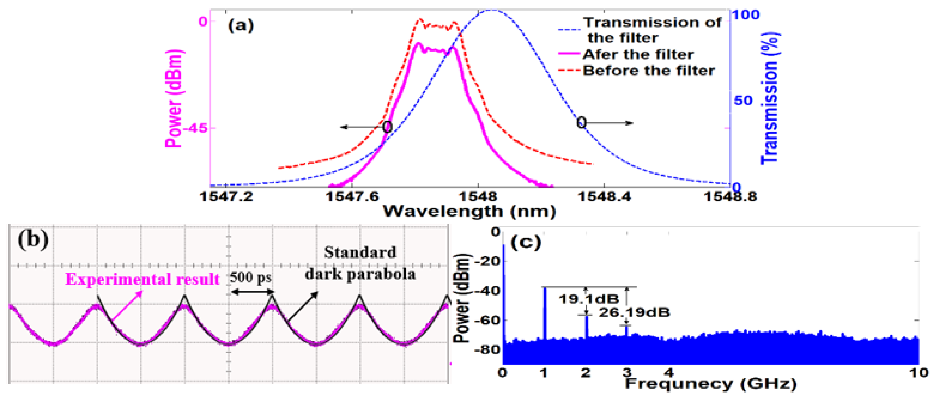
At the same time, the carrier was placed at the lower part of the rising edge of the filter, which leads to a bright parabolic pulse with a doubled frequency, as shown in Figure 9. Finally, for case 2, by fine tuning the filter window, the optical carrier is located at the falling edge of the filter, as shown in Figure 10a. It should be noted that we mainly adjust the window of the filter to obtain the desired filtering position during the operation, because the wavelength of the DML is fixed. This process transforms the triangular pulse to a dark parabolic pulse. Figure 10b,c gives the corresponding waveform and electrical spectra. The experimental result is consistent with the standard parabolic waveform.

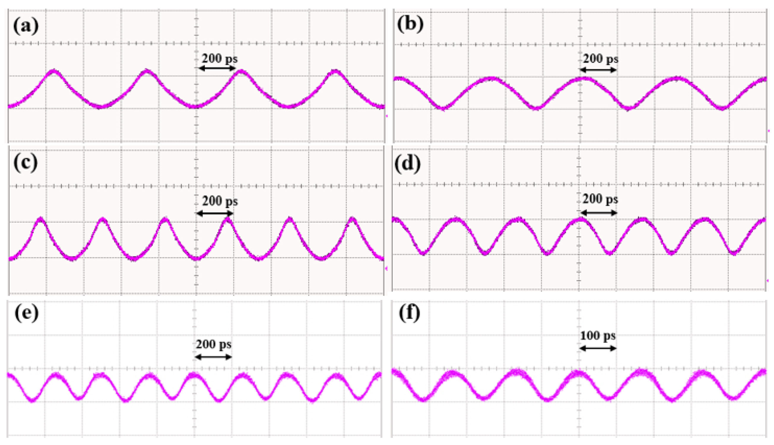
Figure 11 shows the tunability of the system. Dark, bright and the doubled bright parabolic waveforms with repetition frequencies of 2 and 3 GHz are generated under 2 GHz and 3 GHz triangular drive signals, respectively. From the experimental results shown above, this scheme presents good flexibility and results in all cases.

4. Discussion

From the calculation results, the degree of fitting values of the parabolic pulses with a fundamental frequency or a doubled frequency is almost the same. However, in the experimental results, the quality of the parabolic pulses with doubling frequency seems worse than that of the fundamental frequency. This is because the falling edge of a Gaussian filter has better linearity in the upper region than in the lower region, so the quality of the triangular waveform mapped by the former case is better. In theory, if an optical filter with a wider range of linear edges is employed, the quality of the parabolic pulses with a doubled frequency will be improved.

An optical filter with an ideal linear edge to linearly map the chirp signal is usually not easy to obtain, but Gaussian filters, delay interferometers and specially designed FBGs can be employed, because these filters have filtering windows with quasi-linear edges. These replacements are also able to function well and have been experimentally verified in [21,22,23].

Based on the principle analysis and experimental results, compared with existing schemes, our system makes full use of the chirp characteristics of DMLs, and the chirp signal can be easily mapped from the frequency domain to the time domain by an optical filter with linear edges. By simply adjusting the filtering window, the modulated optical envelope and mapped chirp signal are able to synthesize parabolic waveforms of multiple types and a good quality. This method only requires common commercial devices, and the operation process is simple and stable; thus, it is a new approach for parabolic pulse generation with good application prospects.

5. Conclusions

In summary, a simpler parabolic waveform generator scheme based on frequency–time mapping is proposed and experimentally verified. The chirp characteristics of the semiconductor laser are fully explored and utilized. Theoretically, the generation conditions for implementing parabolic pulse generation have been analyzed. In the experiments, by simply adjusting the filter window of the optical filter, dark parabola, bright parabola with a fundamental frequency and bright parabola with a doubled frequency were successfully obtained, and agree well with the standard waveform. The significance of the proposed scheme is that useful waveforms can be generated by arranging the modulation envelope and the corresponding chirp from a directly modulated laser, since a directly modulated LD is the most popular device and the chirp can be easily mapped to an intensity signal via an optical filter. Therefore, the proposed scheme may provide a simple and low-cost waveform generator to generate some special waveforms.

References

1. Godil, A.A.; Auld, B.A.; Bloom, D.M. Time lens producing 1.9 ps optical pulses. Appl. Phys. Lett. 1993, 62, 1047–1049. [Google Scholar] [CrossRef]
2. Bennett, C.V.; Kolner, B.H. Up conversion time microscope demonstrating 103 magnification of femtosecond waveforms. Opt. Lett. 1999, 24, 783–785. [Google Scholar] [CrossRef] [PubMed]
3. Howe, J.V.; Hansryd, J.; Xu, C. Multiwavelength pulse generator using time-lens compression. Opt. Lett. 2004, 29, 1470–1472. [Google Scholar] [CrossRef] [PubMed]
4. Foster, M.A.; Salem, R.; Okawachi, Y.; Turner-Foster, A.C.; Lipson, M.; Gaeta, A.L. Ultrafast waveform compression using a time-domain telescope. Nat. Photonics 2009, 3, 581–585. [Google Scholar] [CrossRef]
5. Wu, R.; Supradeepa, V.R.; Long, C.M.; Leaird, D.E.; Weiner, A.M. Generation of very flat optical frequency combs from continuous-wave lasers using cascaded intensity and phase modulators driven by tailored radio frequency waveforms. Opt. Lett. 2010, 35, 3234–3236. [Google Scholar] [CrossRef] [PubMed]
6. Kolner, B.H. Space-time duality and the theory of temporal imaging. IEEE J. Quantum. Electron. 1994, 30, 1951–1963. [Google Scholar] [CrossRef]
7. Latkin, A.I.; Turitsyn, S.K.; Sysoliatin, A.A. Theory of parabolic pulse generation in tapered fiber. Opt. Express 2007, 32, 331–333. [Google Scholar] [CrossRef]
8. Hirookaand, T.; Nakazawa, M. Parabolic pulse generation by use of a dispersion-decreasing fiber with normal group-velocity dispersion. Opt. Lett. 2003, 29, 498–500. [Google Scholar] [CrossRef]
9. Hirooka, T.; Nakazawa, M.; Okamoto, K. Bright and dark 40 GHz parabolic pulse generation using a picosecond optical pulse train and an arrayed waveguide grating. Opt. Lett. 2008, 33, 1102–1104. [Google Scholar] [CrossRef]
10. Nguyen, D.; Piracha, M.U.; Mandridis, D.; Delfyett, P.J. Dynamic parabolic pulse generation using temporal shaping of wavelength to time mapped pulses. Opt. Express 2011, 19, 12305–12311. [Google Scholar] [CrossRef]
11. Wei, C.; Jiang, Y.; Wang, R.; Liu, H.; Yu, Q.; Chen, X.; Tian, J. Tunable parabolic pulses generation by mapping transmissivity curve of Mach–Zehnder modulator to time domain. Opt. Eng. 2021, 60, 036105. [Google Scholar] [CrossRef]
12. Wang, R.; Jiang, Y.; Wei, C.; Liu, H. Parabolic pulse generation based on a multiply operation of two triangular pulses. Opt. Eng. 2020, 59, 100502. [Google Scholar] [CrossRef]
13. Wang, R.; Jiang, Y.; Wei, C.; Chen, X.; Yu, Q. Parabolic pulses generation based on nonlinear optical fiber loop mirror. Opt. Eng. 2021, 60, 096102. [Google Scholar] [CrossRef]
14. Tucke, R.S. High-speed modulation of semiconductor lasers. IEEE Trans. Electron. Devices 1985, 2, 2572–2584. [Google Scholar] [CrossRef]
15. Yousuf, A.; Najeeb-ud-din, H. Effect of gain compression above and below threshold on the chirp characteristics of 1.55 um distributed feedback laser. Opt. Rev. 2016, 23, 897–906. [Google Scholar] [CrossRef]
16. Chen, X.P.; Jiang, Y.; Yu, Q.; Xu, J.; Zi, Y.; Li, J.; Chen, N. All-optical microwave waveform transformation based on photonic temporal processors. Opt. Express 2022, 30, 10428–10442. [Google Scholar] [CrossRef]
17. Jiang, Y.; Ma, C.; Bai, G.; Qi, X.; Tang, Y.; Jia, Z.; Wu, T. Photonic microwave waveforms generation based on time-domain processing. Opt. Express 2015, 23, 19442–19452. [Google Scholar] [CrossRef]
18. Ma, C.; Jiang, Y.; Bai, G.; Tang, Y.; Qi, X.; Jia, Z.; Yu, J. Photonic generation of microwave triangular waveform based on polarization-dependent modulation efficiency of a single-drive Mach–Zehnder modulator. Opt. Commun. 2016, 23, 207–210. [Google Scholar] [CrossRef]
19. Tjur, T. Coefficients of determination in logistic regression models—A new proposal: The coefficient of discrimination. Am. Stat. 2009, 63, 366–372. [Google Scholar] [CrossRef]
20. Kasuya, E. On the use of R and R squared in correlation and regression. Ecol. Res. 2019, 34, 235–236. [Google Scholar] [CrossRef]
21. Zhang, L.; Wu, J.; Yin, X.; Sun, X.; Cao, P.; Jiang, X.; Su, Y. A High-Speed Second-Order Photonic Differentiator Based on Two-Stage Silicon Self-Coupled Optical Waveguide. IEEE Photonics J. 2014, 6, 7900505. [Google Scholar] [CrossRef]
22. Dong, J.; Luo, B.; Zhang, Y.; Huang, D.; Zhang, X. Reconfigurable photonic differentiators based on all-optical phase modulation and linear filtering. Opt. Commun. 2011, 284, 5792–5797. [Google Scholar] [CrossRef]
23. Velanas, P.; Bogris, A.; Argyris, A.; Syvridis, D. High-speed all-optical first-and second-order differentiators based on cross-phase modulation in fibers. J. Lightwave Technol. 2008, 26, 3269–3276. [Google Scholar] [CrossRef]
Figure 1. Transmission curve of the optical filter with a linear edge.
Photonics 11 00004 g001
Figure 2. Graphical representation of bright parabolic pulse generation. (a) The generation of a bright parabola with a fundamental frequency. (b) The generation of a frequency-doubled bright parabola.
Photonics 11 00004 g002
Figure 3. Graphical representation of dark parabolic pulse generation.
Photonics 11 00004 g003
Figure 4. Triangular graphical representation with coefficient ratios of 1:1/9 and 1:1/13.
Photonics 11 00004 g004
Figure 5. The experimental configuration of the proposed parabolic waveform generator. DML: directly modulated laser; Osc: oscilloscope; ESA: electrical spectrum analyzer; OSA: optical spectrum analyzer.
Photonics 11 00004 g005
Figure 6. Measurement results of input triangular pulse. (a) The triangular waveform. (b) The corresponding electrical spectrum.
Photonics 11 00004 g006
Figure 7. Measured results of a DML modulated by a triangular signal. (a) The modulated optical spectrum with the repetition frequency of 1 GHz. (b) The output waveform. (c) The corresponding electrical spectrum.
Photonics 11 00004 g007
Figure 8. The filtering results of the carrier on the upper of the falling edge. (a) The output spectrum. (b) Generated bright parabolic pulse. (c) The corresponding electrical spectrum.
Photonics 11 00004 g008
Figure 9. The filtering results of the carrier on the lower of the rising edge. (a) The output spectrum. (b) Generated bright parabolic pulse with doubled frequency. (c) The corresponding electrical spectrum.
Photonics 11 00004 g009
Figure 10. The filtering results of the carrier on the falling edge. (a) The output spectrum. (b) Generated dark parabolic pulse. (c) The corresponding electrical spectrum.
Photonics 11 00004 g010
Figure 11. Experiment results: (a) 2 GHz dark parabolic waveform with 2 GHz drive signal; (b) 2 GHz bright parabola with 2 GHz drive signal; (c) 3 GHz dark parabola with 3 GHz drive signal; (d) 3 GHz bright parabola with 3 GHz drive signal; (e) 4 GHz bright parabolic pulse with 2 GHz drive signal; (f) 6 GHz bright parabolic pulse with 3 GHz drive signal.
Photonics 11 00004 g011
Disclaimer/Publisher’s Note: The statements, opinions and data contained in all publications are solely those of the individual author(s) and contributor(s) and not of MDPI and/or the editor(s). MDPI and/or the editor(s) disclaim responsibility for any injury to people or property resulting from any ideas, methods, instructions or products referred to in the content.