1. Introduction
Cavity optomechanics studying the interaction between light and mechanical oscillation has recently become a rapidly developing field and now plays an important role in many fields of physics, including cooling of mechanical oscillators [
1,
2,
3], gravitational-wave detectors [
4], manipulation of light propagation [
5,
6,
7], integrated optical components [
8], and so on [
9]. Numerous studies have shown that many interesting effects uncovered in atomic-molecular systems can also be observed in the optomechanical system through mechanical effects of light. A classical example is optomechanically induced transparency/absorption (OMIT), which has been predicted theoretically [
10,
11,
12] and verified experimentally [
13,
14,
15]. OMIT, a direct analog of electromagnetically induced transparency, is a kind of induced transparency caused by the radiation pressure of coupling light to mechanical oscillator modes, in which the transmission of a probe field can be regulated all-optically by using a strong driving field, and can be well described through the linearization of optomechanical interactions. More specifically, the optomechanical system is pumped by a strong driving field with frequency
and a weak detection field with frequency
. Then, a spectrum of frequency
appears in the output field, where
n is an integer representing the
n-order sideband [
16,
17,
18,
19,
20]. For example, the output fields with frequencies
and
denote the first- and second-order upper or lower sideband [
16], respectively. In particular, based on the linearized dynamics of the optomechanical interactions
, a transparent window for the propagation of the probe field is induced by the incident field when the resonance condition is satisfied. It has been shown that this intriguing phenomenon provides a unique platform for achieving precision measurement [
21,
22,
23,
24,
25,
26,
27,
28,
29], such as precision measurement of electrical charges with OMIT [
23] and mass sensor with an optomechanical microresonator [
24].
Nonlinear cavity optomechanics has recently been the topic of widespread investigations and has developed enormously over the past decades. Many interesting phenomena deriving from the nonlinear optomechanical interactions have been uncovered [
30,
31,
32,
33,
34,
35,
36,
37], ranging from higher-order sidebands generation [
19,
20,
26] and cavity optomechanical chaos [
33,
36] to the Kuznetsov–Ma soliton in a microfabricated optomechanical array [
32]. An analytical method of describing the nonlinear optomechanical interaction has been proposed. One of the most typical examples is the second-order sideband generation [
16] when the nonlinear term of the system was taken into account. Furthermore, the traditional optomechanical system is further extended to the field of spintronics. Specifically, the generalized optomechanical system, which has a similar form of radiation-pressure-type interaction, and the interesting physical phenomenon of the sideband comb as well as the analogous laser action of magnons have been observed in the field of magnonics [
38,
39,
40]. Moreover, a large number of studies have shown that nonlinear interaction between cavity fields and mechanical oscillation in the optomechanical system may provide metrology with a higher precision and require less power [
28]; for example, the precision measurement of electrical charges beyond linearized dynamics [
25,
27], which can achieve the accuracy of measuring a single charge.
With the requirement of ultra-weak power and more accurate measurement, it is necessary to study the high-order nonlinear effects in the cavity optomechanical system. In this work, the third-order optomechanical nonlinearity based on the mechanical effect of light has been theoretically analyzed, which goes beyond the conventional linearized description of optomechanical interactions. Furthermore, the generation of a third-order sideband is analyzed in detail; that is, the sideband generation process with frequency component
from the output field, while
is the third-order upper sideband and
is the lower sideband. Physically, the generation of the high-order sideband is essentially the production and absorption process of multiple phonons caused by the nonlinear term of optomechanical interaction, which is consistent with the physical process of higher harmonic generation caused by the nonlinear term of interaction between light and atoms in atomic–molecular systems (i.e., the production and absorption process of multiple photons) [
41]. Therefore, the study of the high-order sideband is of great significance for understanding the nonlinear characteristics of optomechanical interaction and its related applications. Here, we only focus on third-order upper sideband generation and give its analytic expression by way of the perturbation method. We find that the amplitude of the third-order sideband can be substantively modified by OMIT where the spectrum of the third-order sideband is exactly the opposite of the OMIT spectrum. In addition, the relationship between the amplitude of the third-order sideband and the control field detuning
under the different driven frequency
was discussed in detail. We believe that the research of the third-order sideband generation will provide good theoretical guidance for the fundamental investigation of nonlinear cavity optomechanics [
42] and offer a nonlinear optical method with more accurate precision measurements.
The rest of this paper is organized as follows. In
Section 2, we introduce the physical patter of a traditional cavity optomechanical system and give the derivation of the Heisenberg–Langevin equation of motion in the presence of a strong pumping field and a weak probe field. Moreover, the third-order sideband generation induced by the higher-order optomechanical nonlinearity is discussed and the analytical expression is given. In
Section 3, the variation of the third-order sideband generation efficiency with the power of the control field is discussed in detail. Furthermore, we show that control field detuning plays an important role in the generation of the third-order sideband. Finally, a conclusion is presented in
Section 4.
2. Model and Dynamics
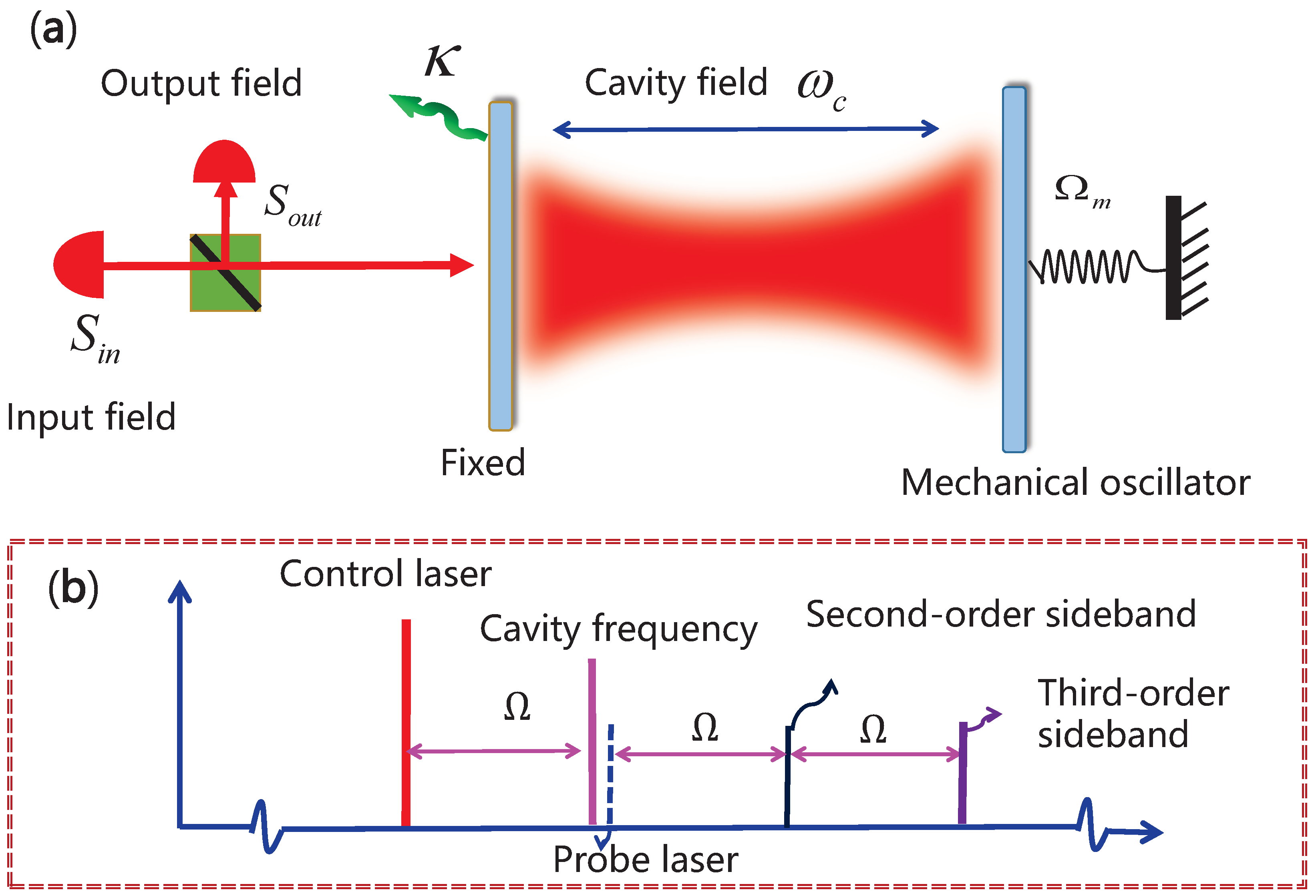
The physical pattern we consider is a traditional cavity optomechanical system, as diagrammatically shown in
Figure 1. The system consists of a hight-Q Fabry-Pérot cavity, in which one mirror is fixed and the other is movable and treated as a mechanical oscillator with effective mass
m and vibration frequency
. The single-mode cavity field with eigenfrequency
couples to the mechanical oscillator via optical radiation pressure. The Hamiltonian of this cavity optomechanical system, without loss of generality, reads as follows [
9]:
where the first two terms give the free Hamiltonian of the mechanical oscillator with
and
being the position and momentum operators of the movable mirror, respectively. The third term denotes the Hamiltonian of the cavity, in which the operators
and
are the bosonic annihilation and creation operators, which obey the commutation relations
,
. The last term describes the Hamiltonian interaction between the cavity field and the movable mirror with coupling strength G. Here, we presume that the optomechanical system is driven by a strong pumping field with frequency
and a weak probe field with frequency
. Therefore, the Hamiltonian of the driven optomechanical system can be written as follows:
Here,
represents the coupling parameter between the external input field and the cavity field, whose coupling value is selected as 1/2, and are used throughout the whole work.
are the amplitudes of the input field with
representing the pump power of the control field,
the power of the probe field and
the total decay rate of the cavity. In the rotating reference frame with frequency
of the input laser based on a unitary transformation
, the system Hamiltonian in Equation (
2) becomes
where
is the detuning between the cavity field frequency and the driving field frequency, and
is the beat frequency between the driving field and the probe field. After introducing the dissipation and fluctuation terms with the Markov approximation [
13], the dynamic evolution of the cavity optomechanical system governed by the Hamiltonian in Equation (
3) can be described by the following Heisenberg–Langevin equations:
where
with
,
,
,
and
Here,
indicates the dissipation rating of the mechanical oscillator, which is introduced phenomenologically. The noise matrix
with operators
and
denote environmental noises corresponding to the operators
and
. Here, we can assume that the quantum noise
has zero mean values, based on the nonvanishing commutation relations
and
. Furthermore, the thermal Langevin force
also has a vanishing mean value
, resulting from the temperature-dependent correlation function
[
43], where
and T are the Boltzmann constant and the temperature of the reservoir of the mechanical oscillator, respectively.
Equation (
4) can be solved by using the perturbation method. By using
and
where
with
, are the static solutions of the cavity field and the mechanical oscillator displacement for the case where the driving field is much stronger than the probe field and where all time derivatives vanish. Correspondingly,
and
are the fluctuations around the steady-state solutions of the cavity field
a and the mechanical displacement
x, respectively. After a simple calculus, we can obtain the nonlinear matrix equation that
and
satisfy, as shown above (under the mean-field approximation)
where
,
,
, and
Making the following ansatz [
44],
Substituting such ansatz into Equation (
6), we can get three sets of nonlinear matrix equations regarding the amplitude of the sidebands:
where
and
describe the first-, second-, and third-order sideband, respectively. Here, we should note that
when
, in other cases,
. The coefficient matrix
with
and
. The matrix
directly determines the magnitude of the effective sidebands amplitude and we call it the sideband matrix element.
describe the effect of OMIT and the second-order sideband, respectively, which have been obtained in previous work [
16], and
describes the effect of the third-order sideband of such an optomechanical system, which has not yet been studied.
Equations (
8) can easily be solved and
and
are obtained as follows:
and
where
and
and
From Equation (9), we can clearly get the mechanism of the sidebands generation: the first-order sideband is proportional to the amplitude of the probe field and the second-order sideband is mainly generated from the first-order sideband, and the third-order sideband is induced both by the first- and second-order sidebands. As a result, the effective sideband strength will be weaker and weaker, so it is particularly important to improve the intensity of the higher-order sideband generation.
The output field from the cavity optomechanical system can be acquired by using the standard input–output relationship [
45]:
The terms and describe the first-order upper sideband and lower sideband, respectively. The terms and express the second-order upper sideband and lower sideband, respectively. Without losing generality, the third-order upper sideband and lower sideband correspond to the term and , respectively.
The transmission of the probe field can be defined as the ratio between the amplitude of the output field and the probe field, as follows
By the same token, we can define a dimensionless expression
as the efficiency of the third-order sideband generation.
3. Results and Discussion
In the following section, we turn to discuss how the efficiency of the third-order upper sideband varies with the optical power of the control field
. After such discussion, we find that the efficiency of the third-order sideband process can be substantively modified by the control field. And more importantly, the amplitude of the third-order sideband can be enhanced by tuning the driven field detuning
. The simulation parameters used in this work are the effective mass of the mechanical oscillator
ng, the vibration frequency of the mechanical oscillator
MHz, the decay rate of the mechanical oscillator
kHz, the optomechanical coupling strength
GHz/nm, the detuning of the cavity field
, the total loss rate of the cavity field
MHz, and the drive field with wavelength
nm. These parameters are chosen from the experiment parameters [
13], and are used throughout the whole work.
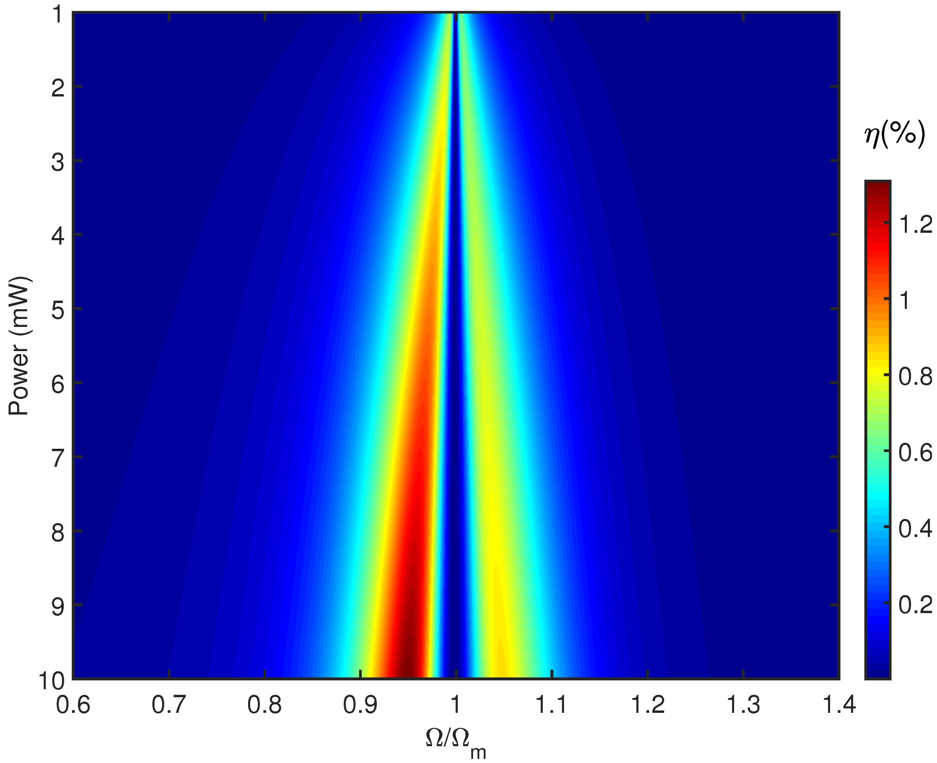
The efficiency of the third-order sideband process
varies with the driving frequency
and the power of control field
is plotted in
Figure 2. Here, we should note that the efficiency of the third-order sideband was used as
. As shown in
Figure 2, the depth of the color represents the efficiency of third-order sideband process
. The efficiency of the third-order sideband almost tends to zero near the resonance condition
(middle blue area). There is a transparent window under the resonance condition
and the probe light is completely transmitted, which leads to no excess light with which to induce the third-order sideband generation, so the efficiency of
is extremely weak. On both sides of
, however, the efficiency of the third-order sideband is enhanced, which means that there are two absorption valleys in the transmission spectrum. Under the circumstances, the probe field is almost completely absorbed and induces the generation of the third-order sideband. From above analysis, we can know that the spectral distribution of the third-order sideband is completely opposite to the first-order sideband.
Hence, we call it the optomechanically induced opacity of the third-order sideband, which means that the third-order sideband and even the higher-order sidebands are derived from the first-order sideband. From
Figure 2, we can see that the efficiency of third-order sideband generation increases as the optical power of the control field increases and the maximum value of
is about
, corresponding to the control field 10 mW. In addition, the width of the opacity window increases as the optical power of the control field increases, which coincides with the regular pattern of the first-order sideband varying with the power of the driven field.
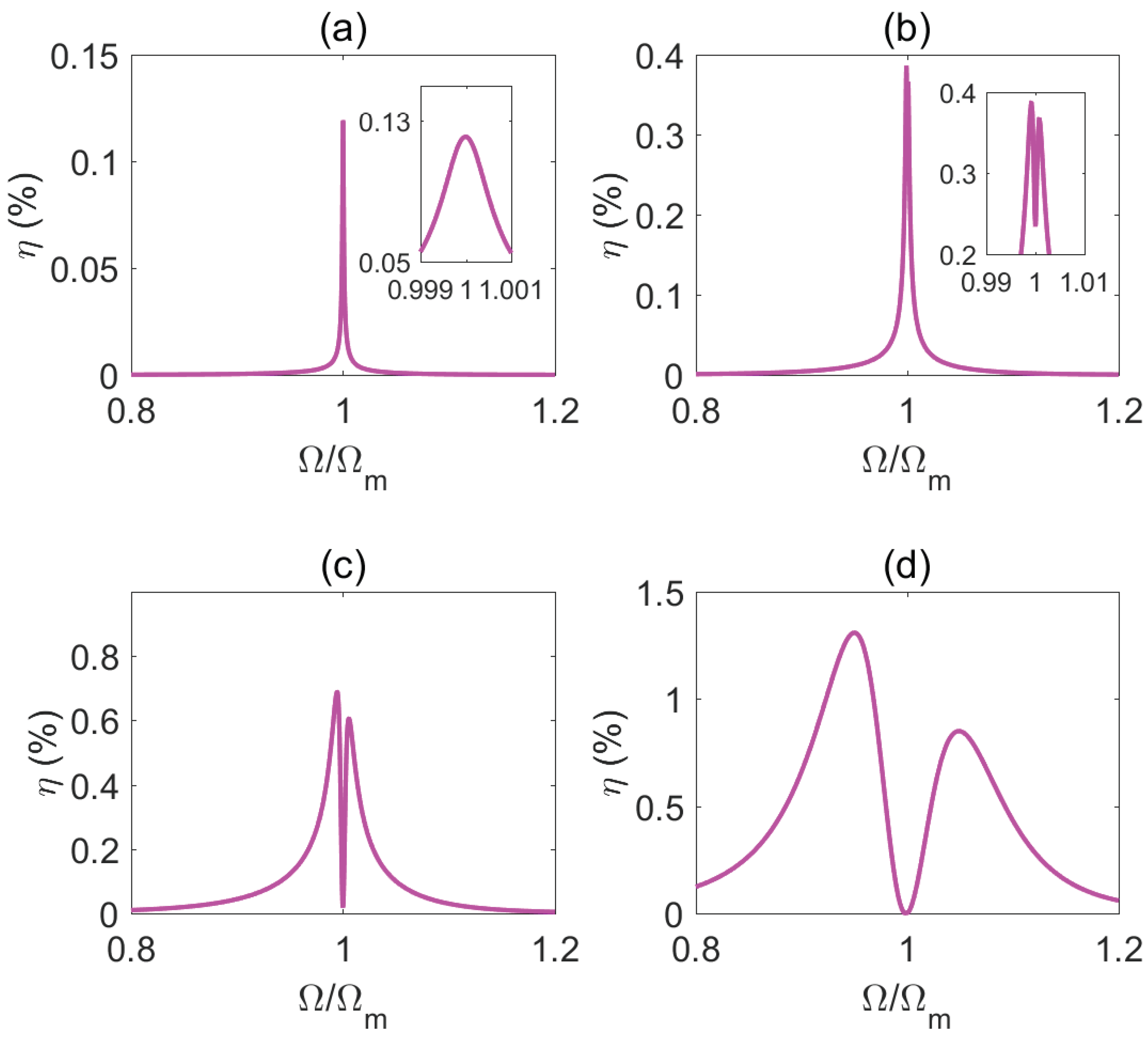
A high dependence of the efficiency of third-order sideband generation on the pumping field power is observed and more exact results are plotted in
Figure 3 by using the same experiment parameters [
13]. Due to the weakness of power of the control field (
= 0.1 mW), the efficiency of
is very low, about
under the condition
, as shown in
Figure 3a. Moreover, from the screenshot of
Figure 3a, we can see that there is not the optomechanically induced opacity of the third-order sideband, which means that most of the probe field is absorbed. As expected, the efficiency of
is enhanced when we increase the pumping field power.
Figure 3b shows that the efficiency of third-order sideband generation increases to about
in the case of the control field power
= 0.1 mW. Understandably, with the increase of the drive field power, the photon number of the intracavity field increases, and the nonlinear response of the system is also enhanced. Meanwhile, there is an opacity window near the resonance condition
, although it is not deep. The appearance of the opaque window can be explained by the splitting of the system energy level. On the one hand, when there is no control field, or the control field is weak, the coupling between the mechanical oscillator and the cavity field will form two dressed levels, and an obvious absorption peak will appear in the transmission spectrum under the resonance condition. On the other hand, when the power of the control field increases gradually, one of the dressed energy levels will be modified and energy-level splitting will occur, and the absorption peak will gradually disappear under the resonance condition, thus forming a transparent window, namely OMIT [
10]. At this time, there is not enough energy to stimulate the generation of the third-order sideband. Consequently, an opaque window will appear in the third-order sideband generation spectrum. To further enhance the efficiency of third-order sideband generation, we increase the power of the pumping field
= 1 mW, and the result is shown in
Figure 3c) It is clearly seen that the opacity window near the resonance condition
becomes distinct relative to the case in
Figure 3b. In addition, the efficiency of the third-order sideband
increases with the power of the driven field increasing and the maximum value of
is about
. Subsequently, we increase the control field power again to
= 10 mW, as shown in
Figure 3d. Visibly, we can see that not only the maximal efficiency of the third-order sideband increases to about
, but also the width of the opacity window increases significantly. Considering
Figure 2 and
Figure 3 together, if the power of the control field
is asthenic, OMIT will not appear in the output spectrum. In this case, around the resonance condition, i.e.,
, the transmission coefficient of the probe field is almost zero, which means that the probe field is almost completely absorbed. Meanwhile, the third-order sideband
achieves the maximum amplitude at the resonance condition
. However, when we increase the pumping field power, the transparent window takes place near the resonance condition
. From the above discussion, we can note that the efficiency of the third-order sideband is more sensitive than OMIT with the changes of the control field, whether it is the range of intensity changes, or the width of the opacity window. Based on this, we can use the effect of the nonlinear third-order sideband for more accurate precision measurement [
25,
27].
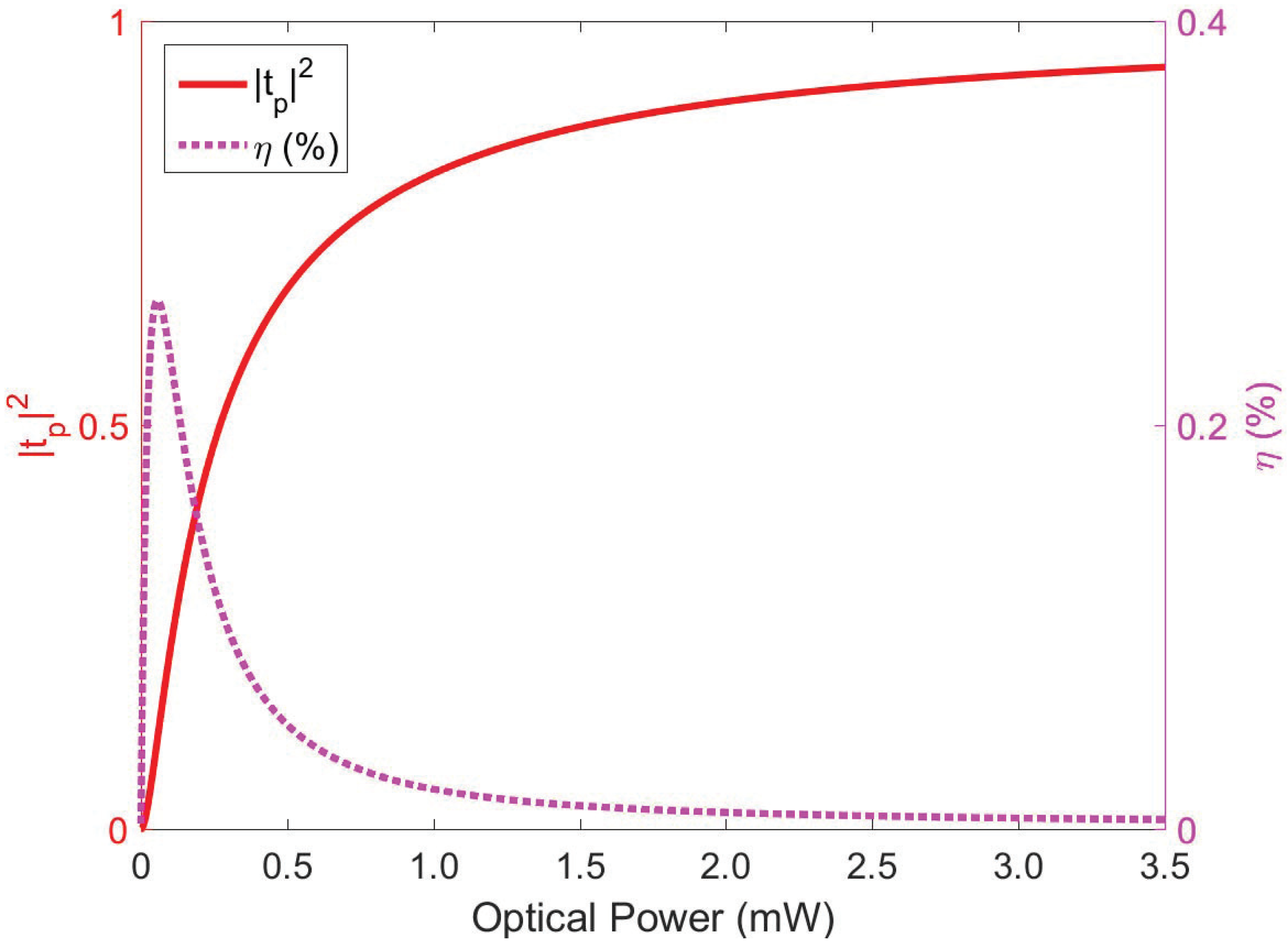
For more intuitive study of the influence of OMIT to the efficiency of the third-order sideband, the calculation results of
and
vary with the power of the control field at the resonance condition
and are plotted in
Figure 4. The red solid line represents the change of
varying with the control field and the pink dotted line represents the efficiency of third-order sideband generation. Clearly, we can see that
increases as the power of the control field increases, while the efficiency of third-order sideband
decreases rapidly after a rapid as well as brief increase, and finally tends to zero. More specifically, when the control field is weaker than about 0.1 mW,
increases sharply with the optical power of the control field and reaches its maximum at about
= 0.1 mW. For another case where the optical power of the control field is larger than 0.1 mW,
increases continuously and finally stabilizes while
decreases slowly and finally stabilizes quite low. The reason for this phenomenon is that under the action of a strong control field, the appearance of OMIT suppresses the generation of the third-order sideband under the resonance condition
.
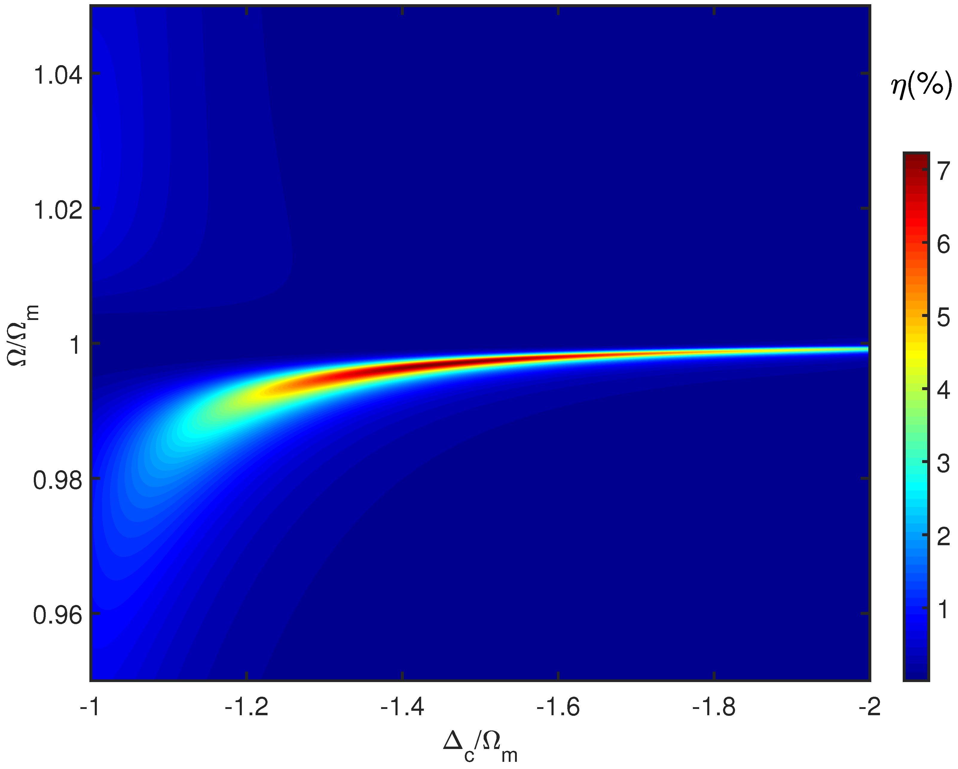
Up to now, we have mainly focused on the influence of OMIT on the third-order sideband generation. Now, however, we turn to discuss how to increase the amplitude of the third-order sideband by regulating the detuning between the cavity field and the control field
. The efficiency of the third-order sideband process
varies with the driving frequency
and the detuning
is plotted in
Figure 5. Here, the pumping field power used is
= 5 mW. In the case of
, the efficiency of the third-order sideband
is only about
, the same as in
Figure 2. With the change of the control field detuning, the amplitude of the third-order sideband has greatly increased. Specifically, the amplitude of the third-order sideband
increases to about
when the control field detuning is taken to
.
The effective amplitude of the third-order sideband reaches the maximum, about
, under the condition
. Further increasing the control field detuning, however, does not lead to a significant improvement; instead, there a slight decline, and the amplitude of the third-order sideband is stable around
under the resonance condition
. Interestingly, we observe that the relationship between
and the driving field frequency
appears to be totally different. More specifically, for the case of
, the effective amplitude of the third-order sideband is quite low and the change of the control field detuning
does not improve the effective amplitude of the third-order sideband. However, for the case of
, the effective amplitude of the third-order sideband increases as the control field detuning
increases. The physical mechanism can be understood as follows: the asymmetry of sideband distribution is caused by the constructive and destructive interference between the direct third-order sideband process and the upconverted first-order sideband process. Therefore, we can simultaneously adjust the driven frequency
and the control field detuning
, to achieve the largest amplitude of the third-order sideband rather than by relying on a strong laser drive [
46,
47].
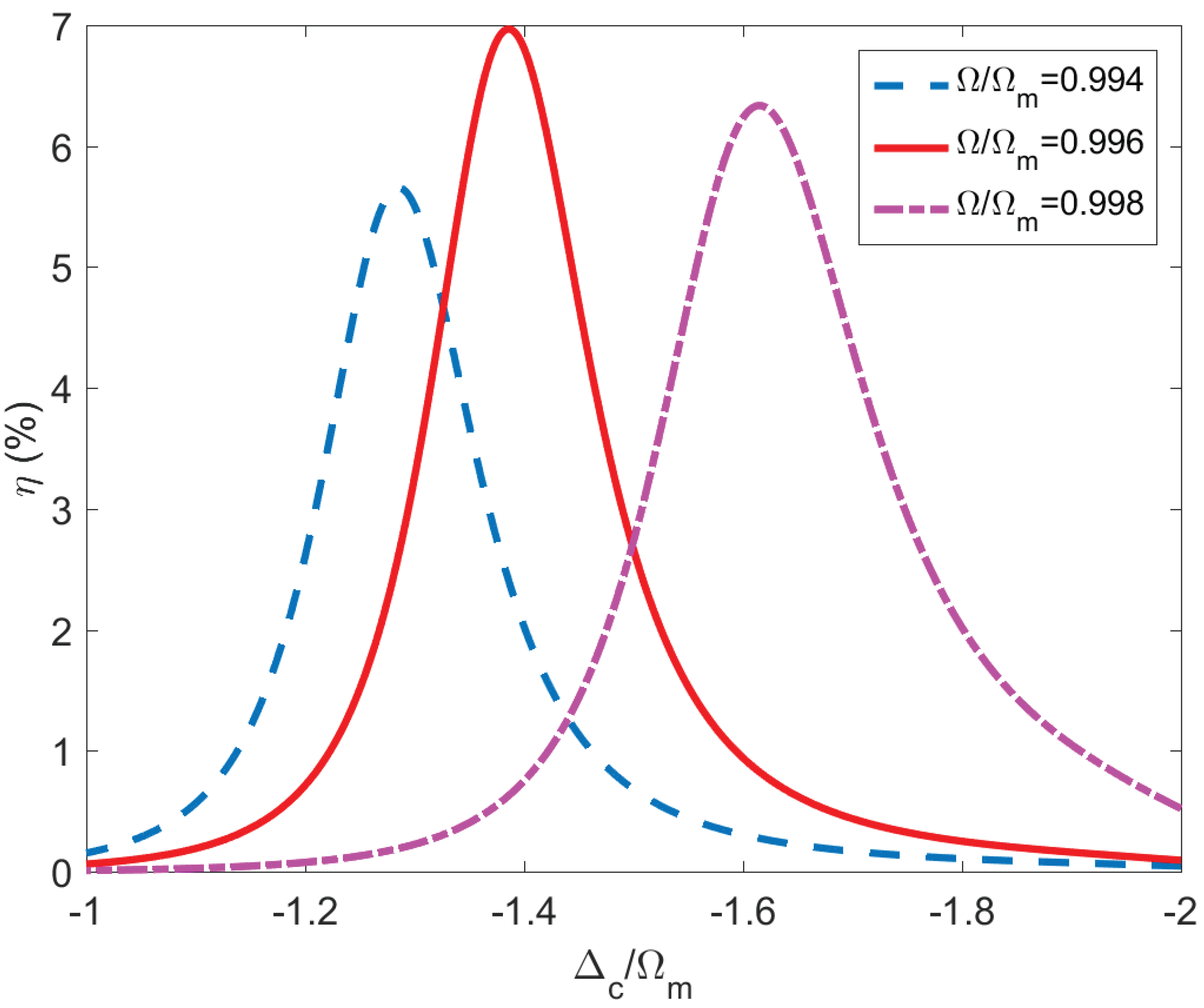
Due to the asymmetry of the third-order sideband generation around the resonance condition
, it is necessary for us to study the specific driven frequency
that satisfies the third-order sideband increase by adjusting the detuning
. As shown in
Figure 6, the blue dotted line represents the variation of the amplitude of the third-order sideband with the control field detuning
under the driven frequency
. We find that the efficiency of the third-order sideband
with the change of
satisfies the Lorentz-like distribution. As the blue dotted line shows, the effective amplitude of the third-order sideband increases with raising the detuning and reaches the maximum value, about
, under
. However, the efficiency
decreases when we continue to enhance the control field detuning
and tends to stablilize. Next, we consider another specific driving frequency
. The correlation between the process of the third-order sideband generation
and the detuning
is the same as
(the red solid line shows), and the maximum value of
is about
at
. Likewise, the same result as the pink dash-dotted line shows for
, and the maximal efficiency of the third-order sideband reaches
at
. The physical mechanism by which third-order sideband generation efficiency has a local minimum at resonance (
) can be understood as follows: the upconverted first-order sideband process is weak when the OMIT occurs and when the detuning
of the driving field was increased, one of the absorption peaks will consequently move. At that time, the efficiency of
will quickly reduce near the resonance condition
; thus, it results in a visible third-order sideband generation. From the above discussion, one can achieve the maximum values of the third-order sideband by regulating driven frequency
and detuning
in the practical application of precision measurement.


