Multi-Channel Visibility Distribution Measurement via Optical Imaging

Abstract

Calibration of the imaging environment is an important step in computational imaging research, as it provides an assessment of the imaging capabilities of an imaging system. Visibility is an important quantity reflecting the transparency of the atmosphere. Currently, transmissometers and optical scatterometers are the primary methods for visibility measurement. Transmissometers measure visibility along a single direction between the transmitter and receiver but encounter challenges in achieving optical alignment under long baseline conditions. Optical scatterometers measure the visibility within a localized area since they collect only a small volume of air. Hence, both transmissometers and optical scatterometers have limitations in accurately representing the visibility distribution of an inhomogeneous atmosphere. In this work, a multi-channel visibility distribution measurement via the optical imaging method is proposed and validated in a standard fog chamber. By calibrating the attenuation of infrared LED arrays, the visibility distribution over the entire field of view can be calculated based on the atmospheric visibility model. Due to the large angle of divergence of the LED, the need for optical alignment is eliminated. In further discussion, the key factors affecting the accuracy of visibility measurement are analyzed, and the results show that increasing the measurement baseline, increasing the dynamic range of the detector, and eliminating background light can effectively improve the accuracy of visibility measurement.

1. Introduction

Atmospheric visibility is an important quantity used to characterize the transparency of the atmosphere [1,2]. Visibility is closely related to weather conditions [3,4,5], and when weather phenomena such as rainfall, fog, or haze occur, the transparency of the atmosphere decreases and visibility deteriorates, which could lead to a serious impact on daily life and production activities. Measuring and reporting the visibility condition is not only used in daily meteorological monitoring but also widely applied in fields such as aviation [6], navigation [7,8], land transportation [9,10], military activities, etc. Existing visibility measurement techniques mostly enable measurements of specific regions or single links, limiting their effectiveness in cases of inhomogeneous atmospheric distributions. Therefore, accurate visibility measurement and forecast for a large scene is urgently needed.

The earliest method for visibility measuring was visual observation, but due to the subjective nature of human observers and the complexity of the environment, it was difficult to achieve high accuracy and objectivity [11]. As a result, instruments for visibility measuring were developed to replace the traditional human eye observation [12,13]. Currently, common instruments used for visibility measurement include transmissometers [14], optical scatterometers [15], and visibility LiDARs [16].

Transmissometer measures visibility by assessing the atmospheric transmittance between two points in space, it can achieve high accuracy in visibility measurement, but it only takes measurement along only one single direction between transmitter and receiver, and the installation and calibration could become challenging under long baseline conditions. Optical scatterometer estimates visibility by measuring the scattering effect within a small volume of air and has the advantages of low cost, small size, and easy installation, but it only measures within a localized area. Hence, both transmissometers and optical scatterometers measure visibility that is limited to a specific localized area, when the atmospheric distribution is inhomogeneous in a large scene, the measurement results have limitations in accurately describing the visibility distribution that is spatially varying. Visibility LiDARs measure visibility by assessing the backscattering effect of a large area in the atmosphere. Compared to other instruments, visibility LiDARs have a larger detection area, therefore yielding more representative measurements. However, they are limited in their capability to measure extremely low-visibility conditions and have the disadvantages of high cost, complex structure, and high technical difficulty.

To describe the inhomogeneous visibility distribution and enable simultaneous measurement of multiple regions in a large scene, a multi-channel visibility distribution measurement via optical imaging method is proposed in this work. Similar to a transmissometer, in this method, the visibility is measured by assessing the atmospheric transmittance, but instead of using a collimated beam and the photodetector, multiple LED arrays are utilized as the detected signal, while an optical imaging system as the detector. Since the infrared wavelength of light has a stronger ability to penetrate the fog, the Near-infrared LED arrays were utilized [17]. The measurement area of visibility would be determined by the field of view of the optical imaging system, which could be controlled by the sensor size of the camera and the focal length of the lens. The space between each LED array and the optical imaging system forms a measurement channel, by evenly distributing the LED arrays in the space, multiple measurement channels are formed [18]. For each channel, an average visibility value can be obtained, providing an assessment of the imaging capabilities of the system. Experiments were conducted in a standard fog chamber to validate the proposed method, and potential sources of measurement errors were analyzed in further discussions. The experimental results demonstrate that through the calibration of the atmospheric transmittance in each channel, a comprehensive description of visibility for the entire field of view can be achieved.

2. Principle and Method

2.1. Definition of Visibility

Visibility is defined as the greatest distance at which a black object can be identified against the horizon sky during daylight [11]. According to Koschmieder’s law, visibility can be expressed as:

$$V=-\frac{ln\epsilon }{\sigma }=-\frac{ln0.05}{\sigma }$$

(1)

where V is the visibility value; $\epsilon$ is the threshold of visual contrast that humans can distinguish the target from the background, setting at 0.05 [19]; $\sigma$ is the extinction coefficient indicating the transparency of the atmosphere. Equation (1) suggests that the key to visibility measurement is to obtain the value of the extinction coefficient $\sigma$.

Transmissometers estimate the extinction coefficient $\sigma$ by measuring the attenuation of a light signal over a distance of L in the air, which can be described by the Bouguer-Lambert law as follows:

$$\sigma =-{\displaystyle \frac{lnT}{L}}=-{\displaystyle \frac{ln(F_1/F_0)}{L}}$$

(2)

where $F_0$ is the initial luminous flux of the light signal, $F_1$ is the attenuated luminous flux received after traveling through a distance of L in the air, and T is the atmospheric transmission factor.

Combining Equations (1) and (2), it leads to:

$$V={\displaystyle \frac{ln0.05·L}{ln(F_1/F_0)}}$$

(3)

Equation (3) is the basic formula for a transmissometer.

The concept of visibility is established on measurements of the attenuation of green light at a wavelength of 550 nm [11,20], which corresponds to the peak sensitivity of the human eye. However, when visibility is measured using instruments, it is common for the wavelength $\lambda$ of the detected light signal to deviate from the green light. Consequently, a modification of the formula is required. The modified formula can be expressed as follows:

$$V={\displaystyle \frac{ln0.05·L}{\ln (F_1/F_0)}}{\left({\displaystyle \frac{{\lambda }_0}{\lambda }}\right)}^q$$

(4)

where ${\lambda }_0$ represents the wavelength of green light, which is 550 nm. $\lambda$ is the wavelength of the detected light signal, q is a coefficient related to the particle size distribution in the atmosphere [21] and needs to be calibrated during the experiments, a detailed discussion on the calibration will be given in the subsequent section.

Equation (4) demonstrates that to calculate the atmospheric visibility value, several data need to be obtained, including the transmission distance L of the light signal, the initial luminous flux $F_0$ of the detected light signal, the attenuated luminous flux $F_1$ of the light signal after it has traveled through a distance of L, the wavelength $\lambda$ of the signal, and the value of q.

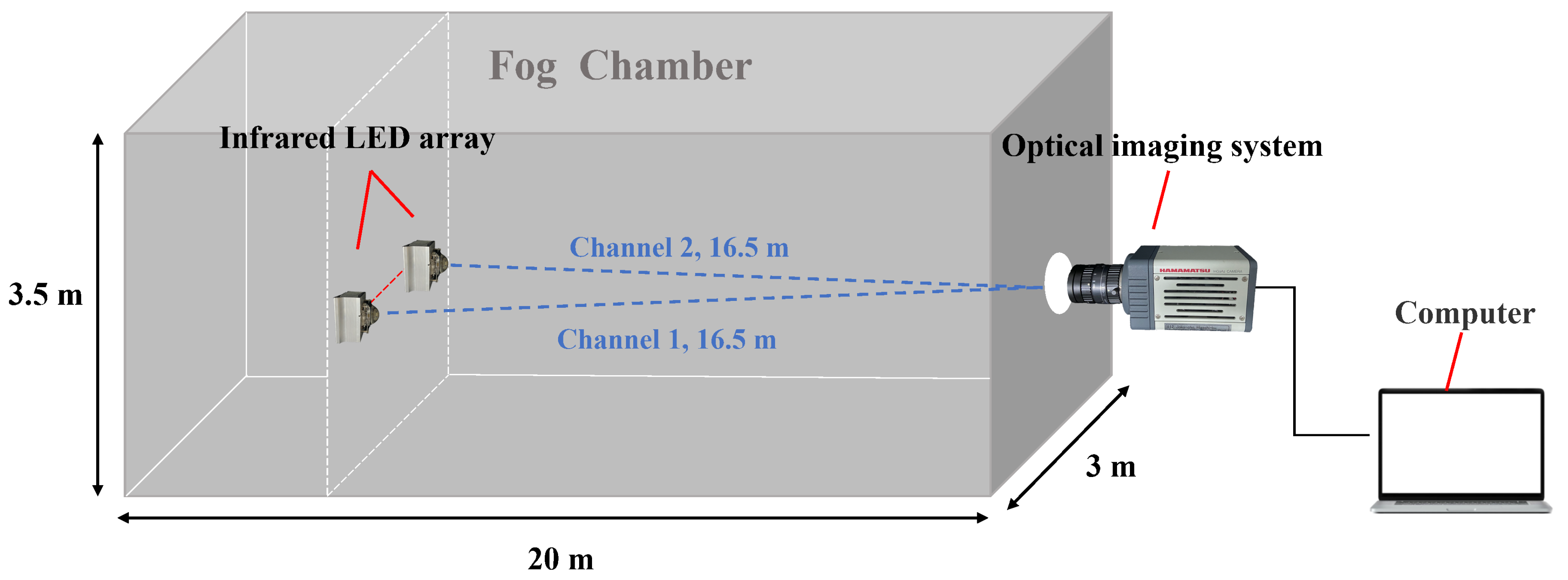
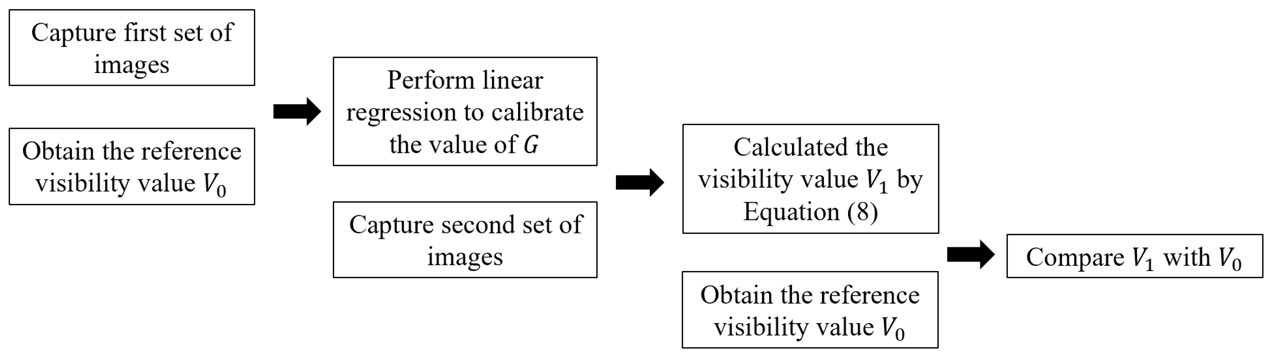
2.2. Experimental Methods

To validate the proposed visibility measurement method, a series of experiments were conducted in a standard fog chamber. The standard fog chamber has the dimensions of $20\times 3\times 3.5$${\mathrm{m}}^3$, and is in the Visibility Calibration Laboratory of China Meteorological Administration in Shanghai, China. The atmospheric visibility within the chamber is regulated by artificial fog generated with water mist particles, and the visibility value of the chamber is provided by the Vaisala PWD50, a forward-scattering visibility sensor, which would serve as the standard instrument in the calibration experiment of visibility measurement.

The visibility measuring system of the proposed method consists of three components: multiple infrared LED arrays, an optical imaging system, and a data processing module. The experimental setup is shown in Figure 1, two LED arrays were set inside the chamber serving as the detected light signal, and the optical imaging system outside the chamber to capture images of the LED arrays through an observation window. The LED arrays were directed towards the optical imaging system, with a distance of $L=16.5$ m (i.e., the baseline length), and the space between each array and the optical imaging system forms a visibility measurement channel individually.

The LED array light source utilized in the experiment is comprised of 50 LEDs, a lens with a divergence angle of 60${}^{\circ }$ and a diameter of 50 mm, and a heat sink of $80\times 80\times 96$ mm${}^3$. Each infrared LED array has an output power of 50 w, with a peak wavelength ${\lambda }_p$ of 1027 nm, and a full width at half maximum (FWHM) $\Delta \lambda$ of 37.6 nm. The optical imaging system consists of the Hamamatsu InGaAs Camera C14041-10U and a lens with a focal length of $f=50$ mm. The camera has a sensitivity wavelength range of 950 nm to 1700 nm, with a quantum efficiency of 60% within this wavelength range and a digital output of 14 bits.

The experiments were conducted according to the following procedure: the chamber was initially filled with fog, while the fog particles settled homogeneously, creating varying levels of visibility within the chamber. Images of the light signal were captured at different visibility levels, and the real-time visibility values of the chamber were obtained from the reference visibility meter, corresponding to the image acquisition time. The captured images were then processed to obtain the attenuation of the signal, and the visibility value could be calculated according to the atmospheric visibility model.

According to Equation (4), the calculation of atmospheric visibility requires certain parameters. These could be obtained from the data collected in the experiment.

First is the attenuation of the signal, which could be characterized by the intensity variation obtained from the images. The camera records the grayscale values of the image pixels. When the camera is appropriately adjusted and well-operated within a linear working region, there exists a linear relationship between the grayscale value of the signal pixel and the intensity of the signal [22]. Thus, the grayscale value of a pixel can serve as an indicator of the signal intensity, and the attenuation of the signal can be quantified by observing the corresponding decline in the grayscale value.

The method of obtaining the intensity of the light signal from the image is as follows: first, the pixel region of the light signal in the image is selected, as shown in Figure 2, then the grayscale values of this region are integrated, divided by the exposure time and the quantum efficiency to obtain the intensity of the signal per unit time. Denote the intensity value as I, this calculation can be expressed as follows:

$$I=\frac{{\sum }_i^n{R}_i}{T·\eta }$$

(5)

where n is the number of pixels occupied by the signal region, $R_i$ is the grayscale value of each pixel, T is the exposure time and $\eta$ is the quantum efficiency of the optical imaging system. During image acquisition, the exposure time T is adjusted based on the image histogram to ensure that the light signal area remains within the appropriate exposure range, ensuring the avoidance of overexposure while maximizing the value of $R_i$.

In practical measurements, the presence of background light captured by the camera along with the detecting light signal can introduce inaccuracies in light intensity measurements and subsequently affect the accuracy of visibility measurements. The background light in the standard fog chamber includes weak indoor lighting, slight transmission of outdoor sunlight, and light reflected from the inner wall of the chamber caused by the light signal. To accurately extract the intensity of the detected signal, all captured images were pre-processed to eliminate the influence of background light.

The method of background light elimination is as follows: First, the average intensity of a region in the image corresponding to a non-reflective black background in the chamber was calculated, denoted as $\overline{I_b}$. Then, the intensity value after background light elimination, denoted as $I^{\prime }$, can be obtained by subtracting the product of the number of pixels of signal, denoted as n, with the average background intensity $\overline{I_b}$ from the original light intensity value I. This calculation can be expressed as follows:

$$I^{\prime }=I-n\times \overline{I_b}$$

(6)

Denote the initial intensity of the light signal as $I_0$, and the attenuated intensity as $I_1$, Equation (4) can be written as follows:

$$V={\displaystyle \frac{ln0.05·L}{ln(I_1/I_0)}}{\left({\displaystyle \frac{{\lambda }_0}{\lambda }}\right)}^q$$

(7)

The initial intensity $I_0$ of the light signal can be approximated by the intensity value obtained from the image captured under high-visibility conditions. Assuming the permissible error for the initial intensity value $I_0$ is a%, the approximate intensity of the signal obtained from the image can be expressed as $I_1=I_0(1-\mathrm{a}\%)$, substitute it into Equation (7), the minimum visibility conditions required for capturing this image can be calculated.

According to Equation (7), the calculation of visibility also requires the value of q and the wavelength $\lambda$ of the detected signal. Some previous studies have conducted calibration to determine the value of q, in [23], q is given as the function of visibility, while in [21], the q value is re-calibrated and defined as the function of wavelength. To ensure the accuracy of the proposed method, the value of q needs to be re-calibrated on our measurement system. Furthermore, it should be noted that the detected light signal used in the experiment is emitted by LED arrays, which have a broad spectral distribution and poor monochromaticity. Thus, the precise value of the wavelength is uncertain in this system. Define the correction coefficient $G={\left(\frac{550}{\lambda }\right)}^q$, Equation (7) can be simplified:

$$V={\displaystyle \frac{ln0.05·L}{ln(I_1/I_0)}}·G$$

(8)

where G is the coefficient that needs to be calibrated.

The value of G can be determined through the following procedure:

A series of attenuated intensities $I_1$ are obtained from the captured images under various visibility conditions and the real-time visibility value of the chamber $V_0$ is obtained from the reference visibility meter based on the time of image acquisition. Subsequently, a linear regression analysis is conducted with $V_0$ on the vertical axis and $ln0.05$·$L/[ln(I_1/I_0)]$ on the horizontal axis. If the regression analysis demonstrates a linear relationship, the visibility measurement model is validated, and the slope of the linear equation represents the value of the correction coefficient G.

To validate the proposed method and evaluate the accuracy of the measurement, two sets of experiments were conducted. The overall process of experiments is shown in Figure 3.

The first set of experiments aims at verifying the feasibility of the measurement model and calibrating the correction coefficient. A set of images was captured under different visibility conditions, and a linear regression analysis was performed on the attenuated light intensity values obtained from these images, along with the corresponding output values from the reference visibility meter to calibrate the value of G.

The second set of experiments aims at evaluating the accuracy of the visibility measurement method. Another set of images was captured using the same method to obtain the attenuated intensity. These intensity values, along with the value of G calibrated from the first experiment, were utilized in the measurement model to calculate the visibility of the chamber. The calculated results were then compared with the reference visibility values, and the measurement errors were further analyzed.

3. Results and Analysis

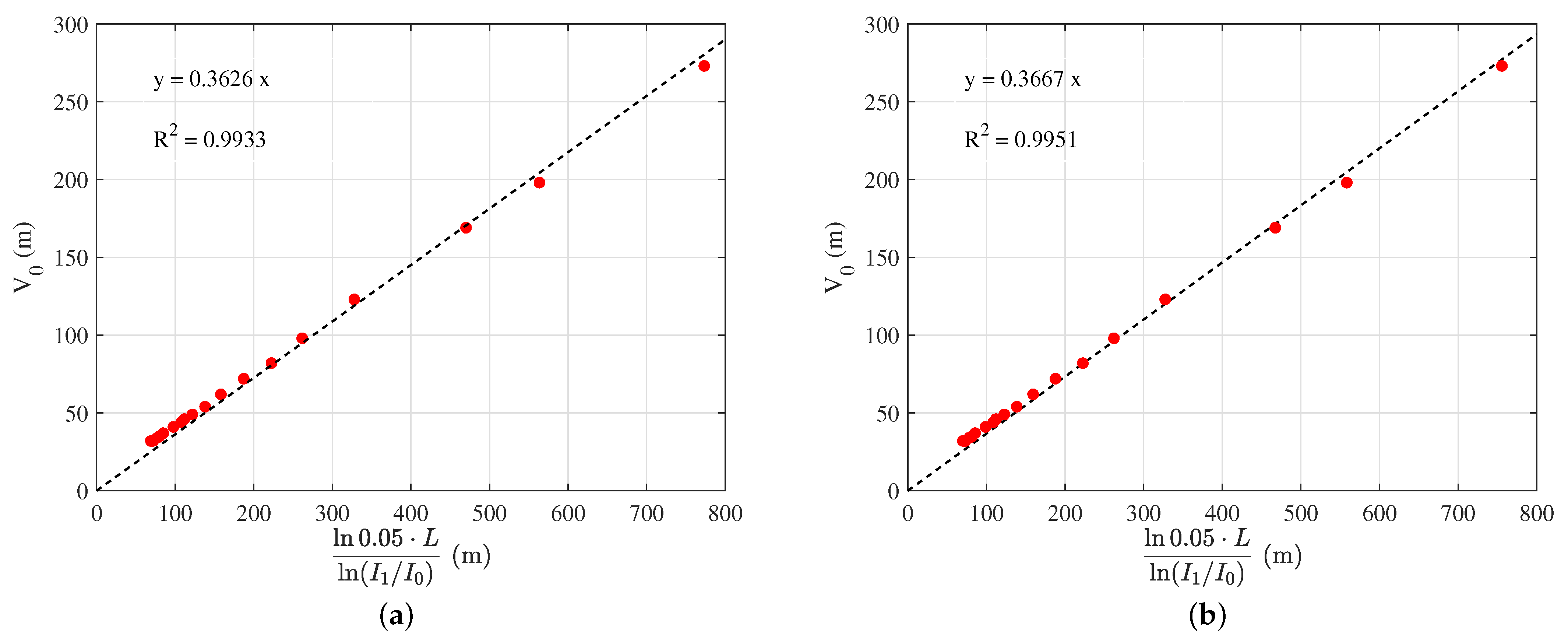
3.1. Coefficient Calibration

Two distinct visibility measurement channels were established in the chamber. Hence, coefficient calibration was conducted separately for each channel. As discussed in Section 2.2, the first set of images under different visibility conditions were captured to obtain a series of attenuated intensity $I_1$. An image was captured when the visibility in the chamber reached 1.13 km to obtain the approximation of initial intensity $I_0$ of the signal. The results of linear regression are presented in Figure 4.

As depicted in Figure 4, the coefficient of determination, $R^2$, for the data obtained from Channel 1 is 0.9933, while for Channel 2, it reaches 0.9951. The high value of $R^2$ indicates a strong fit of the regression model to the experimental data, therefore confirming the feasibility of the measurement model. The value of the correction coefficient for each channel is summarized in

Table 1. The wavelength correction coefficients of each channel.

	Channel 1	Channel 2
G	0.3626	0.3667

.

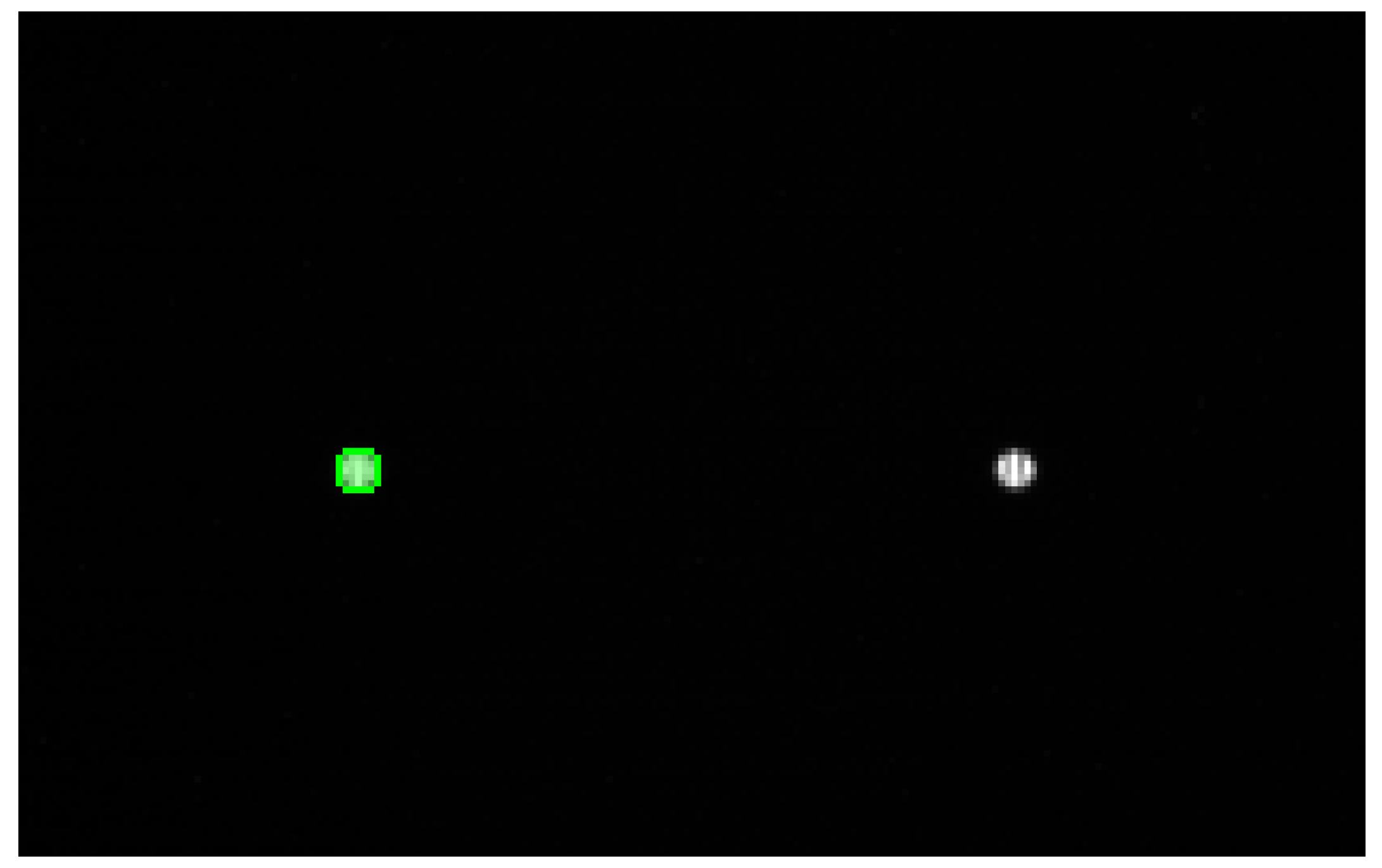
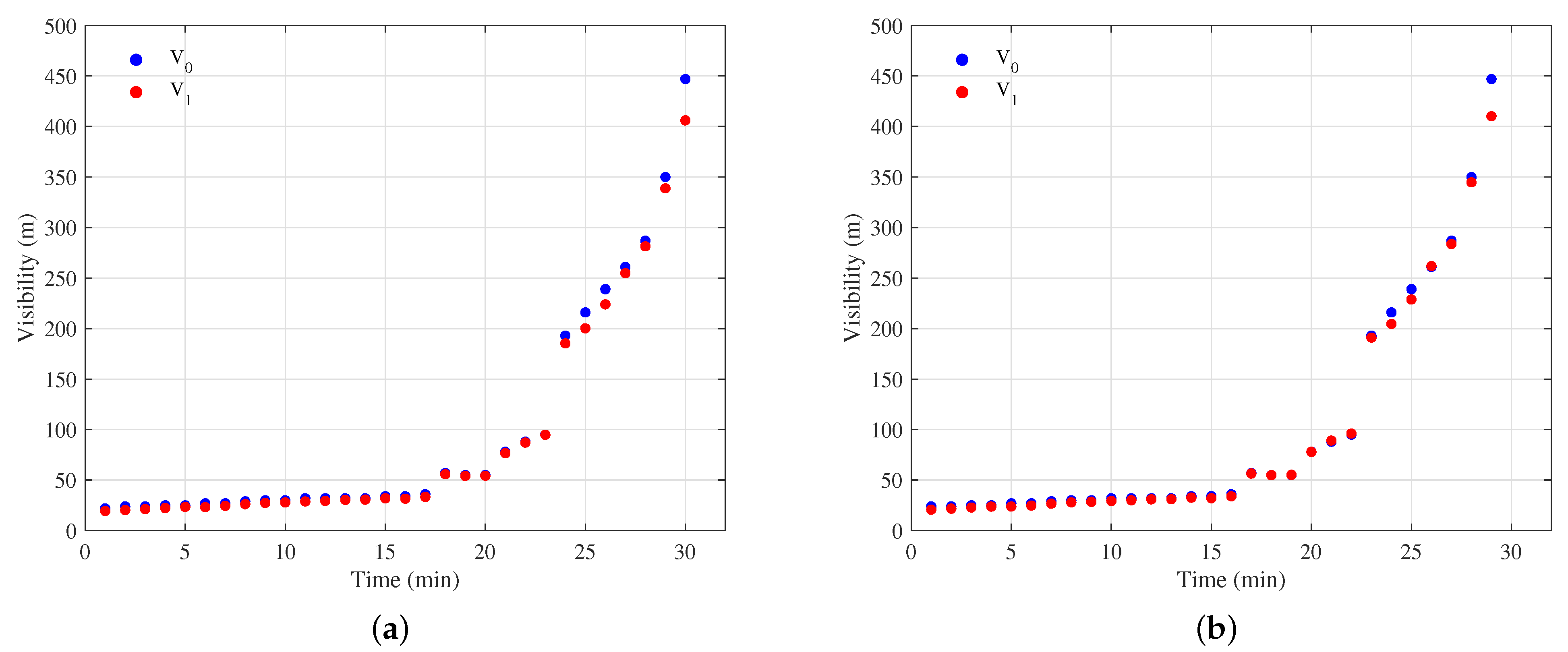
3.2. Data Processing

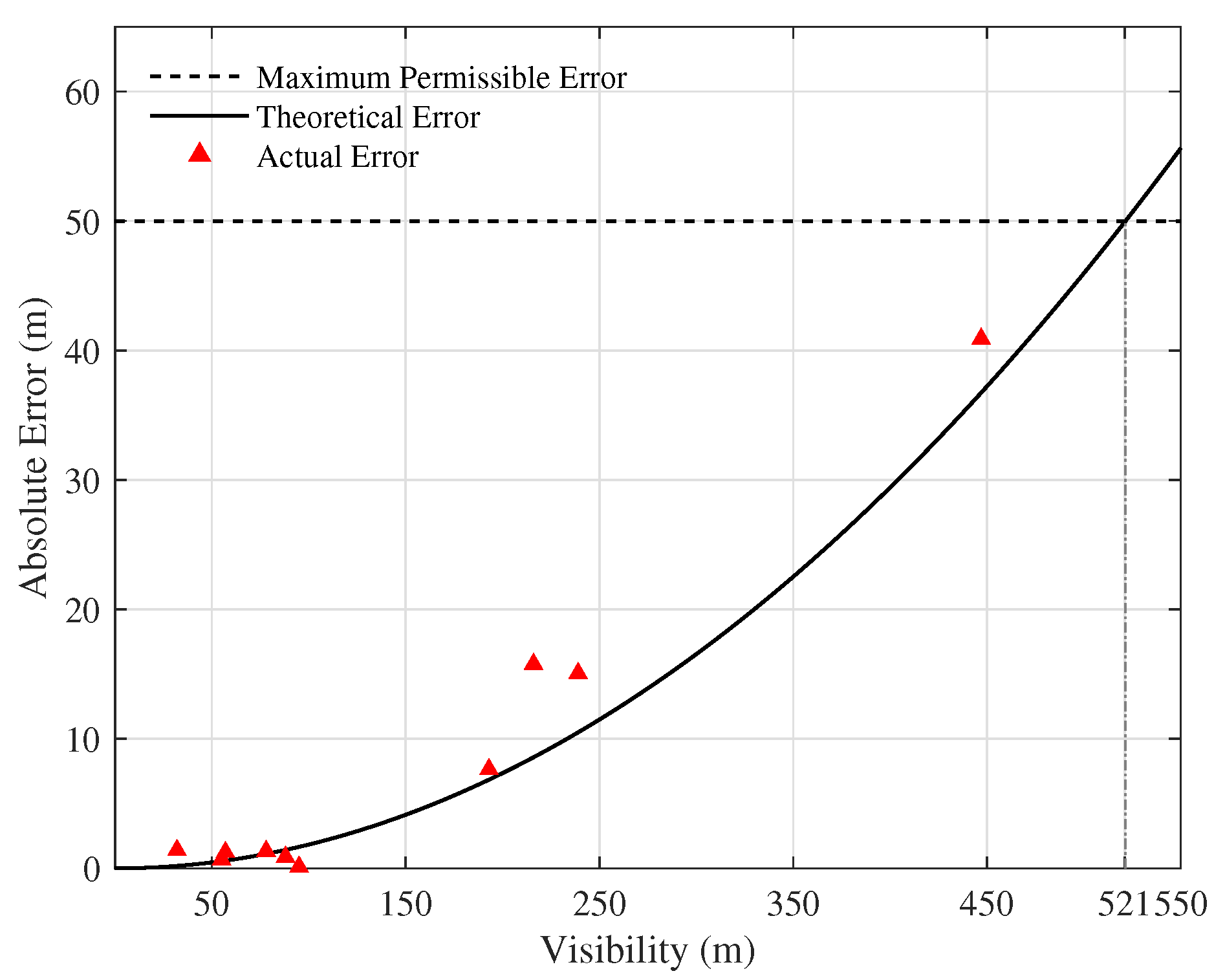
The strong linear correlation in the regression results validates the measurement model. To evaluate the accuracy of the method, another set of light signal images was collected. Substituting $I_1$ and $I_0$ into Equation (8) along with the previously calibrated coefficient G in Section 3.1, the visibility value $V_1$ could be calculated. The calculated results $V_1$ were then compared with the reference data $V_0$ in Figure 5.

Denote the absolute error of the measurement results as $\Delta V$, $\Delta V$ can be calculated as follows:

$$\Delta V=|V_1-V_0|$$

(9)

According to the ’Test Method for Forward-Scattering Visibility Meter’ published by the China Meteorological Administration (CMA) [24], the maximum permissible indication error for a visibility meter is $\Delta V=\pm 50$ m for $V\le 500$ m. The experimental data show that the absolute error range for Channel 1 is within $\Delta V_1\in [0.12,40.90]$ m, and for Channel 2 is within $\Delta V_1\in [0.01,36.79]$ m, both fall within the permissible error range.

As depicted in Figure 5, it is evident that for low-visibility conditions (V < 100 m), the experimental results $V_1$ closely align with the reference value $V_0$. However, as the visibility of the chamber increases, a noticeable divergence emerges between these two datasets, indicating an increasing measurement error.

3.3. Error Analysis

To improve the measurement accuracy, the source of measurement errors would be discussed in this section. For the optical imaging system, when scene radiation enters the sensor, noise is inevitably introduced during the subsequent processing of the output image. Various sources of noise can contribute to deviations between the output values and the true values.

Hence, the error introduced by noise in the visibility measurement would be considered, which could be calculated as follows:

$${\sigma }_V=\sqrt{{\left(\frac{\partial V}{\partial I_1}\right)}^2{\sigma }_{I_1}^2+{\left(\frac{\partial V}{\partial I_0}\right)}^2{\sigma }_{I_0}^2}$$

(10)

Substitute $I_1=\frac{{\sum }_i^n{R}_{1i}}{T_1·\eta }$ and $I_0=\frac{{\sum }_i^n{R}_{0i}}{T_0·\eta }$ into Equation (10) yields the following results:

$${\sigma }_V=\frac{\sqrt{2}{V}^2}{-ln0.05·GL}·\frac{{\sigma }_{R_i}}{R_i}$$

(11)

where ${\sigma }_{R_i}$ is the readout noise of the optical imaging system, $R_i$ is the full-well capacity. For the Hamamatsu InGaAs Camera C14041-10U, its full-well capacity is 600,000 e⁻ and the readout noise is approximately 300 e⁻, resulting in ${\sigma }_{R_i}/R_i=1/2000$. The relationship between measurement errors and visibility is shown in Figure 6. It can be seen that as the visibility increases, the measurement error will become larger and larger due to the readout noise from the optical imaging system. Based on the standard published by CMA, the maximum permissible error for visibility measurement is set to $\Delta V=\pm 50$ m, so the upper range value of the visibility measurement could reach $V_{max}=521$ m for a baseline length of $L=16.5$ m.

Learning from Equation (11), to improve the accuracy of the proposed method and extend the measurement range, the measurement error can be reduced by increasing the value of L, $R_i$ or decreasing the value of ${\sigma }_{R_i}$.

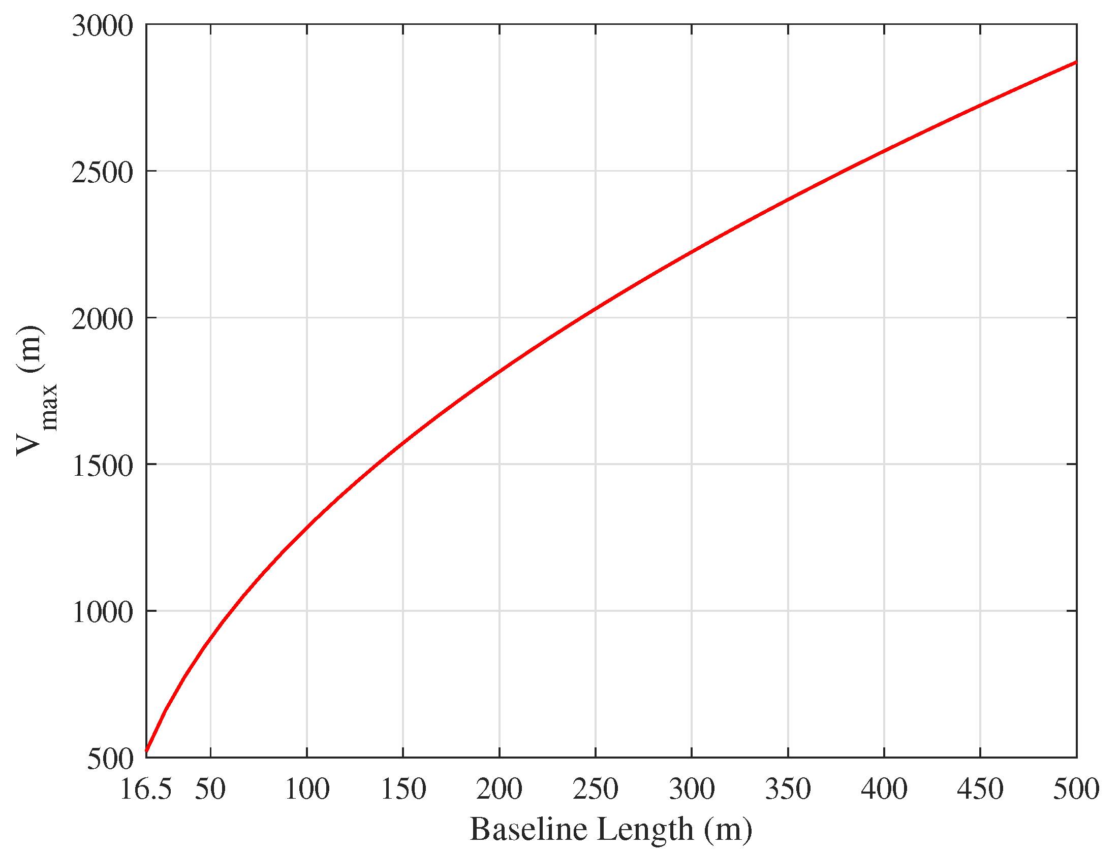
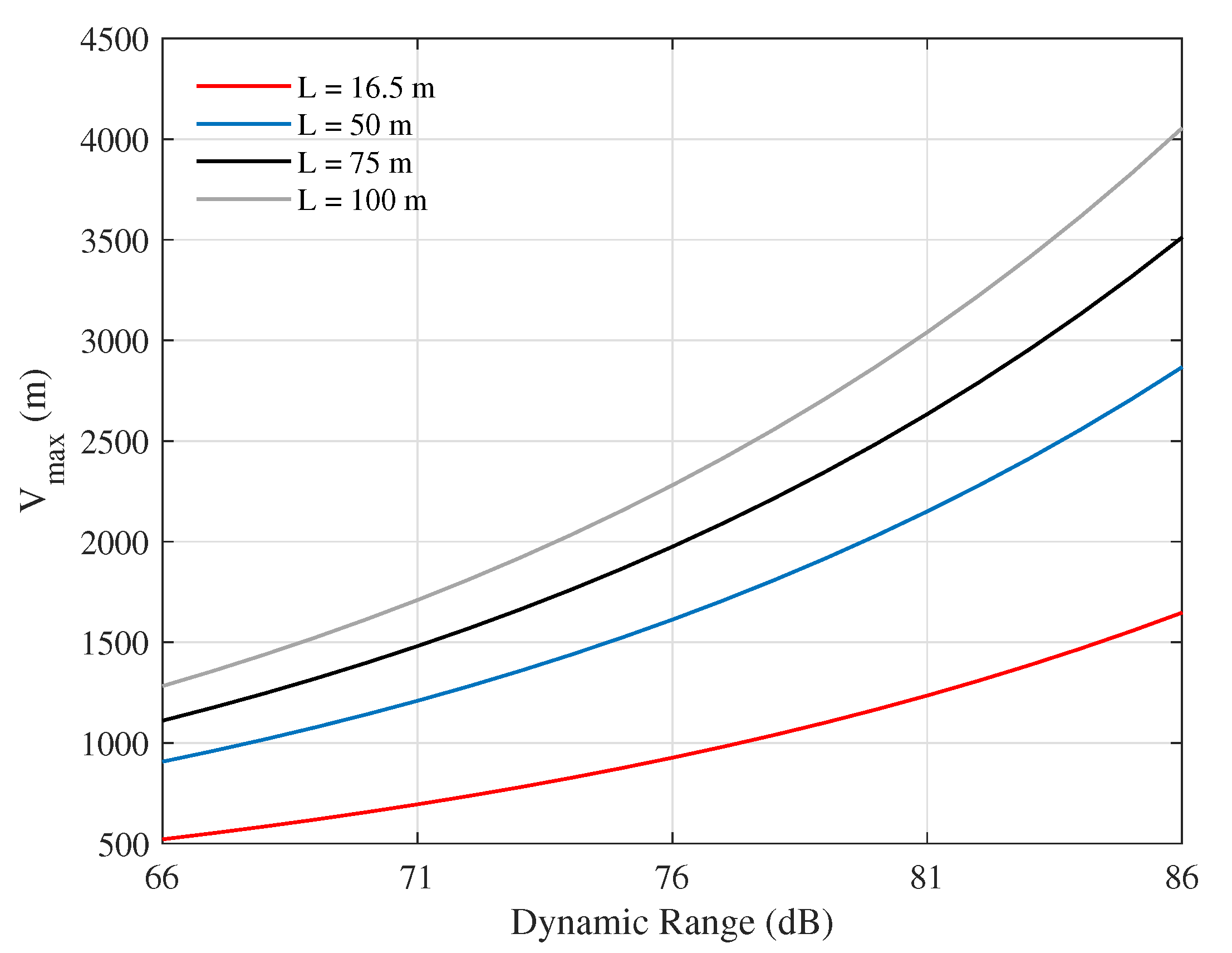
3.4. Discussion on Measurement Limitations

To assess the limitations of the measurement, theoretical calculations of the effects of various factors were performed and are discussed further in the following section. Figure 7 shows the relationship between baseline length and the upper range value of visibility measurement, it can be observed that as the baseline length increases, the upper range value of the measurement also increases.

The dynamic range of a camera is defined as the ratio of the full-well capacity to the readout noise, so Equation (11) can also be expressed as:

$${\sigma }_V=\frac{\sqrt{2}{V}^2}{-ln0.05·GL}·\frac{1}{DR}$$

(12)

The relationship between the dynamic range of the optical imaging system and the upper range value of the measurement under different baseline lengths is depicted in Figure 8. It can be observed that as the dynamic range of the optical imaging system increases, the measurement error decreases, increasing the upper range value of the measurement.

The impact of the dynamic range can be interpreted from the following perspective: the dynamic range represents the ratio of the highest to the lowest signal intensity, and it sets a limit on the accuracy of the data recorded by the detector. When the variation of the signal intensity falls below the threshold determined by the dynamic range, the optical imaging system fails to detect this variation, thus bringing high measurement errors.

For Equation (8), take the derivative of V with respect to $I_1$, we obtain:

$$dI=\frac{-ln0.05·GL·I}{V^2}dV$$

(13)

Equation (13) represents the variation in signal intensity $dI$, when there is a small change in visibility $dV$, for an experimental setup with a baseline length of L and a visibility level at V. As the visibility increases, the variation in signal intensity caused by attenuation becomes increasingly insignificant, making it challenging to detect. Thus, raising the dynamic range of the imaging system can significantly raise the upper range value of the measurement, and this is attributed to the improved ability of the system to detect more subtle changes in intensity information.

According to the discussion above, in addition to improving the system’s ability to detect subtle variation, the upper range value can also be raised by increasing the variation in signal intensity at high visibility. Learning from Equation (13), this could be achieved by increasing the baseline length L, or increasing the intensity of the detected signal I.

In summary, to enhance the measurement accuracy, improvements can be made by increasing the baseline length, the dynamic range of the optical imaging system, and the intensity of the detected signal.

The experimental results obtained within the standard fog chamber have provided strong validation for the proposed method. In future work, the proposed visibility measurement method will be applied in more complex environments. To improve the accuracy of the measurement, further experiments will be conducted utilizing imaging devices with higher dynamic range at a longer baseline. In addition, our experimental procedures will also be improved. A modulated signal will be introduced into the light source to effectively eliminate the background interference light in the images. Furthermore, data acquisition methods will be optimized to minimize unnecessary errors.

4. Conclusions

To describe the visibility of a field with inhomogeneous atmospheric distribution, a multi-channel visibility distribution measurement via optical imaging was proposed and tested in this work. By capturing the images of the infrared LED arrays and calibrating the extinction coefficient of each imaging channel, the visibility distribution for the entire field could be calculated. Based on the comparison tests in the standard visibility fog chamber, the validity of the measurement method was verified, and the sources of measurement errors were further analyzed. The effect of factors such as the length of the baseline and the dynamic range of the imaging device on the measurement range of this method was also calculated. Both the experimental results and the theoretical calculations show that the measurement results have high accuracy under low-visibility conditions, and the data errors increase as visibility rises. To reduce the errors, methods such as introducing modulated light sources, increasing the intensity of the light sources, increasing the length of the imaging baseline, optimizing the data acquisition methods, and improving the dynamic range of the imaging equipment can be taken to improve the accuracy of the measurement. In addition, it is important to note that due to the limitation of the measurement range, this method is better suited for low-visibility measurements.

References

1. Horvath, H. Atmospheric visibility. Atmos. Environ. (1967) 1981, 15, 1785–1796. [Google Scholar] [CrossRef]
2. Kim, K.W. The comparison of visibility measurement between image-based visual range, human eye-based visual range, and meteorological optical range. Atmos. Environ. 2018, 190, 74–86. [Google Scholar] [CrossRef]
3. Appel, B.; Tokiwa, Y.; Hsu, J.; Kothny, E.; Hahn, E. Visibility as related to atmospheric aerosol constituents. Atmos. Environ. (1967) 1985, 19, 1525–1534. [Google Scholar] [CrossRef]
4. Lee, C.G.; Yuan, C.S.; Chang, J.C.; Yuan, C. Effects of aerosol species on atmospheric visibility in Kaohsiung city, Taiwan. J. Air Waste Manag. Assoc. 2005, 55, 1031–1041. [Google Scholar] [CrossRef] [PubMed]
5. Charlson, R.J. Atmospheric visibility related to aerosol mass concentration. Environ. Sci. Technol. 1969, 3, 913–918. [Google Scholar] [CrossRef]
6. Leung, A.C.; Gough, W.A.; Butler, K.A. Changes in fog, ice fog, and low visibility in the Hudson Bay Region: Impacts on aviation. Atmosphere 2020, 11, 186. [Google Scholar] [CrossRef]
7. Chung, W.; Kim, S.; Choi, M.; Choi, J.; Kim, H.; Moon, C.B.; Song, J.B. Safe navigation of a mobile robot considering visibility of environment. IEEE Trans. Ind. Electron. 2009, 56, 3941–3950. [Google Scholar] [CrossRef]
8. Cai, C.; Gao, Y. A combined GPS/GLONASS navigation algorithm for use with limited satellite visibility. J. Navig. 2009, 62, 671–685. [Google Scholar] [CrossRef]
9. Huang, S.C.; Chen, B.H.; Cheng, Y.J. An efficient visibility enhancement algorithm for road scenes captured by intelligent transportation systems. IEEE Trans. Intell. Transp. Syst. 2014, 15, 2321–2332. [Google Scholar] [CrossRef]
10. Yang, L.; Muresan, R.; Al-Dweik, A.; Hadjileontiadis, L.J. Image-based visibility estimation algorithm for intelligent transportation systems. IEEE Access 2018, 6, 76728–76740. [Google Scholar] [CrossRef]
11. WMO. Guide to Instruments and Methods of Observation. Volume I: Measurement of Meteorological Variables; WMO: Geneva, Switzerland, 2020. [Google Scholar]
12. Luckiesh, M.; Moss, F.K. Visibility: Its measurement and significance in seeing. J. Frankl. Inst. 1935, 220, 431–466. [Google Scholar] [CrossRef]
13. Beuttell, R.; Brewer, A. Instruments for the measurement of the visual range. J. Sci. Instrum. 1949, 26, 357. [Google Scholar] [CrossRef]
14. Redmond, H.E.; Dial, K.D.; Thompson, J.E. Light scattering and absorption by wind blown dust: Theory, measurement, and recent data. Aeolian Res. 2010, 2, 5–26. [Google Scholar] [CrossRef]
15. Liu, W.T. Progress in scatterometer application. J. Oceanogr. 2002, 58, 121–136. [Google Scholar] [CrossRef]
16. Miclea, R.C.; Dughir, C.; Alexa, F.; Sandru, F.; Silea, I. Laser and LIDAR in a system for visibility distance estimation in fog conditions. Sensors 2020, 20, 6322. [Google Scholar] [CrossRef] [PubMed]
17. Shui, Y.; Zhou, J.; Huang, Y.; Shen, X.; Chen, L.; Chu, J.; Luo, X.; Liu, Y. Near-Infrared Imaging Optical Visibility Measurement System and Method. Chinese Patent Publication No. CN115326748A, 11 November 2022. [Google Scholar]
18. Li, M.; Fan, D.Q.; Yin, C.Y. Study on corresponding relation of laser and infrared transmittivity for smoke screen. J. Infrared Millim. Waves 2006, 25, 127–130. [Google Scholar]
19. International Civil Aviation Organization. Meteorological Service for International Air Navigation; International Civil Aviation Organization: Montreal, QC, Canada, 1976. [Google Scholar]
20. Schnapf, J.; Kraft, T.; Baylor, D. Spectral sensitivity of human cone photoreceptors. Nature 1987, 325, 439–441. [Google Scholar] [CrossRef] [PubMed]
21. Ijaz, M.; Ghassemlooy, Z.; Pesek, J.; Fiser, O.; Le Minh, H.; Bentley, E. Modeling of fog and smoke attenuation in free space optical communications link under controlled laboratory conditions. J. Light. Technol. 2013, 31, 1720–1726. [Google Scholar] [CrossRef]
22. Ma, S.; Xu, F.E.; Jietai, M.A.; Liu, D.; Zhang, C.; Ling, Y.; Zhen, X. Experimental Research on Visibility Reference Standard for Blackbody Targets. J. Appl. Meteorol. Sci. 2014, 25, 129–134. [Google Scholar]
23. Kim, I.I.; McArthur, B.; Korevaar, E.J. Comparison of laser beam propagation at 785 nm and 1550 nm in fog and haze for optical wireless communications. In Optical Wireless Communications III; SPIE: Bellingham, WA, USA, 2001; Volume 4214, pp. 26–37. [Google Scholar]
24. CMA. Test Method for Forward Scattering Visibility Meter; CMA: Beijing, China, 2020. [Google Scholar]
Figure 1. The experimental setup of the multi-channel visibility distribution measurement via optical imaging method. Two measurement channels were formed in the experiment, both with a baseline length of L = 16.5 m.
Photonics 10 00945 g001
Figure 2. One of the captured grayscale images of the LED arrays in the experiments, the area circled in green represents the pixel region of one array, occupying a total of 45 pixels.
Photonics 10 00945 g002
Figure 3. Overall process of experiments.
Photonics 10 00945 g003
Figure 4. The results of linear regression: (a) The results of Channel 1; (b) The results of Channel 2.
Photonics 10 00945 g004
Figure 5. Comparison of the calculated value V 1 with the reference value V 0 of visibility: (a) The data from Channel 1; (b) The data from Channel 2.
Photonics 10 00945 g005
Figure 6. The relationship between absolute measurement error and visibility for the system, with the solid black line corresponding to the theoretical error, the red dot corresponding to the actual error, and the dashed black line corresponding to the maximum permissible error. For a baseline length of L = 16.5 m, the upper range value of visibility measurement reaches V m a x = 521 m.
Photonics 10 00945 g006
Figure 7. Relationship between the length of the imaging baseline and the upper range value of the measurement.
Photonics 10 00945 g007
Figure 8. Relationship between the dynamic range and the upper range value of measurement under different baseline lengths.
Photonics 10 00945 g008