Simple Method of Light Field Calculation for Shaping of 3D Light Curves

 ,
, 
Abstract
:1. Introduction
2. Methods
2.1. Shaping of Parametric Light Curves: Theoretical Foundations
2.1.1. Formation of a Set of Light Points
2.1.2. Formation of Parametrically Specified Light Curves
2.1.3. Leveling the Intensity on the Curve by Taking into Account Singular Points (Cusps)
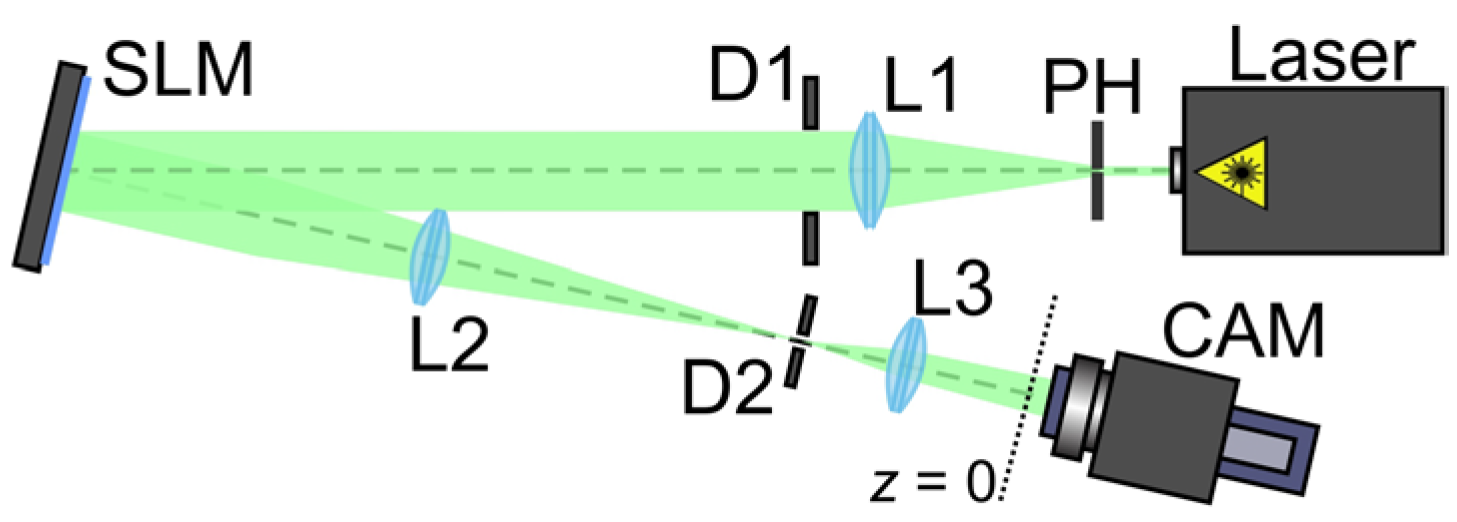
2.2. Experimental Setup
3. Results
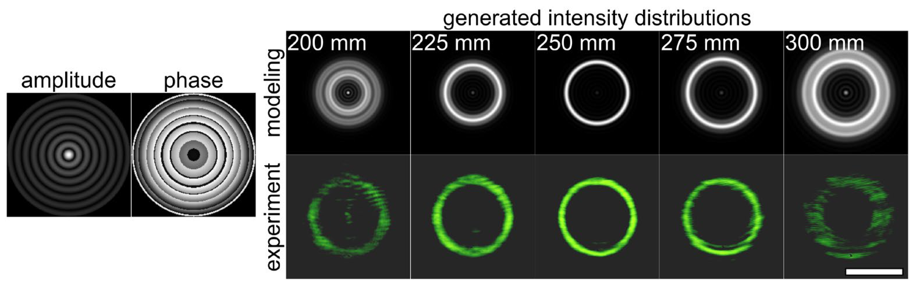
3.1. Light Ring
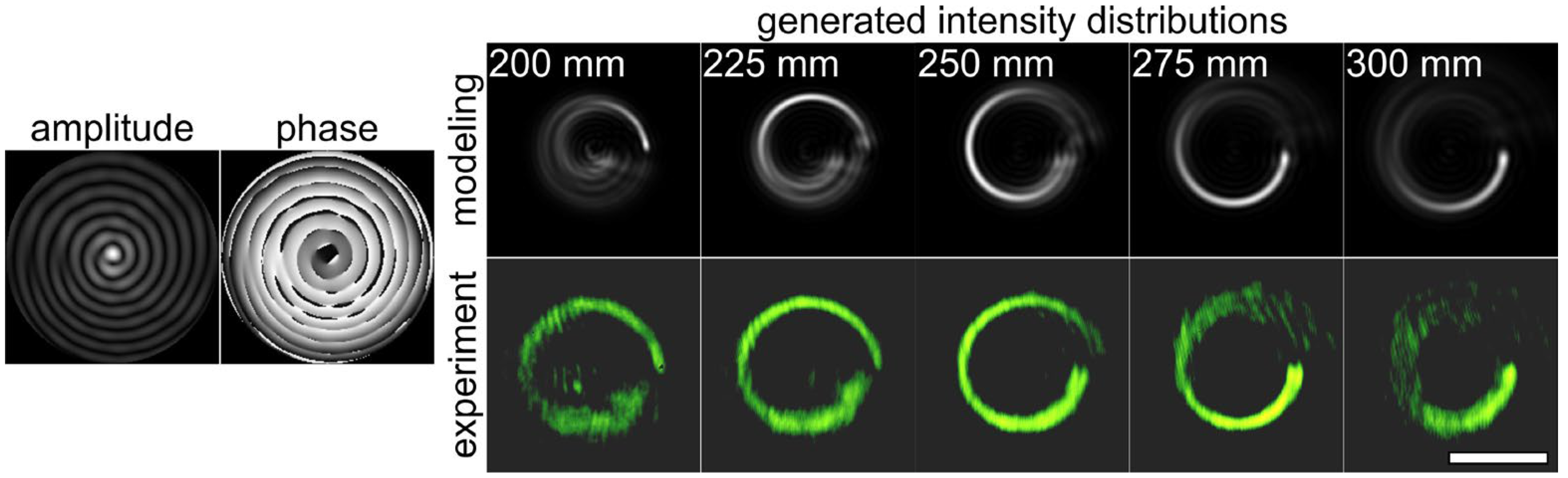
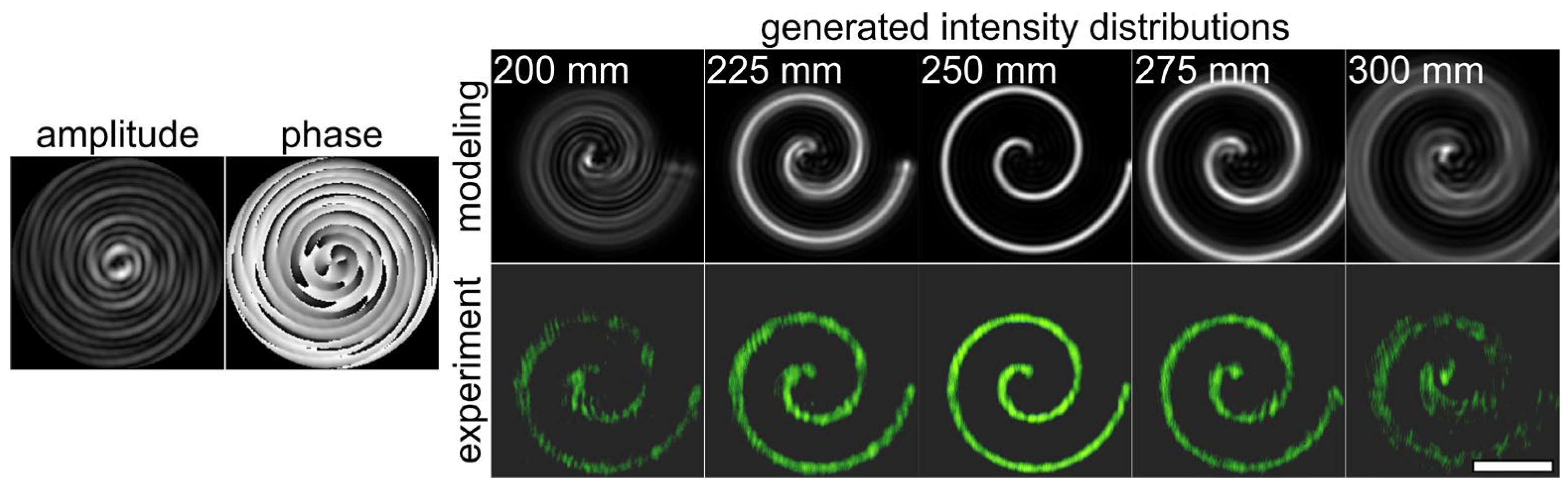
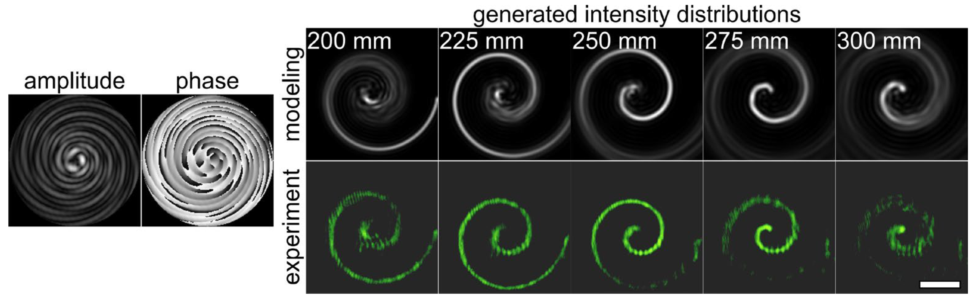
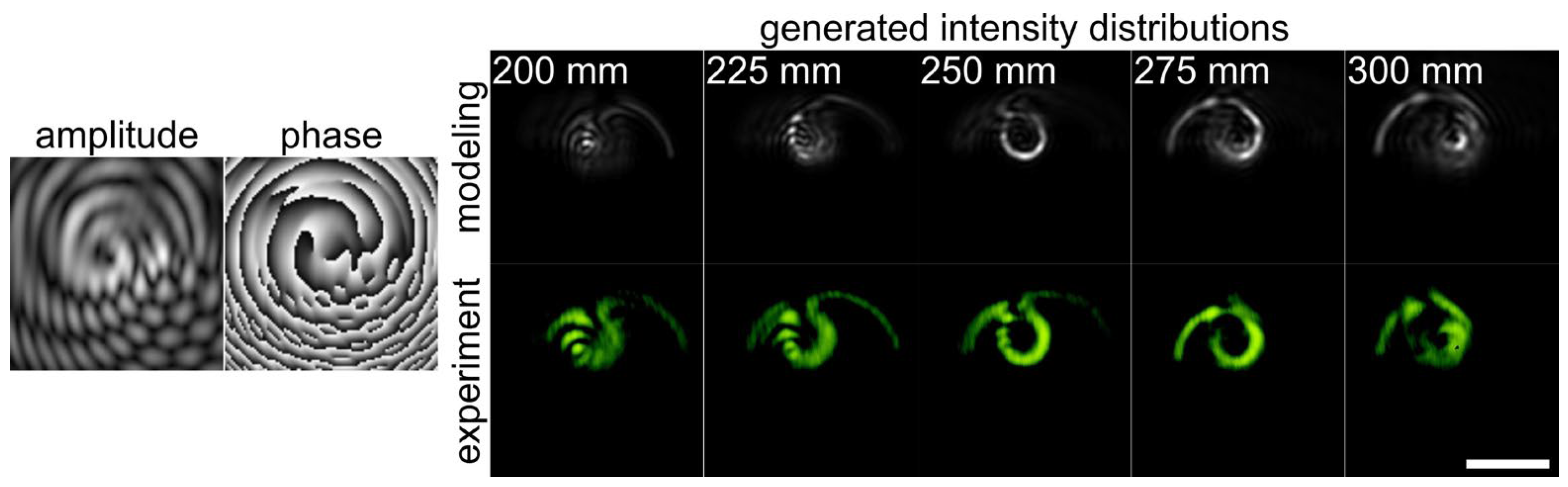
3.2. Light Spiral
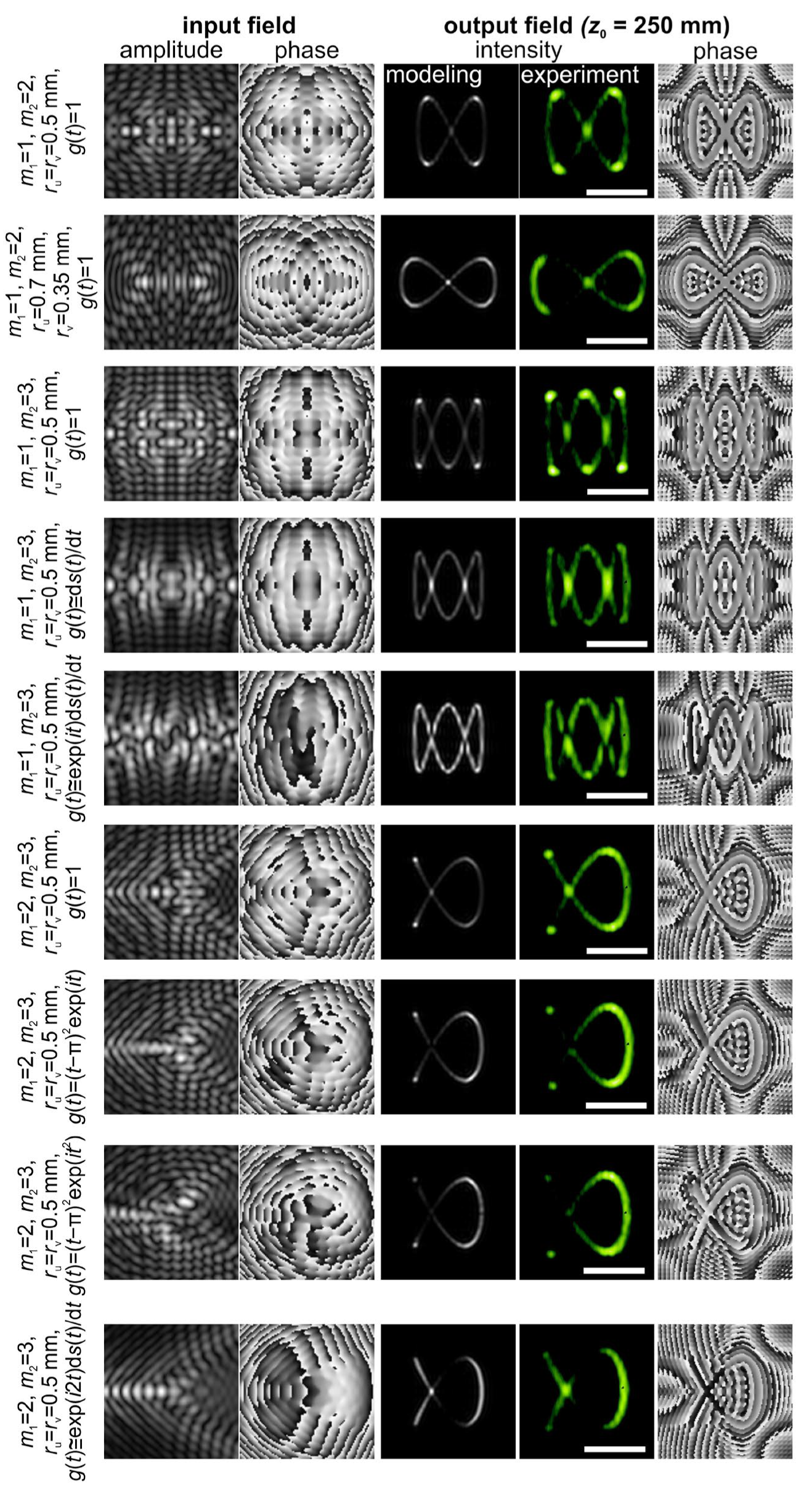
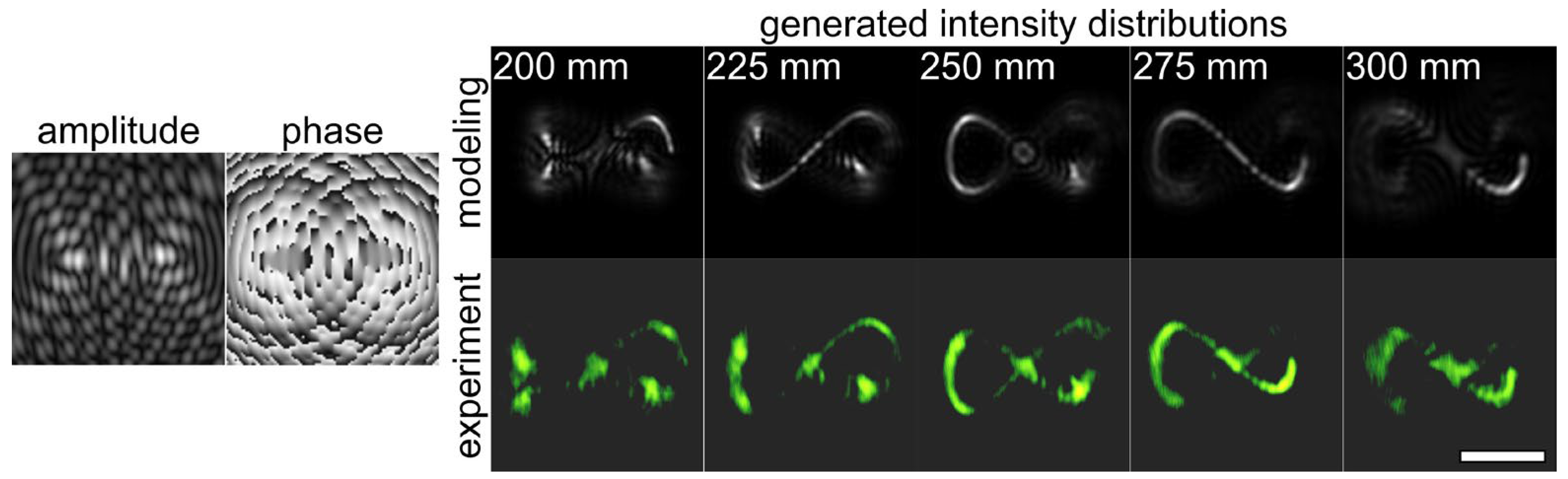
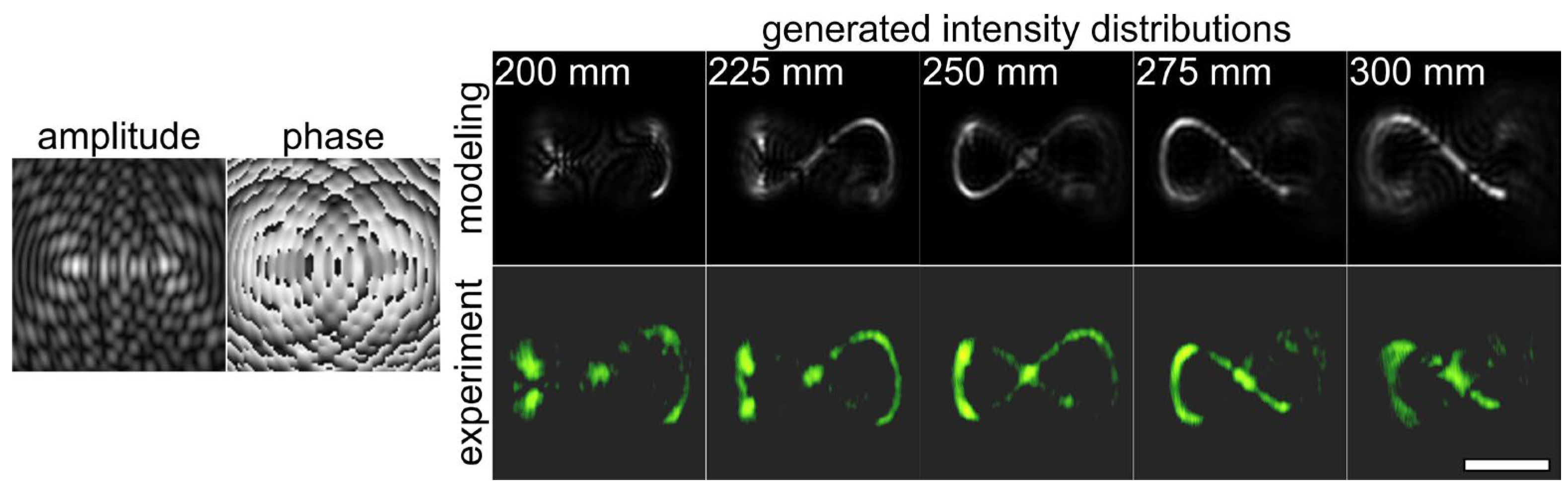
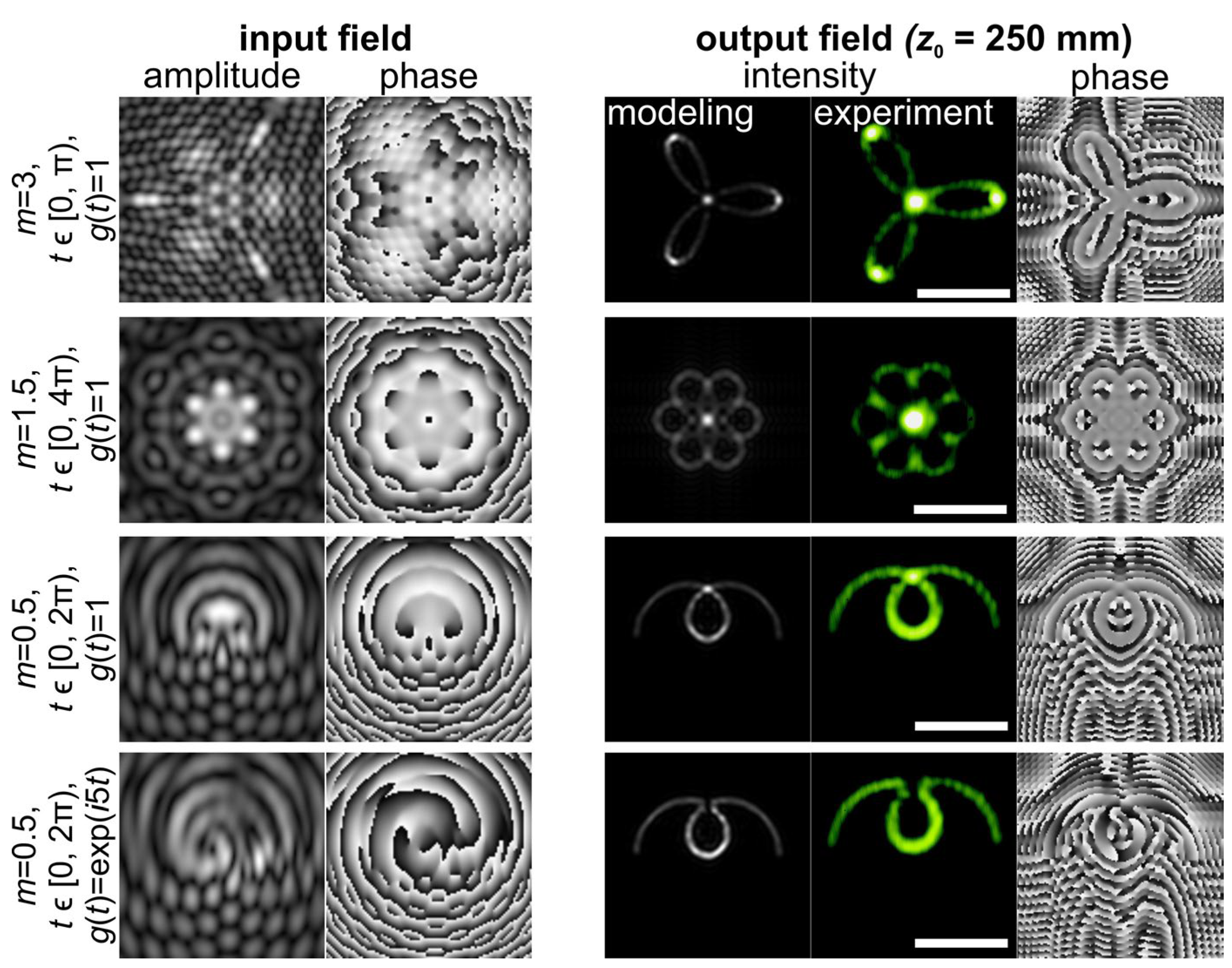
3.3. Lissajous Figures
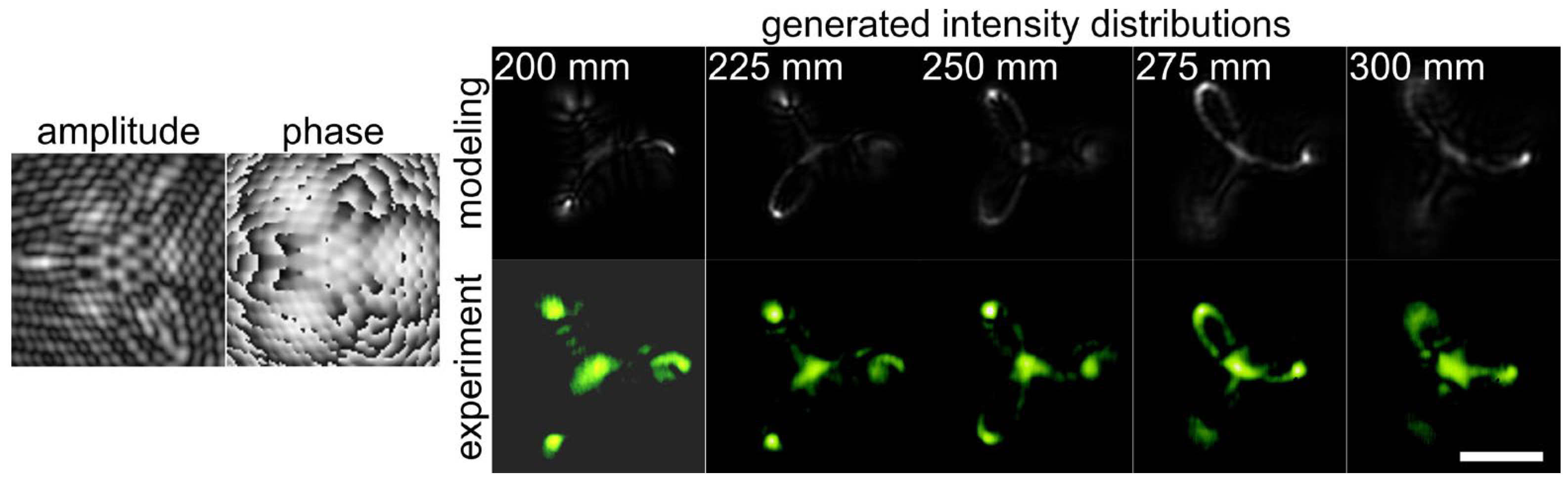
3.4. Rose Curves
4. Discussion
5. Conclusions
Author Contributions
Funding
Institutional Review Board Statement
Informed Consent Statement
Data Availability Statement
Conflicts of Interest
References
- Kritzinger, A.; Forbes, A.; Forbes, P.B.C. Optical Trapping and Fluorescence Control with Vectorial Structured Light. Sci. Rep. 2022, 12, 17690. [Google Scholar] [CrossRef] [PubMed]
- Otte, E.; Denz, C. Optical Trapping Gets Structure: Structured Light for Advanced Optical Manipulation. Appl. Phys. Rev. 2020, 7, 041308. [Google Scholar] [CrossRef]
- Zhou, L.M.; Shi, Y.; Zhu, X.; Hu, G.; Cao, G.; Hu, J.; Qiu, C.W. Recent Progress on Optical Micro/Nanomanipulations: Structured Forces, Structured Particles, and Synergetic Applications. ACS Nano 2022, 16, 13264–13278. [Google Scholar] [CrossRef] [PubMed]
- Singh, B.K.; Nagar, H.; Roichman, Y.; Arie, A. Particle Manipulation Beyond the Diffraction Limit Using Structured Super-Oscillating Light Beams. Light Sci. Appl. 2017, 6, e17050. [Google Scholar] [CrossRef]
- Yang, Y.; Ren, Y.X.; Chen, M.; Arita, Y.; Rosales-Guzmán, C. Optical Trapping with Structured Light: A Review. Adv. Photon. 2021, 3, 034001. [Google Scholar]
- Flamm, D.; Grossmann, D.G.; Sailer, M.; Kaiser, M.; Zimmermann, F.; Chen, K.; Jenne, M.; Kleiner, J.; Hellstern, J.; Tillkorn, C.; et al. Structured Light for Ultrafast Laser Micro-and Nanoprocessing. Opt. Eng. 2021, 60, 025105. [Google Scholar] [CrossRef]
- Malinauskas, M.; Žukauskas, A.; Hasegawa, S.; Hayasaki, Y.; Mizeikis, V.; Buividas, R.; Juodkazis, S. Ultrafast Laser Processing of Materials: From Science to Industry. Light Sci. Appl. 2016, 5, e16133. [Google Scholar] [CrossRef]
- Porfirev, A.; Khonina, S.; Kuchmizhak, A. Light–Matter Interaction Empowered by Orbital Angular Momentum: Control of Matter at the Micro-and Nanoscale. Prog. Quantum. Electron. 2023, 88, 100459. [Google Scholar] [CrossRef]
- Jesacher, A.; Maurer, C.; Schwaighofer, A.; Bernet, S.; Ritsch-Marte, M. Full Phase and Amplitude Control of Holographic Optical Tweezers with High Efficiency. Opt. Express 2008, 16, 4479–4486. [Google Scholar] [CrossRef]
- Syubaev, S.; Zhizhchenko, A.; Kuchmizhak, A.; Porfirev, A.; Pustovalov, E.; Vitrik, O.; Kulchin, Y.; Khonina, S.; Kudryashov, S. Direct Laser Printing of Chiral Plasmonic Nanojets by Vortex Beams. Opt. Express 2017, 25, 10214–10223. [Google Scholar] [CrossRef]
- Syubaev, S.; Porfirev, A.; Zhizhchenko, A.; Vitrik, O.; Kudryashov, S.; Fomchenkov, S.; Khonina, S.; Kuchmizhak, A. Zero-Orbital-Angular-Momentum Laser Printing of Chiral Nanoneedles. Opt. Lett. 2017, 42, 5022–5025. [Google Scholar] [CrossRef] [PubMed]
- Ambrosio, A.; Marrucci, L.; Borbone, F.; Roviello, A.; Maddalena, P. Light-Induced Spiral Mass Transport in Azo-Polymer Films under Vortex-Beam Illumination. Nat. Commun. 2013, 3, 989. [Google Scholar] [CrossRef]
- Takahashi, F.; Miyamoto, K.; Hidai, H.; Yamane, K.; Morita, R.; Omatsu, T. Picosecond Optical Vortex Pulse Illumination Forms a Monocrystalline Silicon Needle. Sci. Rep. 2016, 6, 21738. [Google Scholar] [CrossRef] [PubMed]
- Dholakia, K.; Lee, W.M. Optical Trapping Takes Shape: The Use of Structured Light Fields. Adv. At. Mol. Opt. Phys. 2008, 56, 261–337. [Google Scholar]
- Rodrigo, J.A.; Alieva, T. Freestyle 3D Laser Traps: Tools for Studying Light-Driven Particle Dynamics and Beyond. Optica 2015, 2, 812–815. [Google Scholar] [CrossRef]
- Ni, J.; Wang, C.; Zhang, C.; Hu, Y.; Yang, L.; Lao, Z.; Xu, B.; Li, J.; Wu, D.; Chu, J. Three-Dimensional Chiral Microstructures Fabricated by Structured Optical Vortices in Isotropic Material. Light Sci. Appl. 2017, 6, e17011. [Google Scholar] [CrossRef]
- Huang, T.D.; Lu, T.H. Controlling an Optical Vortex Array from a Vortex Phase Plate, Mode Converter, and Spatial Light Modulator. Opt. Lett. 2019, 44, 3917–3920. [Google Scholar] [CrossRef]
- Shen, S.; Yang, Z.; Li, X.; Zhang, S. Periodic Propagation of Complex-Valued Hyperbolic-Cosine-Gaussian Solitons and Breathers with Complicated Light Field Structure in Strongly Nonlocal Nonlinear Media. Commun. Nonlinear Sci. Numer. Simul. 2021, 103, 106005. [Google Scholar] [CrossRef]
- Xu, J.; Liu, Z.; Pan, K.; Zhao, D. Asymmetric Rotating Array Beams with Free Movement and Revolution. Chin. Opt. Lett. 2022, 20, 022602. [Google Scholar] [CrossRef]
- Song, L.-M.; Yang, Z.-J.; Li, X.-L.; Zhang, S.-M. Coherent Superposition Propagation of Laguerre–Gaussian and Hermite–Gaussian Solitons. Appl. Math. Lett. 2020, 102, 106114. [Google Scholar] [CrossRef]
- Efremidis, N.K.; Chen, Z.; Segev, M.; Christodoulides, D.N. Airy Beams and Accelerating Waves: An Overview of Recent Advances. Optica 2019, 6, 686–701. [Google Scholar] [CrossRef]
- Lee, G.-Y.; Yoon, G.; Lee, S.-Y.; Yun, H.; Cho, J.; Lee, K.; Kim, H.; Rho, J.; Lee, D. Complete Amplitude and Phase Control of Light Using Broadband Holographic Metasurfaces. Nanoscale 2018, 10, 4237–4245. [Google Scholar] [CrossRef] [PubMed]
- Chen, Y.; Wang, T.; Ren, Y.; Fang, Z.; Ding, G.; He, L.; Lu, R.; Huang, K. Generalized Perfect Optical Vortices Along Arbitrary Trajectories. J. Phys. D Appl. Phys. 2021, 54, 214001. [Google Scholar] [CrossRef]
- Tang, X.; Nan, F.; Yan, Z. Rapidly and Accurately Shaping the Intensity and Phase of Light for Optical Nano-Manipulation. Nanoscale Adv. 2020, 2, 2540–2547. [Google Scholar] [CrossRef] [PubMed]
- Rodrigo, J.A.; Alieva, T. Polymorphic Beams and Nature Inspired Circuits for Optical Current. Sci. Rep. 2016, 6, 35341. [Google Scholar] [CrossRef] [PubMed]
- Rodrigo, J.A.; Alieva, T.; Abramochkin, E.; Castro, I. Shaping of Light Beams Along Curves in Three Dimensions. Opt. Express 2013, 21, 20544–20555. [Google Scholar] [CrossRef] [PubMed]
- Zhao, J.; Chremmos, I.D.; Song, D.; Christodoulides, D.N.; Efremidis, N.K.; Chen, Z. Curved Singular Beams for Three-Dimensional Particle Manipulation. Sci. Rep. 2015, 5, 12086. [Google Scholar] [CrossRef] [PubMed]
- Yan, S.; Yu, X.; Li, M.; Yao, D. Curved Optical Tubes in a 4Pi Focusing System. Opt. Express 2015, 23, 22890–22897. [Google Scholar] [CrossRef] [PubMed]
- Khonina, S.N.; Koltyar, V.V.; Soifer, V.A. Techniques for Encoding Composite Diffractive Optical Elements. Proc. SPIE 2003, 5036, 493–498. [Google Scholar]
- Doskolovich, L.L.; Dmitriev, A.Y.; Bezus, E.A.; Moiseev, M.A. Analytical Design of Freeform Optical Elements Generating an Arbitrary-Shape Curve. Appl. Opt. 2013, 52, 2521–2526. [Google Scholar] [CrossRef]
- Vijayakumar, A.; Bhattacharya, S. Design, Fabrication and Evaluation of Diffractive Optical Elements for Generation of Focused Ring Patterns. Proc. SPIE 2015, 9449, 944902. [Google Scholar]
- Khorin, P.A.; Porfirev, A.P.; Khonina, S.N. Composite Diffraction-Free Beam Formation Based on Iteratively Calculated Primitives. Micromachines 2023, 14, 989. [Google Scholar] [CrossRef] [PubMed]
- Wang, Z.; Zhang, N.; Yuan, X.-C. High-Volume Optical Vortex Multiplexing and Demultiplexing for Free-Space Optical Communication. Opt. Express 2011, 19, 482–492. [Google Scholar] [CrossRef] [PubMed]
- Kazanskiy, N.L.; Khonina, S.N.; Karpeev, S.V.; Porfirev, A.P. Diffractive Optical Elements for Multiplexing Structured Laser Beams. Quantum Electron. 2020, 50, 629–635. [Google Scholar] [CrossRef]
- Ortiz-Ambriz, A.; Lopez-Aguayo, S.; Kartashov, Y.V.; Vysloukh, V.A.; Petrov, D.; Garcia-Gracia, H.; Gutiérrez-Vega, J.C.; Torner, L. Generation of Arbitrary Complex Quasi-Non-Diffracting Optical Patterns. Opt. Express 2013, 21, 22221–22231. [Google Scholar] [CrossRef]
- Bekshaev, A.Y.; Soskin, M.S. Transverse Energy Flows in Vectorial Fields of Paraxial Beams with Singularities. Opt. Commun. 2007, 271, 332–348. [Google Scholar] [CrossRef]
- Bekshaev, A.Y. Internal Energy Flows and Instantaneous Field of a Monochromatic Paraxial Light Beam. Appl. Opt. 2012, 51, C13–C16. [Google Scholar] [CrossRef]
- Goorden, A.; Bertolotti, J.; Mosk, A.P. Superpixel-Based Spatial Amplitude and Phase Modulation Using a Digital Micromirror Device. Opt. Express 2014, 22, 17999–18009. [Google Scholar] [CrossRef]
- Kovalev, A.A.; Kotlyar, V.V.; Porfirev, A.P. Generation of Half-Pearcey Laser Beams by a Spatial Light Modulator. Comput. Opt. 2014, 38, 658–662. [Google Scholar] [CrossRef]
- Kessler, D.A.; Freund, I. Lissajous singularities. Opt. Lett. 2003, 28, 111–113. [Google Scholar] [CrossRef]
- Alonzo, C.A.; Rodrigo, P.J.; Glückstad, J. Helico-Conical Optical Beams: A Product of Helical and Conical Phase Fronts. Opt. Express 2005, 13, 1749–1760. [Google Scholar] [CrossRef] [PubMed]
- Cheng, S.B.; Xia, T.; Liu, M.S.; Jin, Y.Y.; Zhang, G.; Tao, S.H. Power-Exponent Helico-Conical Optical Beams. Opt. Laser Technol. 2019, 117, 288–292. [Google Scholar] [CrossRef]
- Khonina, S.N.; Ustinov, A.V.; Logachev, V.I.; Porfirev, A.P. Properties of Vortex Light Fields Generated by Generalized Spiral Phase Plates. Phys. Rev. A 2020, 101, 043829. [Google Scholar] [CrossRef]
- Xia, T.; Tao, S.H.; Cheng, S.B. A Spiral-Like Curve with an Adjustable Opening Generated by a Modified Helico-Conical Beam. Opt. Commun. 2020, 458, 124824. [Google Scholar] [CrossRef]
- Khonina, S.N.; Ustinov, A.V.; Porfirev, A.P. Diatom Optical Element: A Quantized Version of the Generalized Spiral Lens. Opt. Lett. 2022, 47, 3988–3991. [Google Scholar] [CrossRef]


Disclaimer/Publisher’s Note: The statements, opinions and data contained in all publications are solely those of the individual author(s) and contributor(s) and not of MDPI and/or the editor(s). MDPI and/or the editor(s) disclaim responsibility for any injury to people or property resulting from any ideas, methods, instructions or products referred to in the content. |
© 2023 by the authors. Licensee MDPI, Basel, Switzerland. This article is an open access article distributed under the terms and conditions of the Creative Commons Attribution (CC BY) license (https://creativecommons.org/licenses/by/4.0/).
Share and Cite
Khonina, S.N.; Porfirev, A.P.; Volotovskiy, S.G.; Ustinov, A.V.; Karpeev, S.V. Simple Method of Light Field Calculation for Shaping of 3D Light Curves. Photonics 2023, 10, 941. https://doi.org/10.3390/photonics10080941
Khonina SN, Porfirev AP, Volotovskiy SG, Ustinov AV, Karpeev SV. Simple Method of Light Field Calculation for Shaping of 3D Light Curves. Photonics. 2023; 10(8):941. https://doi.org/10.3390/photonics10080941
Chicago/Turabian StyleKhonina, Svetlana N., Alexey P. Porfirev, Sergey G. Volotovskiy, Andrey V. Ustinov, and Sergey V. Karpeev. 2023. "Simple Method of Light Field Calculation for Shaping of 3D Light Curves" Photonics 10, no. 8: 941. https://doi.org/10.3390/photonics10080941