1. Introduction
Metallic nanoparticles are currently being intensively studied both in terms of describing their interaction with electromagnetic radiation and for utilizing their unique properties. Their application as plasmonic nanostructured materials can find use in various fields, such as sensors utilizing the effect of phosphorescence [
1], extraordinary optical transmission (EOT) [
2], photothermal applications [
3], Raman spectroscopy (SERS) [
4,
5], designs of highly sensitive gas sensors [
6,
7,
8,
9], unique anti-reflective coatings to enhance the efficiency of solar cells [
10], integrated optical or quantum signal processing [
11], battery research [
12,
13], biomedical applications [
4,
14,
15], and even in designing metamaterials with unique properties such as negative refractive index [
16], among others.
The existing research and development of new applications in the aforementioned directions, necessarily relies on adequately precise calculations. At the current level of knowledge, approximate solutions in the form of quasistatic models appear insufficient [
17,
18], even though in the early days of plasmonics, these theories provided many satisfactory explanations [
19]. A fundamental breakthrough for the entire field of plasmonics was represented by Mie’s theory [
20], which accurately determined the position and value of resonant extinction maxima and associated quantities characterizing the behavior of spherical particles interacting with incident electromagnetic waves.
The demand for accuracy in description, and thus the relevance of simulations derived from them, increases in parallel with the growing technological capabilities of preparations of nanostructures and nanostructured surfaces [
21,
22,
23]. As an example, sensor applications based on SERS technology can be mentioned, where the sensitivity of the sensor relies on the amplification of the field at the specifically designed site where the binding of the detected molecule is intended to occur.
Just as the quasistatic theory has proven to be inadequate, the classical solutions of Maxwell’s equations now also appear unsatisfactory, particularly when a high precision of results is required to simulate the interaction of plasmonic nanostructures with electromagnetic waves. Based on numerous experiments, it is becoming evident that standard simulations, in some cases, significantly overestimate the intensity of the electromagnetic field in the vicinity of sharp edges and interfaces of nanostructures [
24]. In the case of nanostructures with characteristic dimensions on the order of a few nanometers, as mentioned above, the classical theory also inaccurately determines the position of resonant maxima for characteristic quantities.
These shortcomings can become a significant problem in practice. A clear example can be found in sensor applications, where in addition to accurately determining the resonant frequency, the intensity of the electric field in specific detection locations of the sensor also plays a significant role. The mentioned requirements for high calculation accuracy have given rise to the need to incorporate nonlocal response.
In contrast to the classical description (Maxwell’s equations and Ampere’s law), the nonlocal theory assumes a more complex relationship between current density and electric field evolution than a simple proportional relationship. The most widely used nonlocal model in the field of plasmonics has become the so-called standard hydrodynamic model (HDM) [
25]. However, there are also alternative nonlocal models [
26,
27].
Using the HDM, Mie theory has already been generalized [
28,
29], and several other analytical solutions have been found for metallic interfaces [
30], such as the generalized Fresnel equations [
31,
32]. For the structure of an infinitely long cylinder, the need for finding an accurate solution has been demonstrated, as the so-called curl-free approximation exhibits significant numerical drawbacks in the form of spurious resonances below the plasma frequency [
33].
While the standard HDM has become a successful mathematical tool for predicting various phenomena, such as the blue shift of the main extinction maximum in gold and silver spherical nanoparticles with diameters smaller than 10 nm, theoretical research in this field continues with the aim of achieving the most accurate description. Recently, a modification of HDM called GNOR (general nonlocal optical response) has been proposed [
34,
35] which incorporates the diffusion of the electron gas. The influence of Landau (Kreibig) damping, which is inversely proportional to the nanoparticle size [
36,
37,
38], is also being discussed. Simultaneously, efforts are being made to find solutions for a more accurate nonlinearized form of HDM [
39,
40], and the question of viscosive damping of the electron gas is gaining prominence [
41,
42,
43,
44]. The hydrodynamic model itself is based on the concept of a jellium model which can be interpreted as the electron fluid moving with respect to a positively charged background of metal ions. From this perspective, the question directly arises of how much of the overall material response of a metal belongs to the electron fluid itself and how much to the ion background. The standard HDM, for example, does not consider the influence of energy transitions of electrons within the conduction band, and thus this response is implicitly attributed from a mathematical perspective to the ion background of a metal. From the description of fluid dynamics, there is also a well-known connection between diffusion and viscosive damping, which suggests incorporating the influence of diffusion in an alternative way, different from the GNOR modification. These aforementioned insights are, in our opinion, a relevant stimulus for considering further possible modifications of the hydrodynamic model, which is also the main goal of our article.
The contributions of our article are thus numerous. Among other things, we provide a relatively detailed mathematical procedure for solving HDM in the case of the interaction of a metallic spherical particle with a planar wave. We also compare selected calculations between the classical (Mie) and nonlocal HD models. However, the main contribution lies in presenting a possible approach for further generalizing the standard HDM through the modification of the existing GNOR-HDM by incorporating viscosive damping and considering the general form of the Drude–Lorentz term. Furthermore, in analogy with the previous approach, we compare the computations obtained by solving each variant of the HDM.
The remaining sections of the article are organized as follows: in the second section of the article, we briefly recapitulate the procedure of solving the problem of the interaction between a plane wave and a spherical metal nanoparticle within the framework of the HD model, and subsequently present important new results in the form of an explicit expression for the field expansion coefficients; in the third section, the effective extinction cross sections of gold and silver particles determined according to the classical Mie theory and the standard HD model are compared. Additionally, the influence of Kreibig damping on the behavior of the mentioned quantities is briefly analyzed; the fourth section is dedicated to the generalization of the GNOR-HDM, so that the new model incorporates viscosive damping of the electron gas and the general Drude–Lorentz term. Furthermore, the procedure for the possible solution of our modified GNOR-HDM is discussed; the final fifth section of the article is focused on comparing the results of individual variants of HD models, with the emphasis on comparing the calculations of selected quantities using the standard HD model and our generalized GNOR-HDM, also referred to as the HD model with viscosive damping; finally, the paper is concluded with the conclusions together with possible future activities.
2. Review of the Standard Hydrodynamic Model and Calculation Procedure
In this section, we review the standard hydrodynamic model calculation procedure [
29], and subsequently also show our implementation of the technique (
Section 3), which will be later used for the generalized hydrodynamic model (
Section 4). From a mathematic point of view, the HD model and its modifications represents a system of two linear differential equations for the vector functions of the electric field
and the induced current density
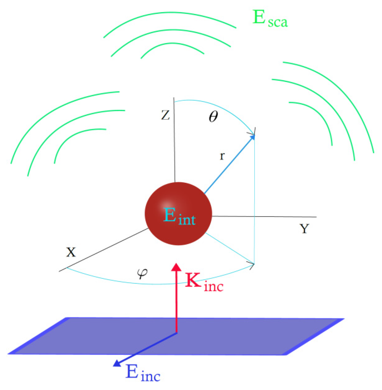
. In this article, we will use simplified notation for vector functions
,
, where
is the angular frequency and
,
, and
are the spherical coordinates (see
Figure 1).
In the traditional HDM, the electrical field and the current density are given by the solutions of the wave equation and the hydrodynamic equation-of-motion [
38]. We will concentrate here on the specific spherical geometry of a nanoparticle, although some parts of the calculation are more general (primarily the determination of the nonlocal wave number). Clearly, derived expansion coefficients of the fields are generally dependent on the particle shape and analytically can be determined only for a spherical geometry considered here.
The basic HD model can be formulated with Equations (1) and (2) as follows:
Here, the constants , and represent vacuum permittivity, vacuum permeability, and the speed of light, respectively. Next, quantities of the HD model and indicate the permittivity of electron gas and the total permittivity of a metal, respectively.
The next assumption is concerned with the expression for the permittivity of an electron gas. The HDM modification unfortunately provides no clue which particular form should represent the electron gas permittivity. Clearly, one possibility is to use the expression often formulated in the literature; for example in [
45,
46]. This expression for the electron gas permittivity is, in fact, the Drude–Lorentz relation for the permittivity, and can be stated as follows:
Here, the difference
has the meaning of permittivity of the ionic background of the metal. Other parameters of the HD model are the plasma angular frequency
, the attenuation constant
, and the nonlocal constant
, where
is the Fermi velocity. At this point, it is appropriate to provide specific values for the parameters. According to [
38], for gold, the values are
,
and
, in the case of silver, the values are
,
and
. The mentioned values of parameters are used in the analysis of selected quantities in the third and fifth part of this article.
For solving this system of equations, at first it is necessary to determine both longitudinal and transversal wave numbers, as applied, e.g., in [
29]. We note that while the longitudinal wave number belongs to the electric field with the vector of electric intensity oscillating in the direction of the wave vector of the field, the transversal wave number belongs to the field which oscillates perpendicularly with respect to the direction of propagation. Following [
29], the transversal and longitudinal field components can be described as
and
, respectively, where
is the transversal electric field,
is some vector function,
is the longitudinal electric field and
some scalar function. Although these assumptions are not absolutely general, they are typically used (as in Equation (1)) and allow us to obtain the analytical results, as required. It should be also noted that there exists an alternative procedure based on the mathematical theory of generalized functions [
2], but this approach brings another difficulty connected with the fulfillment of the boundary conditions and thus is not very practical. A reader can find a classification of HD models from the perspective of such a generalized function (including also the derivation of Green functions) in [
47]. Returning to our approach, for the spherical geometry considered,
is therefore necessarily a spherical vector function and the
function satisfies the scalar wave equation. The fields
and
, hence, satisfy the following Equations (4) and (5), respectively; this follows from the definition of vector spherical harmonics.
Further, these relations (4) and (5) will be substituted into Equations (1) and (2), to obtain the following equations
These two equations can be further converted to describe the longitudinal and transversal fields separately. This will enable assuming the fields can be described by scalar functions and hence the mathematical operators of rotation and gradient can be applied to them, providing for the longitudinal case
and similarly, for the transversal field and transversal wave number
This will further allow expressing the longitudinal wave number from Equations (8) and (9), and correspondingly, the transversal wave number, from Equations (10) and (11), as
Unfortunately, if we assume that
is zero, as it follows from standard Maxwell equations, then nonphysical results appear, specifically, the extinction cross section will follow wrong functional dependence and the extinction maxima will not follow correct spectral position for bigger particles, in accordance with the Mie theory. Here, we will track the calculation method, introduced in [
29], to obtain the correct results. The idea of this technique is based on expressing the unknown permittivity of an electron gas
as
(see Equations (3) and (12)). Applying this, the transversal wave number follows the predictions for the electric and magnetic fields from the Mie theory [
48]. The HD model, however, as compared to the standard Mie theory, also considers the longitudinal wave number (which often has a significantly larger value). Clearly, from the wave number formulas, one can further proceed with the calculations of the scattered field around a particle and the induced field in a particle (i.e., the absorbed field). First, we must specify the proper boundary conditions. Although Maxwell boundary conditions allow discontinuity of the tangential magnetic field component, the Mie theory assumes their continuity. The same boundary conditions are used in the case of solving HDM in [
29]. Second, the tangential electric field is naturally continuous on the boundary of a particle. Finally, the last boundary condition determines the zero normal component of the electric current density on the particle boundary. Overall, following the expansion of the fields in the spherical coordinates
, we obtain five boundary conditions on the particle boundary
Here, , and , are the components of the total electric and magnetic field inside a particle, in the directions of spherical coordinates and , respectively. Similarly, , and , are the components of the scattered fields, and , and , represent the incident fields. All fields are considered on the surface of a particle. Before starting the determination of expansion coefficients of the fields, let us make some remarks. We will follow the procedure of decomposing the transversal fields into series of vector spherical wave functions M and N of both even (index e) and odd (index o) components which we will denote as , ,,,,,,. Here, the index n belongs to the radial part whereas the index m represents the azimuthal part of the wave function, respectively.
In order to describe the longitudinal fields, it is necessary to find the solution of Equation (5) in spherical coordinates. We will thus define the scalar even and odd functions and . It is also convenient to distinguish the mentioned functions according to the wave number in the argument of their radial functions, therefore we add the given wave number as the superscript of the respective functions. The index n takes values from 1,2…∞, the index m should be restricted only to the values −1 or 1 because we consider the case of a single spherical particle and an incident plane wave. Clearly, in the case of a Gaussian beam (or an evanescent wave), this symmetry is broken. The vector functions with no upper index are expressed with radial spherical Bessel functions , vector functions with index h include a spherical Hankel function of the first type . Index o denotes the odd function and index e denotes the even function .
The mathematical form of the vector spherical harmonics in the spherical coordinates
,
θ, and
φ are well known, and can be found, for example in [
20] or [
49]. The explicit expression of the gradient of the
and
functions necessary for the decomposition of the longitudinal fields is thus as follows:
Using the vector harmonics
M and
N and the gradients of the scalar functions mentioned above, it is possible to decompose the fields. For the selected index
m and
n, the following relations can be found:
Relations (19) and (20) hold for the incident plane wave, see
Figure 1, and its electric and magnetic components, respectively. The electric and magnetic fields and the induced current density inside the particle can be determined by Equations (21)–(23). Similar to the incident field around the particle, relations for the scattered field can be established in the form of Equation (24) for the electric field and (25) for the magnetic field.
The individual wave numbers are marked as follows:
is the (vacuum) wave number of the incident and scattered field,
and
are the wave numbers of the transversal and longitudinal fields inside the nanoparticle. Parameters S and T take the following form
,
. To obtain the total fields
and current density
, it is necessary to sum the components in Equations (19)–(25), over all
n and
m. Before summation, one must determine ten unknown coefficients,
by substituting the components from Equations (19)–(25) into Equations (14)–(16). In our situation of the nonlocal case, the gradients in Equations (17) and (18) will be applicable. Next, we can proceed with solving five boundary conditions using the finding that the expansion coefficients
are, in fact, zero. That is implied by the fact that we have only five linear equations for the ten unknowns. It is thus possible to determine the expansion coefficients in the form shown below. Here, it is convenient to define the following effective labelling:
,
,
,
, and similarly for other indices. The expansion coefficients
,
,
,
, after some algebraic manipulation, take the following form:
In order to facilitate the reader’s possible work when deriving these expansion coefficients for the fields, we present here their explicit expressions. Now, from the knowledge of the
and
coefficients, it is clearly possible to evaluate the effective cross-section of extinction:
The expansion coefficients , ,, are also necessary for calculation of induced current density in a particle, electric and magnetic fields in the surroundings and within the volume of a particle. The coefficients have a general form for the spherical particle, therefore parametric modifications of the HD model would change only the formulas for the wave numbers and electron gas permittivities.
One possible modification of the HD model is the so-called general nonlocal optical response (GNOR) theory [
34,
38]. This theory should unify quantum-pressure convection effects and induced charge-diffusion kinetics. GNOR also describes size-dependent damping and corresponding frequency shifts. By considering the diffusion effect within the GNOR model, the nonlocal constant is modified as follows:
, where
is the diffusion constant that can be estimated using the relation
. The diffusion effect modifies the nonlocal constant which manifests as a change in the longitudinal wave number. This effect could be easily added to our model, too. Another possible modification concerns the correction of the damping constant value with respect to the particle size. Experimental measurements of extinction spectra of small plasmonic particles using EELS (electron energy loss spectroscopy) have revealed broadening and shifts of the resonance peaks which can be explained by the size-dependent dependence of the damping constant. Phenomenologically, as proposed by Kreibig, this phenomenon can be described by a correction to the damping constant, where
. From the theoretical explanation of this phenomenon found by Landau [
37], it follows that the enhanced damping is a result of the direct excitation of electron-hole pairs in the metal within the region of highly confined surface plasmon field. For a spherical metal particle, one can deduce [
34] an estimate
, this estimation was used in our model. The effect of this attenuation on the spectral behavior of the extinction will be shown in the next section.
4. Nonlocal Hydrodynamic Model with Viscosive Damping and Generalized Drude–Lorentz Term
The standard HDM, analyzed in the previous section, is based on the perception of an electron gas as a charged continuum which can be described, in a certain approximation with a model, relying on the equations of motion of a fluid flow. Recently, an extension of the HDM has been proposed that includes the diffusion of an electron gas; a phenomenon occurring regularly in liquids and gases. Within the physics of fluids, the Stokes–Navier equations play a crucial role, which, among other issues, establishes a close connection between diffusion and viscosive damping. Therefore, it is natural to generalize the standard HDM by introducing viscosive damping of the electron fluid. Starting from the derivation of HDM in [
25] and the Stokes–Navier equations for the case of convective form [
50], it is straightforward to arrive at the initial Equation (32), which can be further modified to find the generalized variant of HDM.
The left-hand side of Equation (32) represents the total derivative of the velocity vector
v of the electron fluid with respect to time. The first term on the right-hand side represents the Lorentz force acting on an individual volume element of the electron fluid. The second term is the standard damping term, the third term is the standard nonlocal expression, and the last two terms of the equation involve viscosive damping. The individual parameters of the model are as follows:
B is the magnetic field,
is the mass density of the electron fluid,
is the charge of the electron,
is the charge density,
is the same nonlocal constant as in the standard HDM, and terms
and
represent the relevant damping terms of viscosive attenuation in the convective form of the Navier–Stokes equation.
To proceed further, it is first convenient to assume the behavior of the electron gas density in the form:
, where
is a constant equilibrium density and
is a linear deviation. Subsequently, it is possible to linearize the Equation (32), which leads to neglecting the influence of the magnetic field and introducing an approximate expression for the current density, charge density and mass density as:
,
, and
, where
is the electron mass. If we multiply Equation (32) by the term
and perform the mentioned linearization, we obtain:
If we introduce a new damping parameter,
, which is analogous to kinematic viscosity in the classical approach, and further, according to the common definition, the plasma frequency
, then by straightforward adjustments of Equation (33), we obtain a modified novel version of the first equation of the standard HDM as follows:
Now the question arises whether it is possible to further generalize Equation (34). Since the HDM can be considered as a more sophisticated version of the Drude model for the electron dispersion in a metal, it is worth considering a similar modification approach as in the case of the actual Drude model. As it is well known, the original Drude model of the permittivity of a metal can be modified by the additional Lorentzian terms, resulting in the Drude–Lorentz model [
51,
52], to account for intraband (within the conduction band) and interband (between bands) electron energy transitions. By a simple analysis of the first equation of the HDM, i.e., the current Equation (34), by substituting the transverse fields, it can be determined that precisely the term
is crucial for the Drude-type response of the permittivity
of a free electron gas. Let us assume a generalization:
, where
is an as-yet undetermined function. For better clarity, let us denote
and introduce an HDM with viscosive damping and a generalized Drude–Lorentz term in the following form:
The generalized HDM defined by Equations (35) and (36) includes the three unknown parameters
,
,
for which it will be necessary to establish the three conditions. The term
has a similar meaning as
in the case of classical HDM, representing the permittivity of the electron gas, but it is generally different from
. The total permittivity
of the metal is the same as in the classical HDM and is determined by tabulated values [
53]. All these three parameters are clearly frequency dependent, however, for the sake of clarity in the mathematical notation, it will not be shown here.
Finding a solution for the generalized HDM is possible in a similar way to the classical HDM. From Equation (36), it is possible to express the relationship for current density
and substitute it into Equation (35). In this way, an equation for the total electric field
only is obtained, which can be solved separately for its transverse and longitudinal components. In the case of a transverse field, it is advantageous to use the relationships between vector spherical harmonics
and operator identities:
,
, valid for any vector function
. In the case of a longitudinal field, it is beneficial to use the identities
and
. Based on the mentioned procedure, the relationships for the transversal and longitudinal wave numbers can be obtained in the following form:
Equations (37) and (38) serve as a starting point for finding the additional relationships for the parameters
,
, and
. The classical HDM already includes a closely unspecified parameter
. However, to ensure that the HDM solution is not too far from the experimentally measured values, a condition
has been introduced for the transverse wave number [
29] which is widely utilized, and which will be also applied here. Considering that the standard solution of Equation (37) as a quadratic equation would provide only one condition, it seems reasonable to proceed by evaluating the brackets in (37), which allows us to obtain a pair of additional expressions without the need for the introduction of ad hoc parameters. One possibility is to set the second term in Equation (37) equal to
and the third term equal to zero. However, it can be easily verified that such a solution implies a zero value for the longitudinal wave number and therefore the absence of the nonlocal response. One option is to set the second term in Equation (37) equal to
and the third term equal to zero. However, such a solution implies a zero value for the longitudinal wave number, and therefore the absence of a nonlocal response. Therefore, as a solution, it is suggested to set the first bracket in Equation (37) to zero and assign the value of
to the last term in Equation (37). From Equation (37), we can easily obtain two conditions in the following form:
To establish the final condition, it is possible to start from the following consideration. Let us assume that the diffusion phenomenon is well phenomenologically described by the GNOR modification [
34] of the HDM, although the magnitude of the diffusion constant
may still be the subject of investigation [
38]. Thanks to the fact that the fourth term in the right-hand side of Equation (32) is responsible for the diffusion according to the classical description of fluid dynamics, this diffusion is indeed included in Equation (32). From the comparison of the GNOR model with the classical HD, it follows that diffusion manifests only in the change in the nonlocal parameter as:
. Under the assumption that diffusion is the main accompanying phenomenon caused by viscosive damping, it can be presumed that such viscosive damping will manifest in a similar way, primarily through a certain change in the nonlocal constant
. Based on the mentioned considerations and Equation (38), the third condition can be written in the following form:
From the given conditions (39)–(41), the relationships for the parameters
and
can be derived. Specifically, from Equations (39) and (41), it is straightforward to obtain the following relationship for
as:
Subsequently, from Equations (40)–(42), the relationship for
can be derived in the following form:
From the above Equations (41)–(43), it is finally possible to determine the longitudinal wave number defined by (38). As mentioned before, for the transverse wave number, the relationship
holds. The value of the diffusion constant can be approximated as
according to [
38,
53] which we have also used in our calculations. It remains to be mentioned that the expansion coefficients of the fields, including the substitution relations denoted by
and
, given in the second section, can be still used in the same form, but with a logical replacement of
,
, and
by
,
, and
. For the calculation of extinction, the same approach as in the case of the classical HDM, is clearly now applicable as well. The Formulas (26) to (30), together with Equation (31), can be used, with the difference that the longitudinal wave number is now determined with the new corresponding relation, i.e., according to Equation (38).
5. Results of HDM with Generalized Drude–Lorentz Term and Viscosive Damping
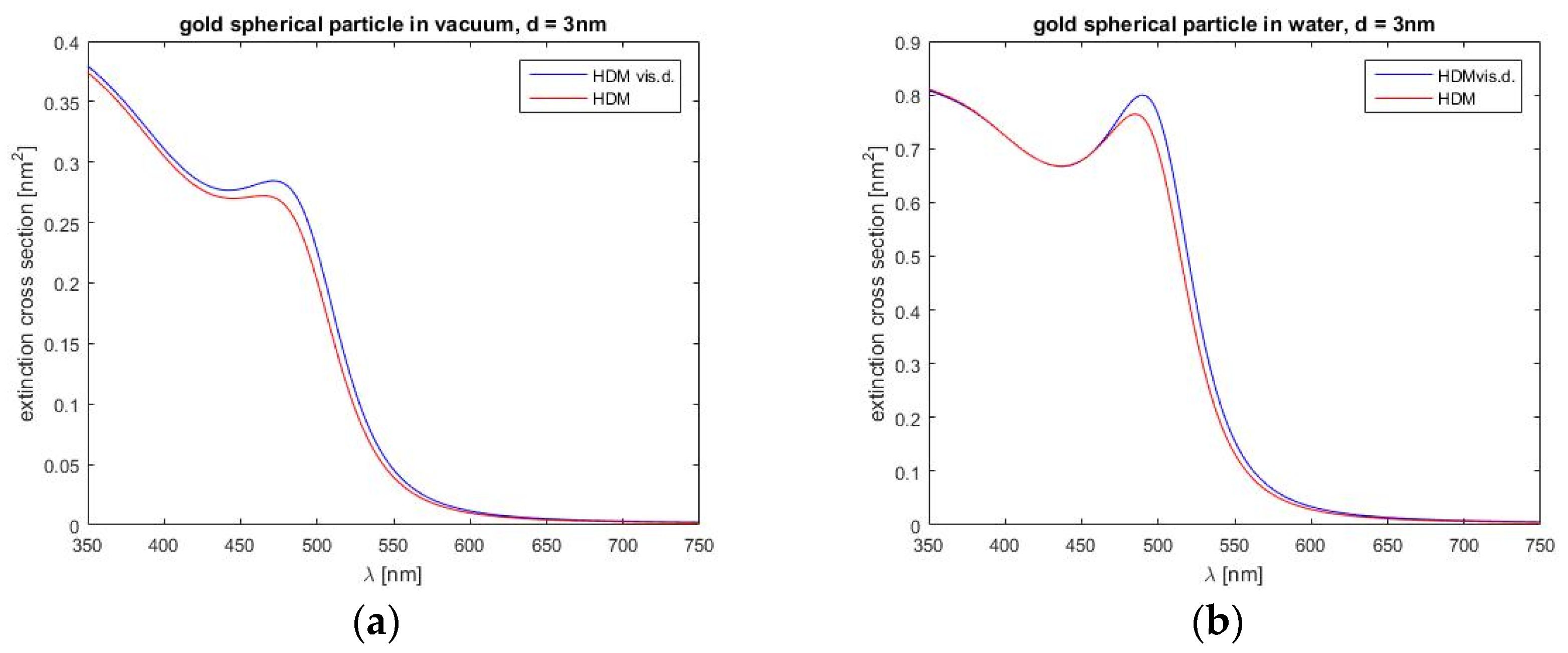
In this section, we turn to the results of the generalized HD model. From the outcome of our simulations, it is possible to come up with the following findings. First, in
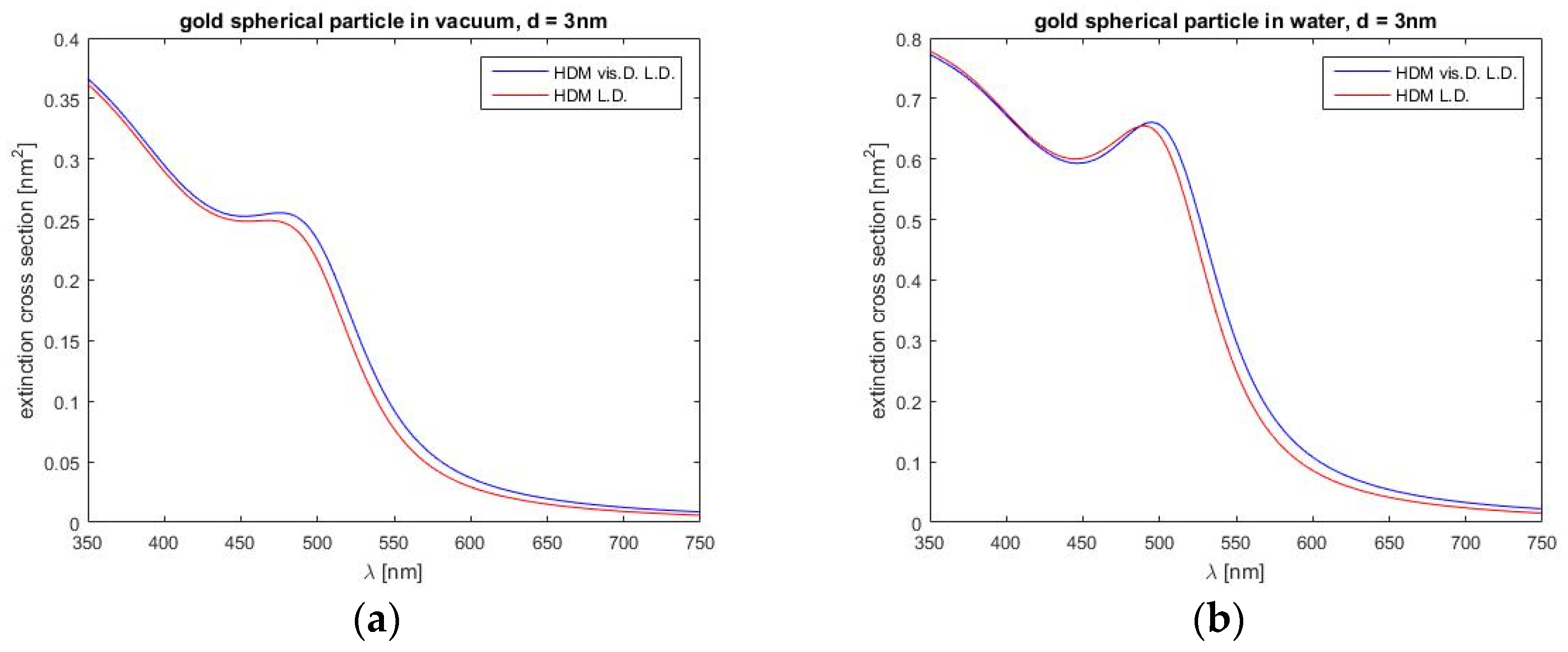
Figure 7, our viscosive damping generalization of the HDM model in comparison with the standard HDM, for a gold spherical nanoparticle, provides the extinction cross-section (standard HDM and our HDM–Vis.D. model) for a gold spherical particle (3 nm) in a vacuum (
Figure 7a) and in water (
Figure 7b). Additionally, the HDM–Vis.D. model has caused a small red correction to the blue shift of extinction local maxima (about 4 to 8 nm). Additionally, local maxima for gold spherical particles, for the smallest particles, have disappeared, in comparison with the results from the standard HDM.
This is visible in
Figure 7 where a blue curve, which represents the hydrodynamical model with viscosive damping, reaches in both cases (vacuum or water) higher values. Our model predicts a red correction to the blue shift of about 3 nm in both cases (vacuum or water), the extinction cross-section in the main resonance peak, as predicted from our model, has about a 5% higher value. Both HDM models also show that the resonance maximum is larger and narrower in the case of water surroundings. It is also seen in
Figure 7 that both models converge to the same values in the case of a water environment for shorter wavelengths (350–450 nm).
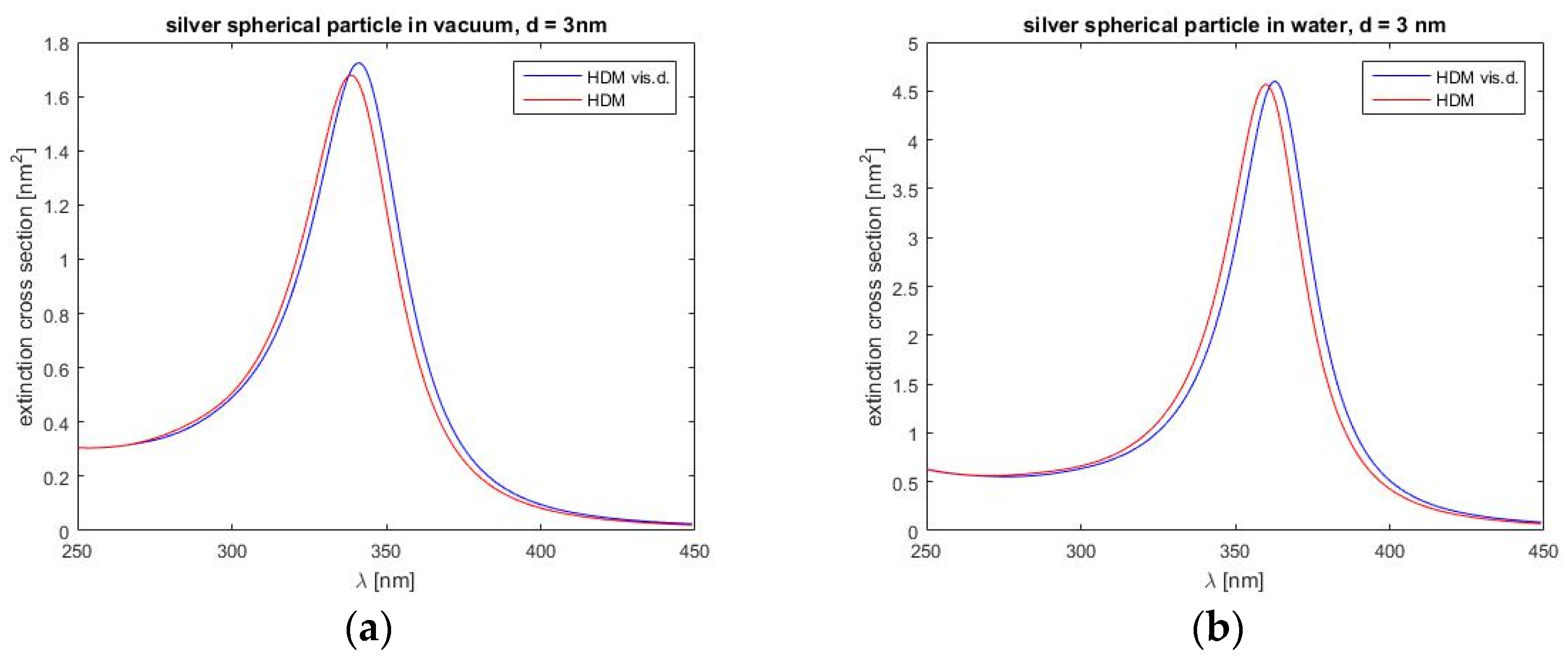
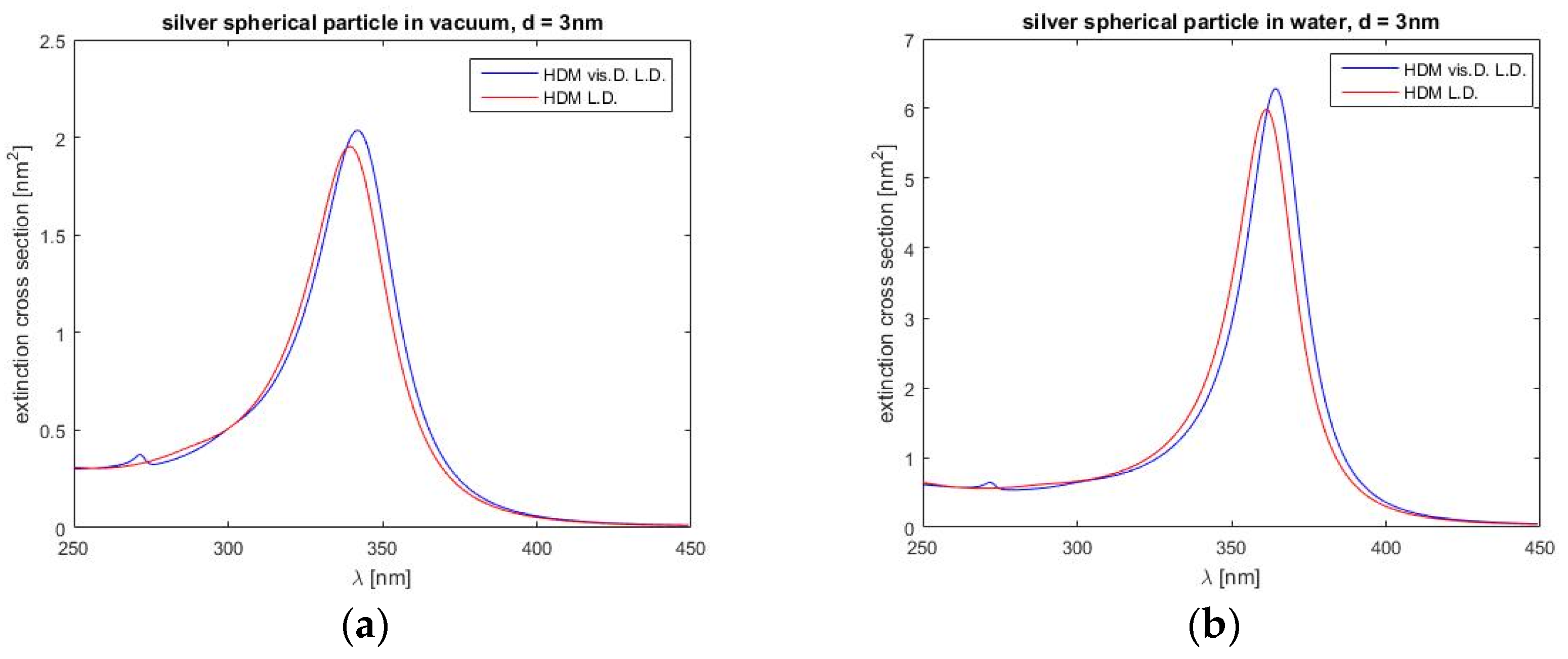
Next,
Figure 8 shows a similar comparison of both models, now for a silver spherical nanoparticle in a vacuum and a water environment. The permittivity spectral dependence is for silver obtained by the Drude–Lorentz dispersion model. In
Figure 8, we can notice again weak differences between calculated values of the two models, as expected. Similar to gold, our model again predicts a red correction to the blue shift, somewhat higher values of extinction at the resonance peak (more noticeable for a vacuum) and larger half-width values (also more obvious for a vacuum).
Further,
Figure 9 shows additional modification of calculations of the extinction spectra which are represented in
Figure 7. This modification, the Landau damping, denotes additional size-dependent damping of localized plasmons on the interface of a metal structure.
Figure 9 shows that the extinction cross-section of a gold spherical particle in a water environment has almost the same value at shorter wavelengths (between 350–400 nm), similar to
Figure 7, whereas a particle in a vacuum exhibits little difference between the two model predictions, at these short wavelengths.
The HDM model with both viscosive and Landau damping, again predicts corrections to the blue shift for both cases of surrounding environment and it also shows slightly larger values in the resonance maxima, as compared to
Figure 7. It is clearly visible that additional inclusion of Landau damping into the model causes a lowering of resonance maxima and slower convergence to zero values of the extinction cross-section for long wavelengths (up to 650 nm).
As we can see in
Figure 10, again our model with both viscosive and Landau damping, compared to the standard HDM, predicts corrections of blue shift and a slightly larger resonance maximum value. Clearly, silver particles exhibit a stronger influence of Landau damping, thus the resonance maxima peak is significantly larger and narrower (compared to
Figure 7). Descent of the extinction of the resonance wavelength up to 400 nm is surprisingly faster. Our model with viscosive and Landau damping predicts new, although very weak, resonance on shorter wavelengths. This effect may be caused by the Drude–Lorentz model for metal permittivity data.
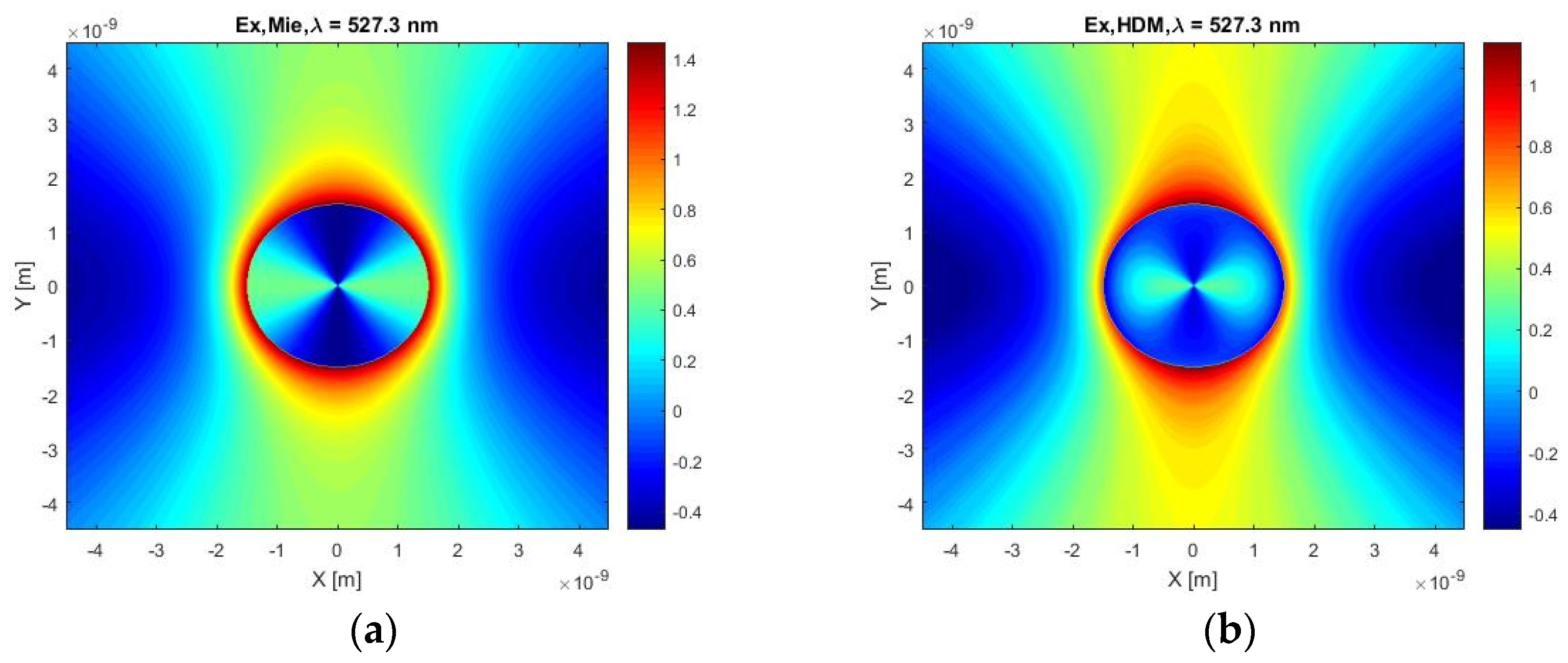
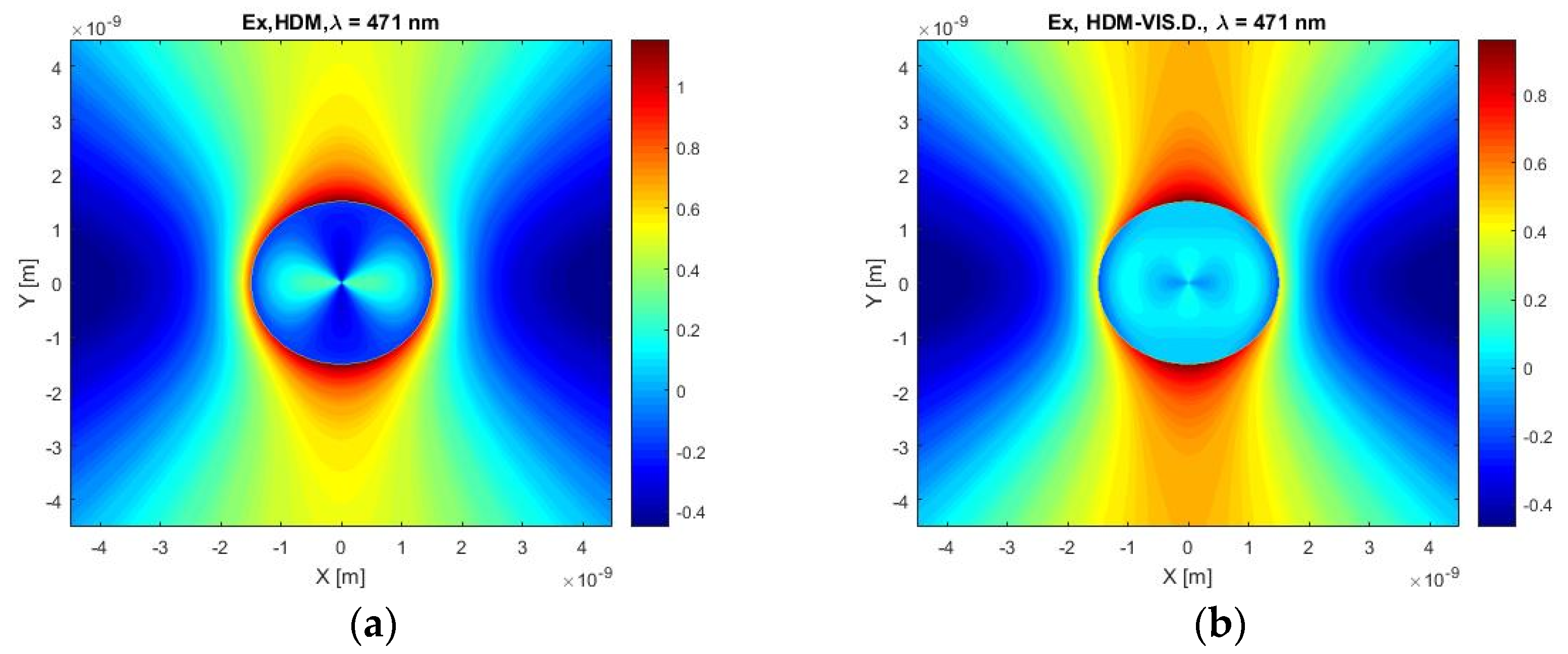
Next,
Figure 11 shows the calculated X-component of the electric field for our HDM with viscosive damping and classical HDM at the frequency of the resonant maximum of the HDM. At the first glance of the figures, a difference in the negative field values is noticeable. The calculated profile of the electric field inside a particle using HDM can help us evoke the idea of the direction of the incident plane wave, but this deduction using the field distribution in the particle calculated by HDM with viscosive damping is not so apparent.
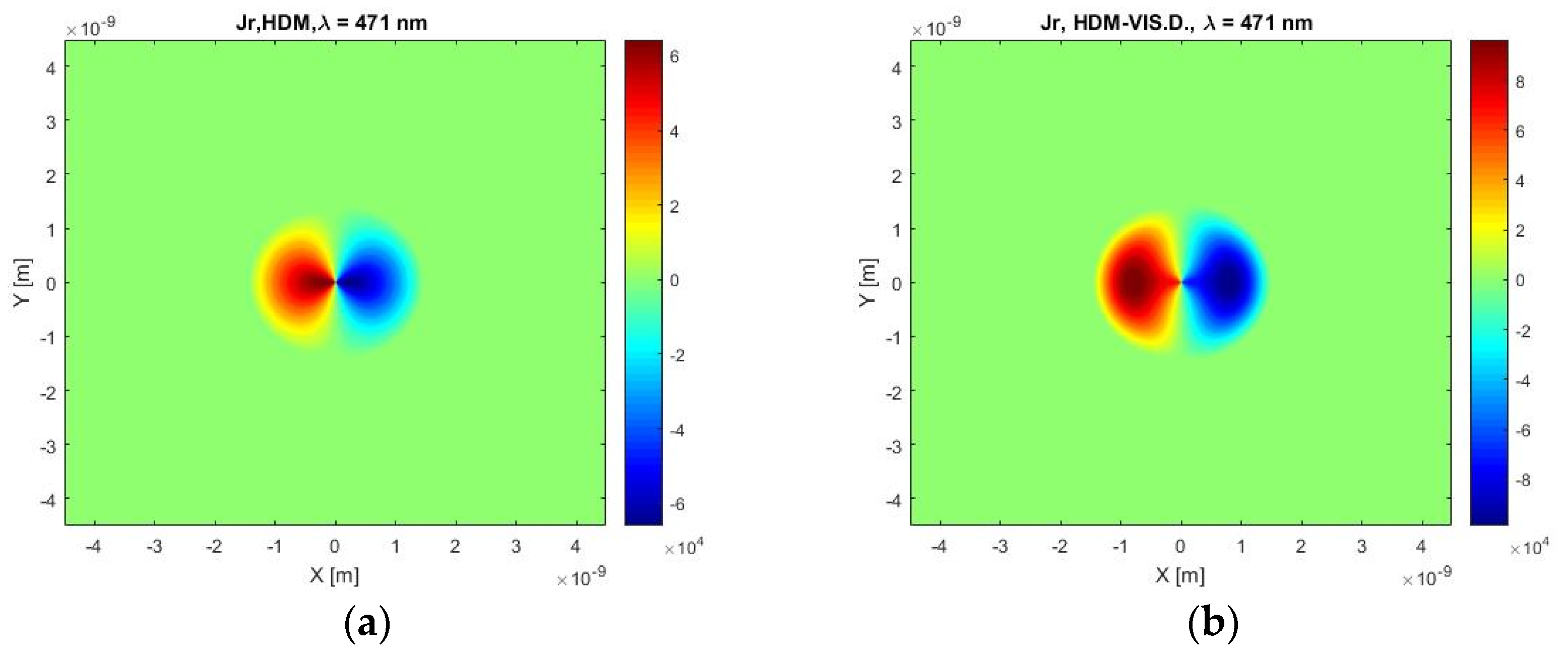
Figure 12 represents the electric current distribution in the plane cut through a spherical particle in the X and Y axes. Both graphs display a symmetric distribution of the current density in the X and Y direction. At first sight, these current profiles are very similar, but more detailed examination reveals that our HDM with viscosive damping predicts higher absolute values of the current density, and the area around the maxima value is situated away from the center of the particle (in the middle of each hemisphere) while classical HDM provides the maxima values near the center of the particle. It can be also mentioned, that classical HDM predicts a slower descent to zero values of the current density near the boundary of a particle.
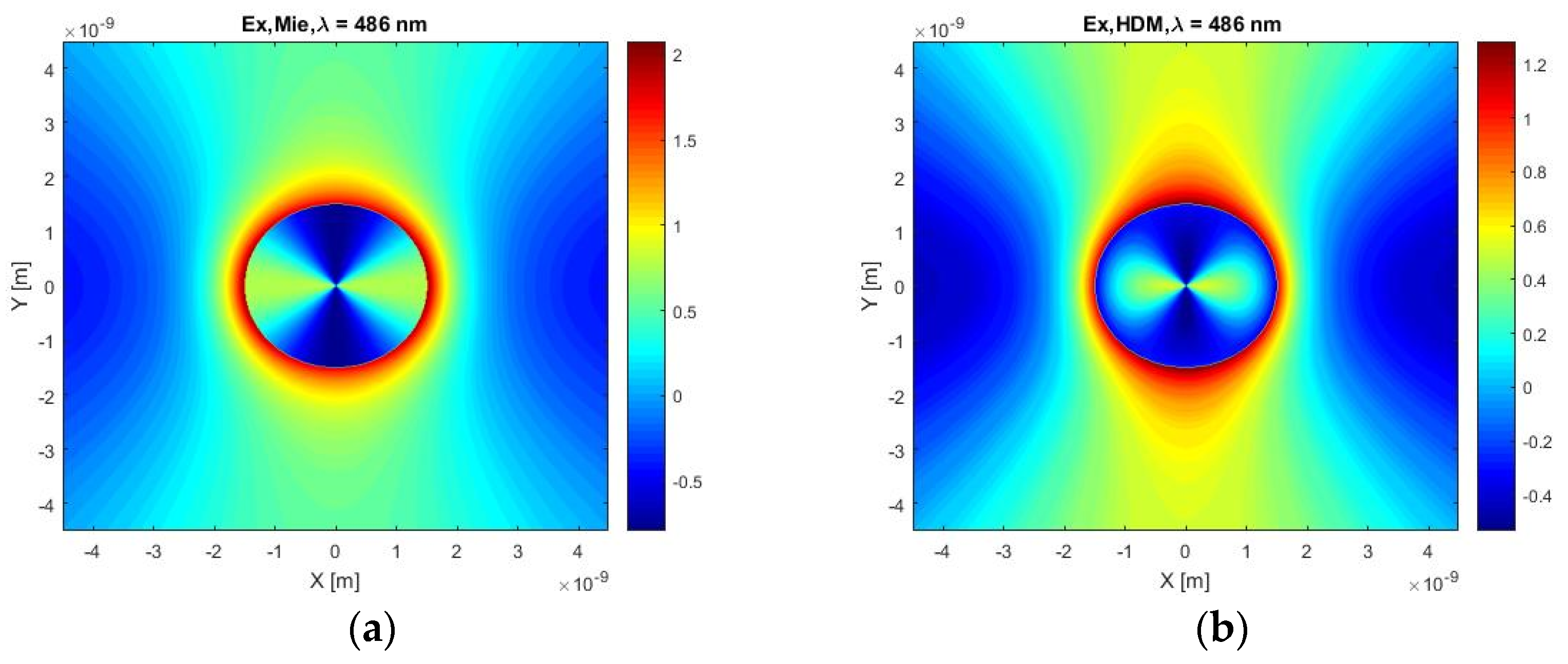
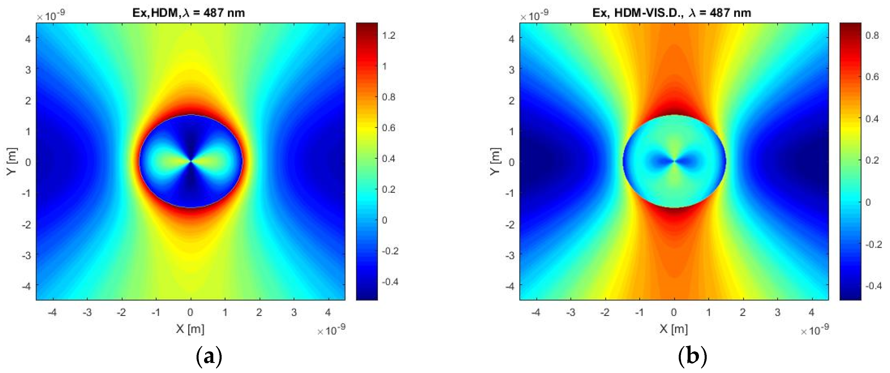
In
Figure 13, when comparing the X-component electric fields calculated by the HDM and our HDM with viscosive damping, we can notice three major differences. The first distinction is that our model predicts only a twice as strong positive maximum value than the maximum negative value, whereas the classical HDM predicts this ratio to be about three. Next, the majority of the area inside a particle exhibits an inverse value of the field, i.e., where the HDM calculations display negative values, our model shows positive values and the converse. The last difference is related to the close vicinity of a particle, in the case of the classical HDM, the particle is surrounded by a region with maximum positive values of the field, whereas positive values of the field obtained by our model are located mainly in the direction of the Y axes.
Figure 14 shows the density of the energy displayed in a plane cut that is defined by the X and Y axes. Now the reader can see, that the classical HDM predicts a larger range of the energy density values than the previous case with a vacuum environment. If we compare maximum and minimum values of the energy density within a particle, we find that the classical HDM predicts an unusually large difference in these values, moreover, there are visible areas inside the particle of a near zero density. Our model, however, predicts a different shape of distribution density of energy inside a particle and a significantly larger minimal value.
Additionally,
Figure 15 shows a very similar situation to
Figure 13, however our model predicts larger attenuation (positive maxima values) in comparison with the classical HDM.
Figure 15b, corresponding to the HDM with viscosive dumping, shows that the lowest values of the X component of the electric field are located outside the particle, whereas the HDM predicts that these values are located inside the particle and their absolute values are larger as compared to the HDM with viscosive dumping.
Next,
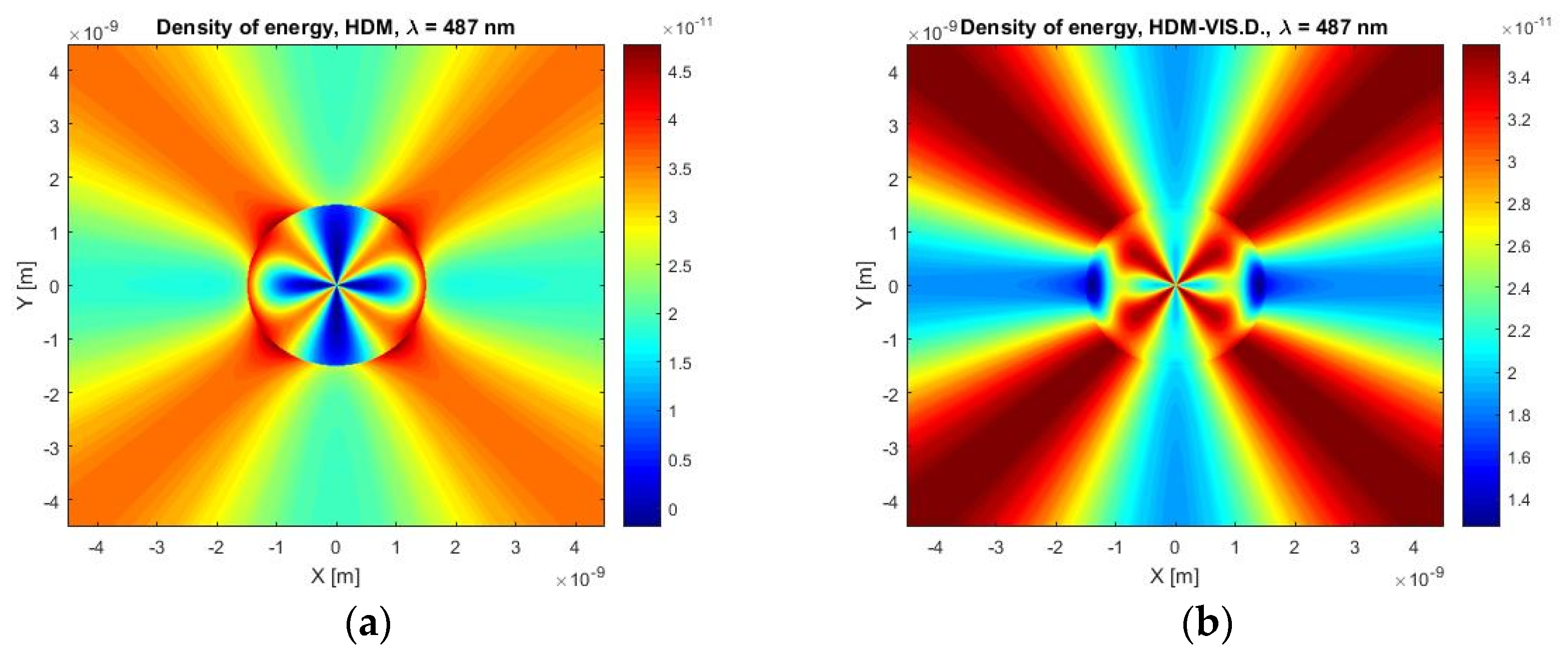
Figure 16 shows us the distribution of the energy density in the plane cut defined by the X and Y axes. Differences between the HDM and our model are clearly visible. HDM predicts that the areas with maximal energy density are located mainly inside a particle and its vicinity. It can be further read from the figures that our model predicts higher values of the lowest energy density. The lowest energy is in both cases of HD models, located inside the particle, but the area of the highest energy density calculated by our model is oriented diagonally and mainly outside of the particle.
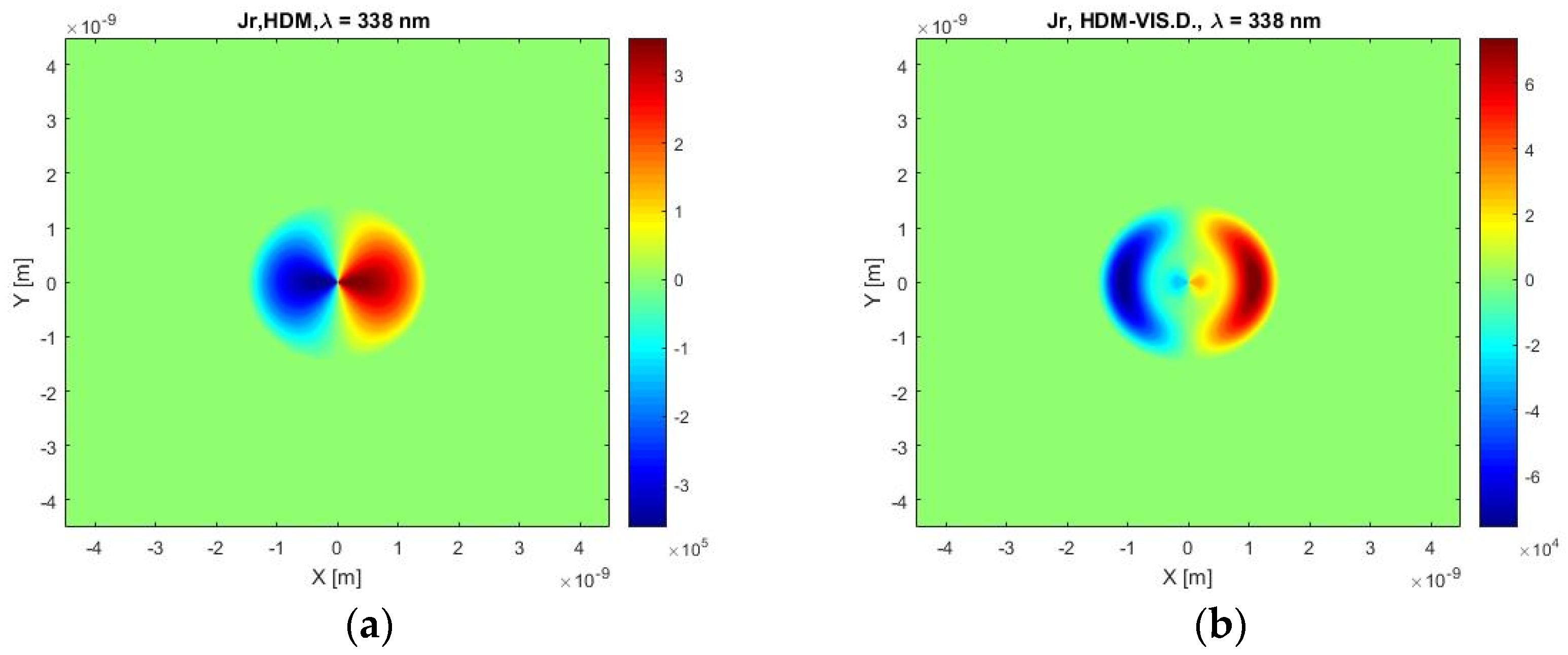
As the reader can see from
Figure 17, both models predict different distributions of the current density, but every calculated pattern is symmetric to the X axis and antisymmetric to the Y axis. A further finding from these calculations is that our model shows a two times larger current density, which is situated near the edge of the particle, whereas the area with the largest current density calculated by HDM is located near the center of the particle. Another interesting point is that our model also shows that inside a particle there is a large area where the current density is nearly zero.
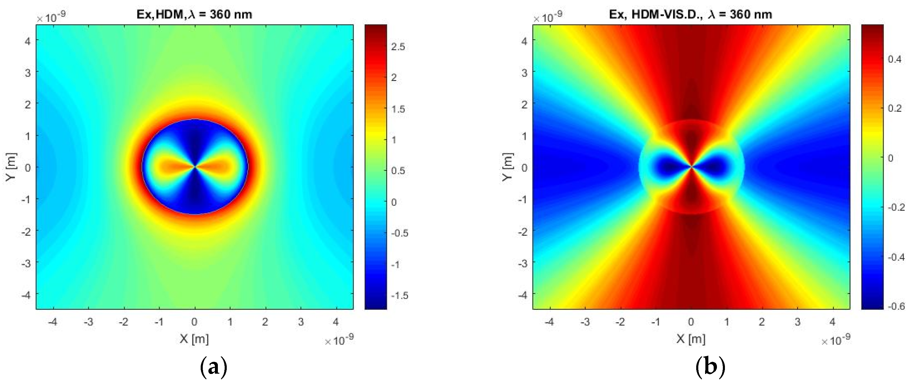
Additionally,
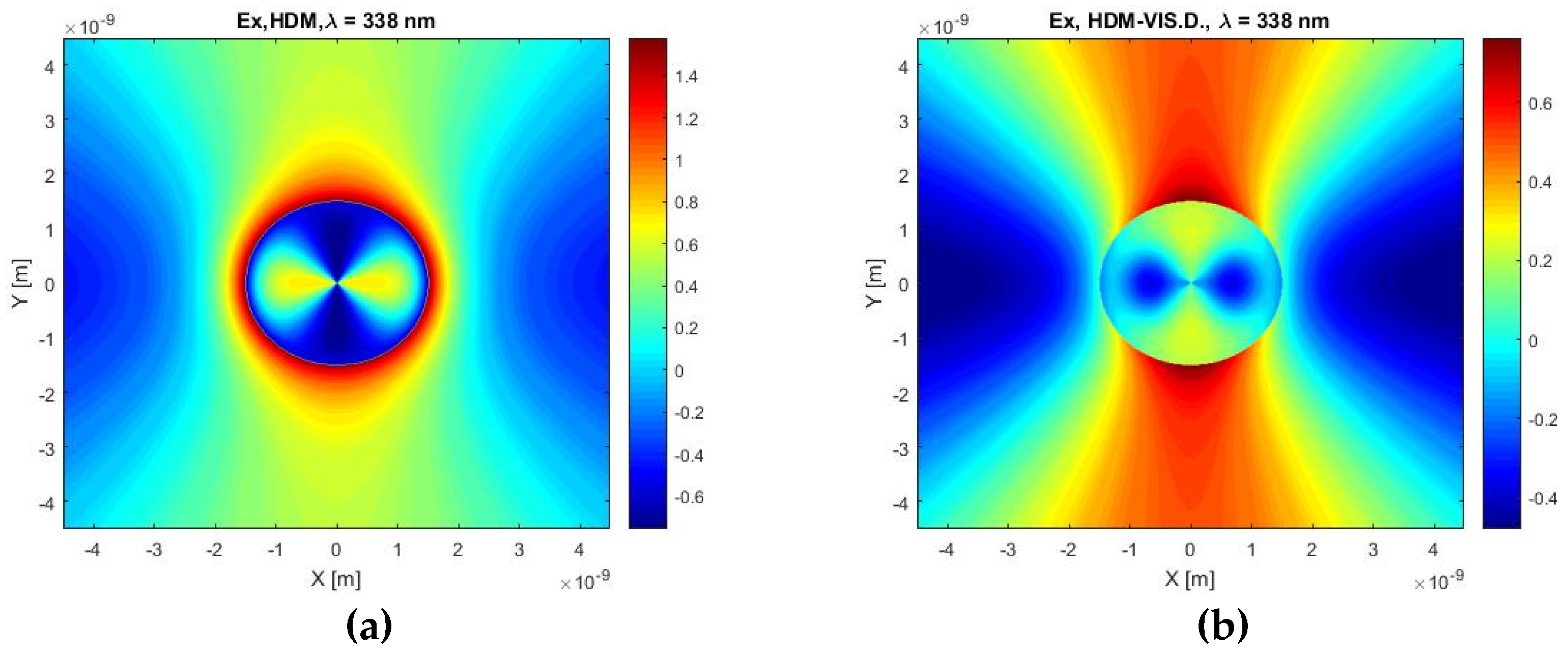
Figure 18 displays, similarly, to
Figure 16, the X-component of the electric field but for a water environment and at a different wavelength. Although these two cases are not directly comparable, we can see that the shape of the field distribution of the electric field is similar to that predicted with the HDM. In contrast to the HDM calculation, however, of our model shows the opposite distribution of positive and negative values of the electric field in a particle. Very apparent, is also a different distribution of the electric field outside of a particle, as it is determined by our model in comparison with the HDM. Again, our model predicts significantly smaller negative and positive values of the electric field.
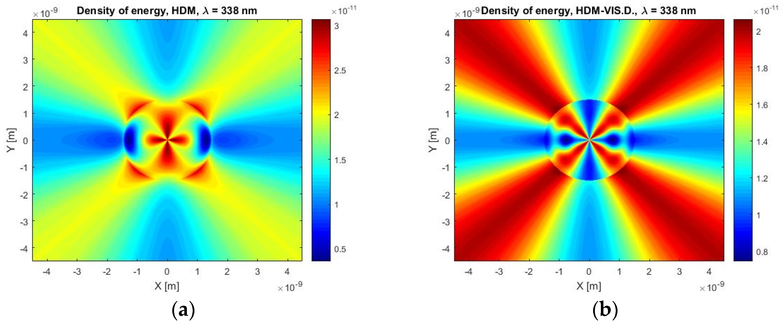
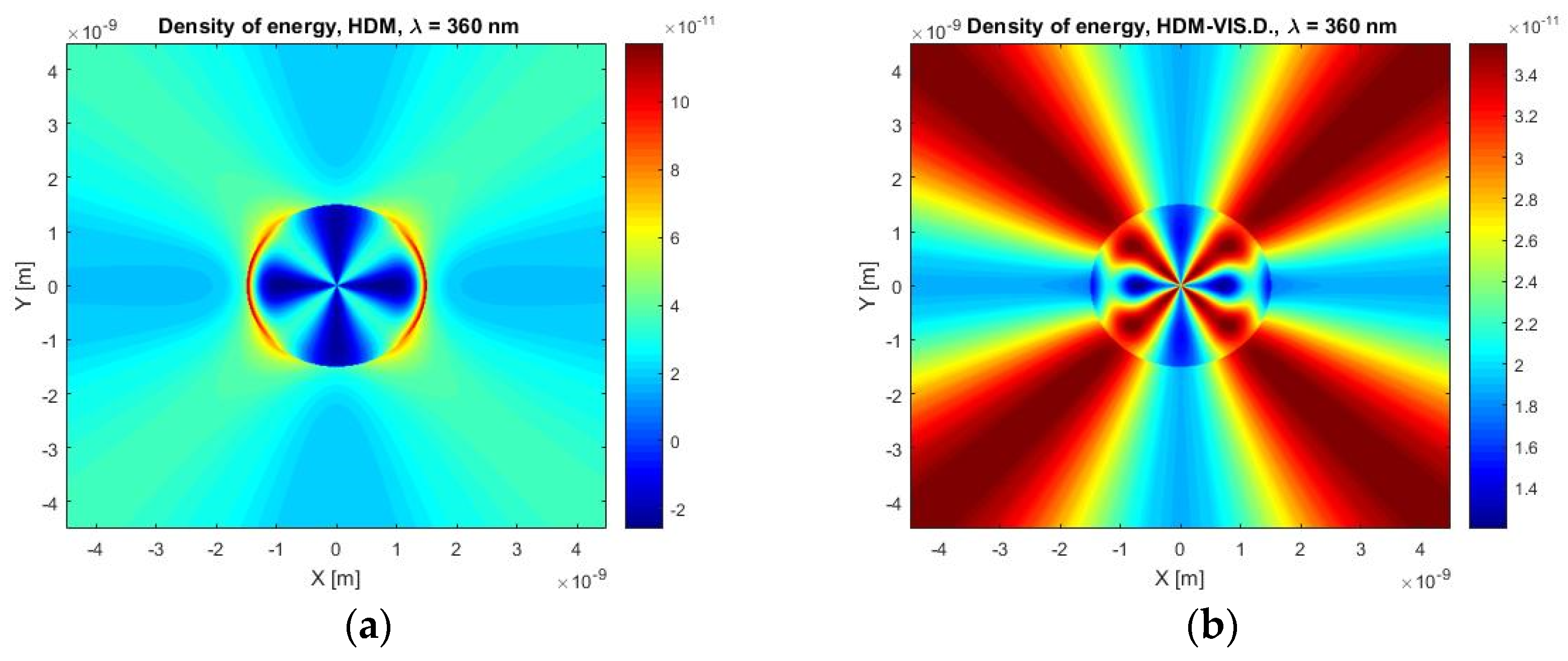
Finally,
Figure 19 shows quite important data, demonstrating another disadvantage of the classic HDM. It should be noted that the same formula was used for these calculations of energy density as for the calculations shown in
Figure 16. A quite strange finding is that standard HDM shows negative values of energy density in some places inside a particle volume; these non-physical values are not found when applying the same calculations to a gold particle. The standard HDM, unlike our model, displays large energy densities on the edge of a particle which are about three times larger than the maximum density calculated by our model. With these presented results we clearly demonstrated the applicability of our HD model with viscosive damping and generalized Drude–Lorentz term.


