Indoor Visible Light Positioning Based on Channel Estimation and Cramér–Rao Low Bound Analysis with Random Receiving Orientation of User Equipment


Abstract
:1. Introduction
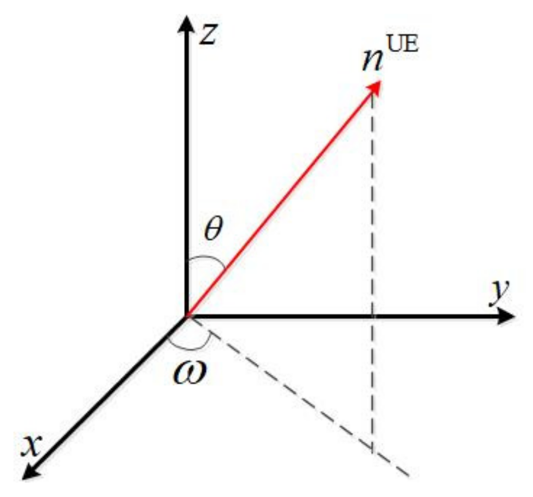
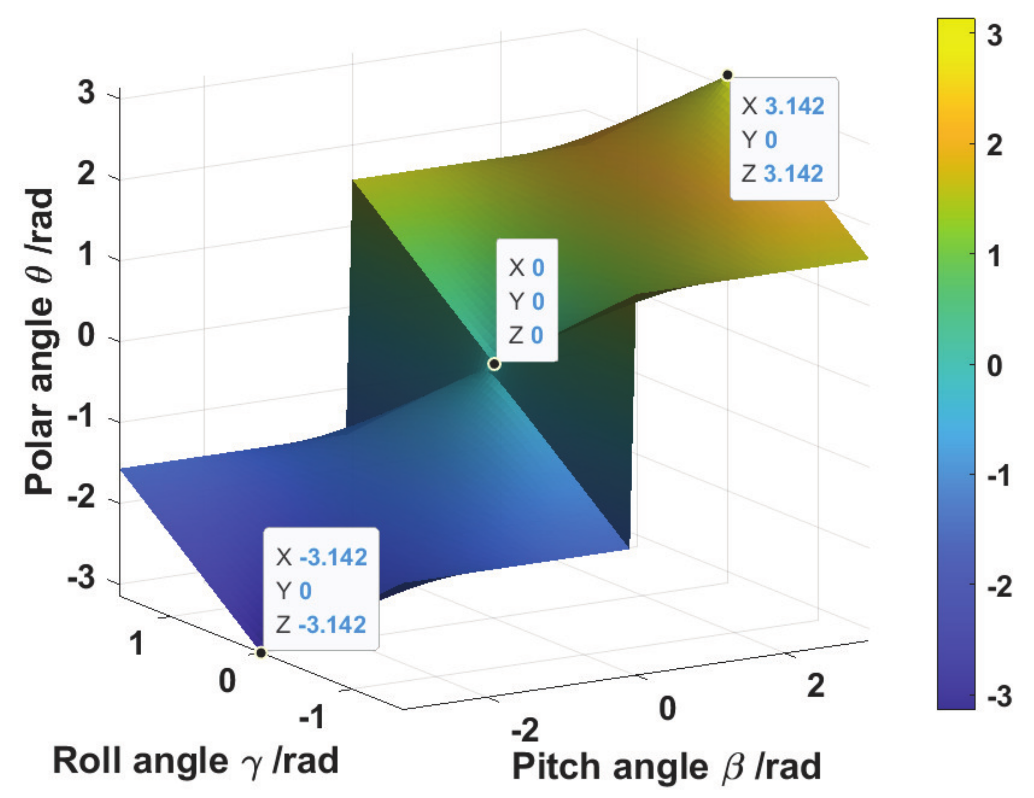
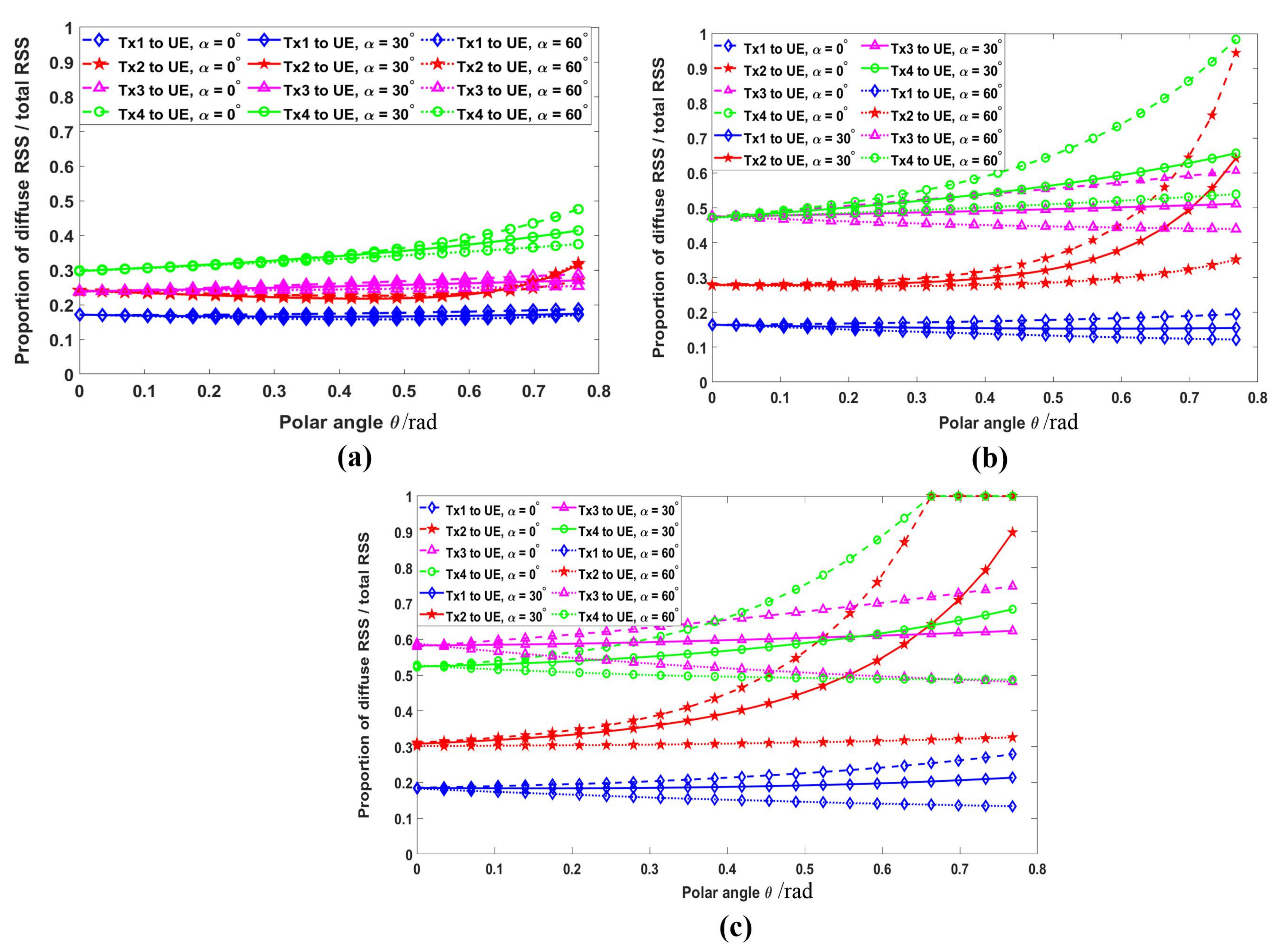
- Analysis of influence for random receiving orientation on the proportion of the diffuse component to the total received power, in which the influencing factors consist of the yaw, pitch, and roll angles;
- Proposal of a novel trilateration positioning algorithm based on channel estimation and Parseval’s theorem, which can accurately estimate the proportion of diffuse power to the total received power;
- Derivation of the CRLB for the LOS-based indoor VLP under the effect of the receiving orientation;
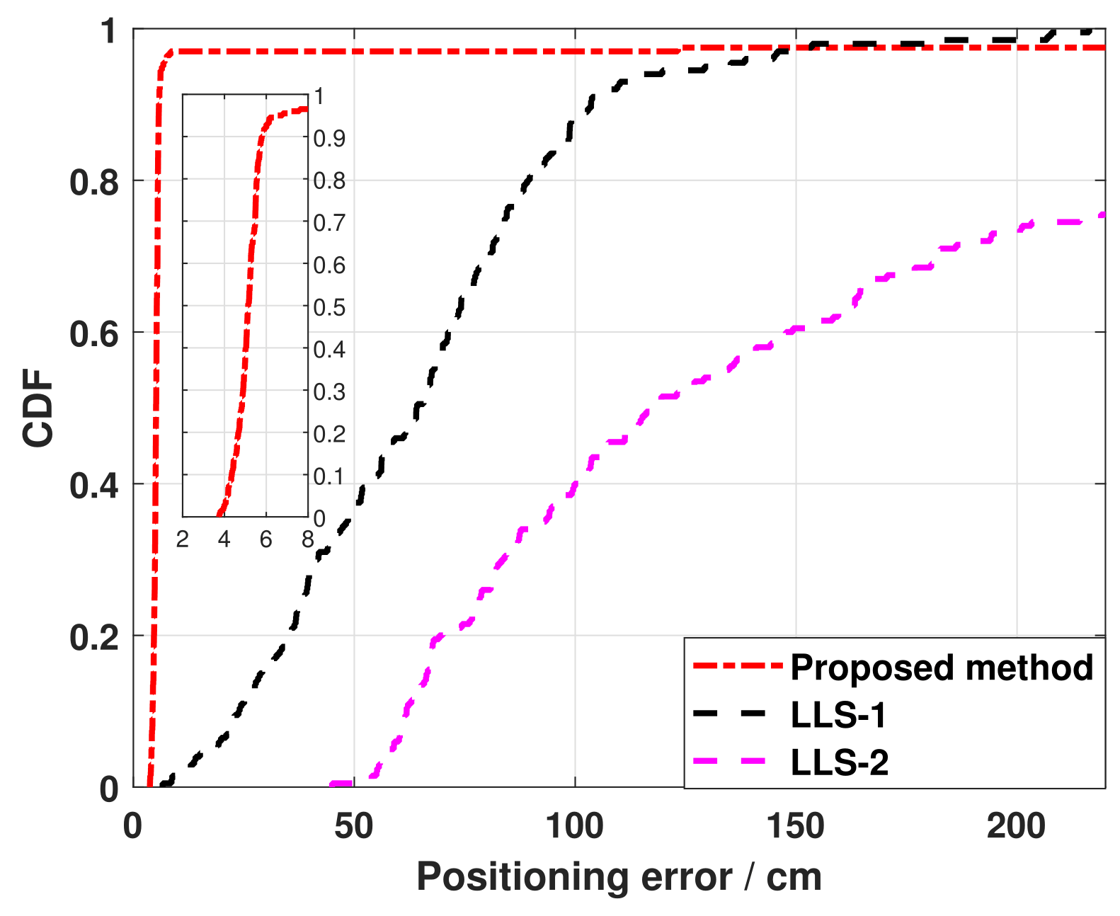
- Evaluation of the proposed positioning scheme in an actual indoor positioning scene by extensive computer simulation comparisons with the CRLB for different SNRs.
2. Channel Model for Wireless Optical Communication
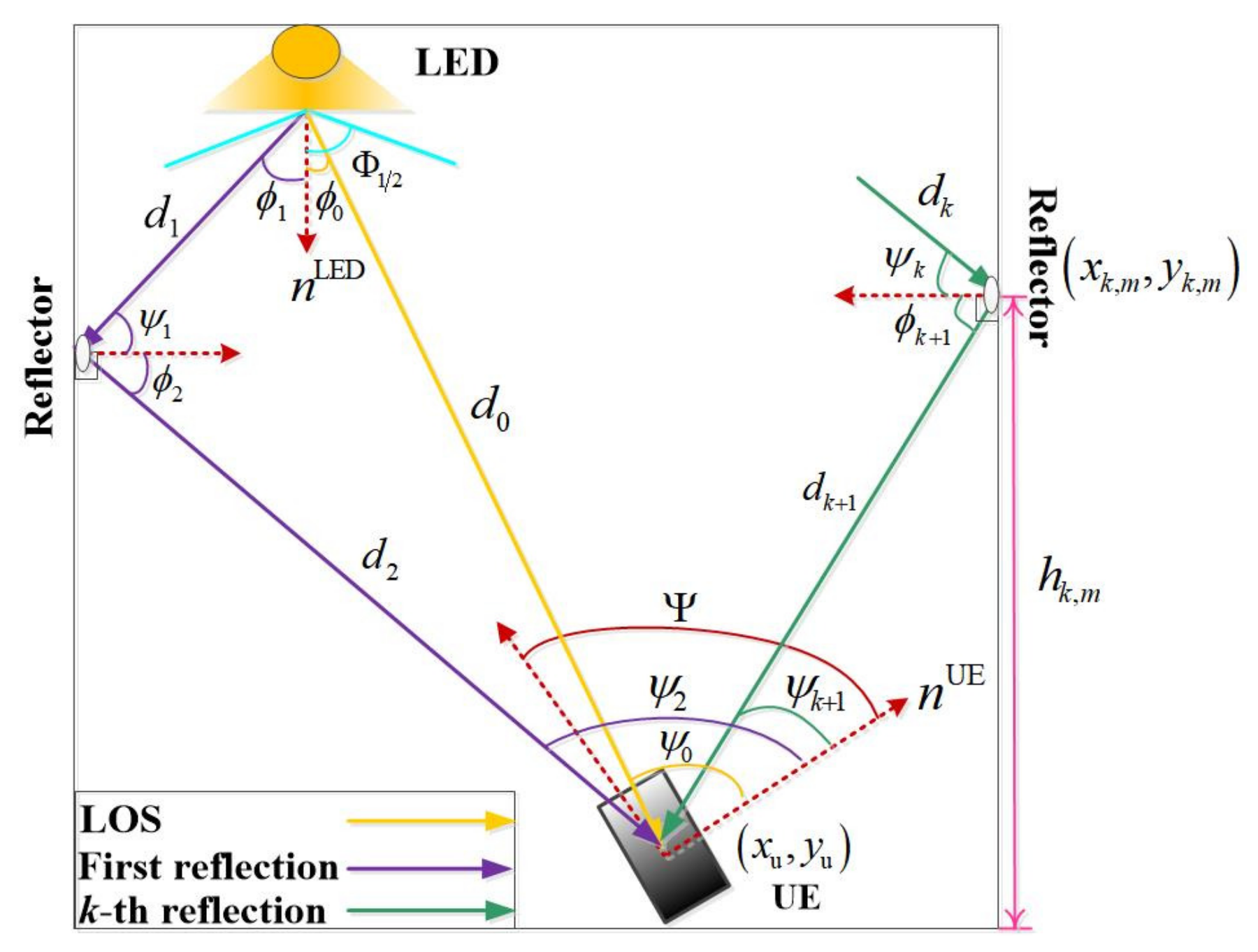
2.1. The LOS Channel
2.2. The Diffuse Channel
2.3. Overall Optical Channel
3. VLC-Based RSS Positioning System
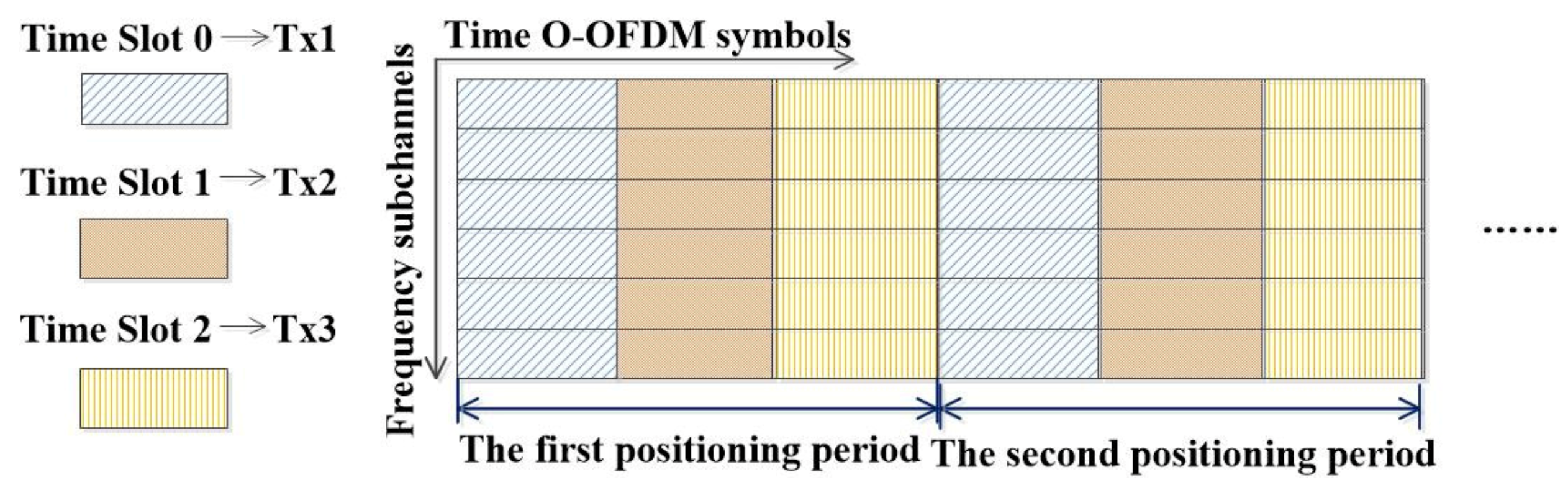
3.1. Optical OFDM–TDMA Positioning Model
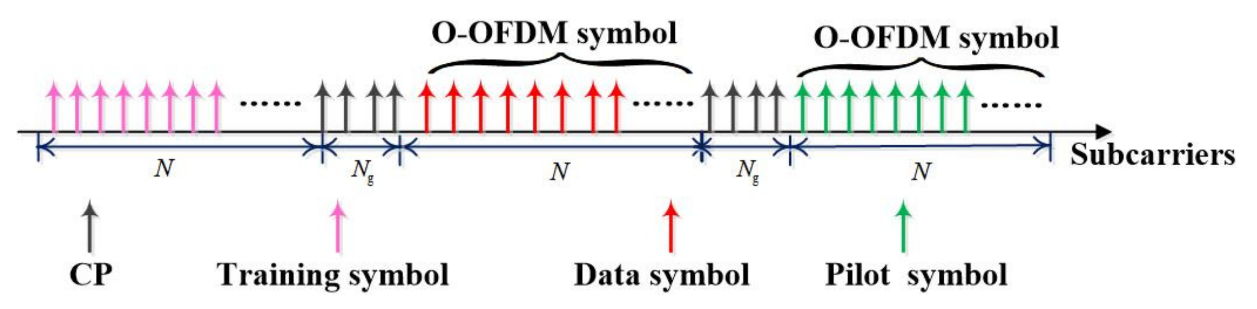
3.2. VLC-Based DCO–OFDM Transmission Strategy
3.3. Diffuse Component Elimination
| Algorithm 1 Estimation of number of channel paths based on Parseval’s theorem |
|
3.4. Position Estimation
4. Cramér–Rao Low Bound on Positioning Estimation Error
5. Discussion
6. Conclusions
Author Contributions
Funding
Institutional Review Board Statement
Informed Consent Statement
Data Availability Statement
Acknowledgments
Conflicts of Interest
References
- Chen, L.; Thombre, S.; Järvinen, K.; Alén-Savikko, A.; Leppäkoski, H.; Bhuiyan, M.Z.H.; Bu-Pasha, S.; Ferrara, G.N.; Honkala, S.; Lindqvist, J.; et al. Robustness, security and privacy in location-based services for future iot: A survey. IEEE Access 2017, 5, 8956–8977. [Google Scholar] [CrossRef]
- Maheepala, M.; Kouzani, A.Z.; Joordens, M.A. Light-based indoor positioning systems: A review. IEEE Sens. J. 2020, 20, 3971–3995. [Google Scholar] [CrossRef]
- Shirehjini, A.A.N.; Shirmohammadi, S. Improving accuracy and robustness in hf-rfid-based indoor positioning with kalman filtering and tukey smoothing. IEEE Trans. Instrum. Meas. 2020, 69, 9190–9202. [Google Scholar] [CrossRef]
- Shao, W.; Luo, H.; Zhao, F.; Tian, H.; Yan, S.; Crivello, A. Accurate indoor positioning using temporal–spatial constraints based on wi-fi fine time measurements. IEEE Internet Things J. 2020, 7, 11006–11019. [Google Scholar] [CrossRef]
- Zhu, X.; Yi, J.; Cheng, J.; He, L. Adapted error map based mobile robot uwb indoor positioning. IEEE Trans. Instrum. Meas. 2020, 69, 6336–6350. [Google Scholar] [CrossRef]
- Fang, S.H.; Wang, C.H.; Huang, T.Y.; Yang, C.H.; Chen, Y.S. An enhanced ZigBee indoor positioning system with an ensemble approach. IEEE Commun. Lett. 2012, 16, 564–567. [Google Scholar] [CrossRef]
- Huang, N.; Gong, C.; Luo, J.; Xu, Z. Design and demonstration of robust visible light positioning based on received signal strength. J. Lightw. Technol. 2020, 38, 5695–5707. [Google Scholar] [CrossRef]
- Hussain, B.; Wang, Y.; Chen, R.; Cheng, H.C.; Yue, C.P. Lidr: Visible-light-communication-assisted dead reckoning for accurate indoor localization. IEEE Internet Things J. 2022, 9, 15742–15755. [Google Scholar] [CrossRef]
- Hong, C.Y.; Wu, Y.C.; Liu, Y.; Chow, C.W.; Yeh, C.H.; Hsu, K.L.; Lin, D.C.; Liao, X.L.; Lin, K.H.; Chen, Y.Y. Angle-of-arrival (AOA) visible light positioning (vlp) system using solar cells with third-order regression and ridge regression algorithms. IEEE Photonics J. 2020, 12, 7902605. [Google Scholar] [CrossRef]
- Keskin, M.F.; Gezici, S.; Arikan, O. Direct and Two-Step Positioning in Visible Light Systems. IEEE Trans. Wirel. Commun. 2018, 66, 239–254. [Google Scholar] [CrossRef] [Green Version]
- Du, P.F.; Chen, C.; Zhong, W.D. Demonstration of a low-complexity indoor visible light positioning system using an enhanced TDOA scheme. IEEE Photonics J. 2018, 10, 7905110. [Google Scholar] [CrossRef]
- Li, Z.P.; Qiu, G.D.; Zhao, L.; Jiang, M. Dual-mode led sided visible light positioning system under multi-path propagation: Design and demonstration. IEEE Trans. Wirel. Commun. 2021, 20, 5986–6003. [Google Scholar] [CrossRef]
- Abou-Shehada, I.M.; AlMuallim, A.F.; AlFaqeh, A.K.; Muqaibel, A.H.; Park, K.H.; Alouini, M.S. Accurate indoor visible light positioning using a modified pathloss model with sparse fingerprints. J. Lightw. Technol. 2021, 39, 6487–6497. [Google Scholar] [CrossRef]
- Alam, F.; Chew, M.T.; Wenge, T.; Gupta, G.S. An accurate visible light positioning system using regenerated fingerprint database based on calibrated propagation model. IEEE Trans. Instrum. Meas. 2019, 68, 2714–2723. [Google Scholar] [CrossRef]
- Wu, Y.C.; Hsu, K.L.; Liu, Y.; Hong, C.Y.; Chow, C.W.; Yeh, C.H.; Liao, X.L.; Lin, K.H.; Chen, Y.Y. Using linear interpolation to reduce the training samples for regression based visible light positioning system. IEEE Photonics J. 2020, 12, 7901305. [Google Scholar] [CrossRef]
- Wang, K.Y.; Liu, Y.J.; Hong, Z.Y. RSS-based visible light positioning based on channel state information. Opt. Express 2022, 30, 5683–5699. [Google Scholar] [CrossRef]
- Bai, L.; Yang, Y.; Feng, C.Y.; Guo, C.L. Received signal strength assisted perspective-three-point algorithm for indoor visible light positioning. Opt. Express 2020, 28, 28045–28095. [Google Scholar] [CrossRef]
- Lee, K.; Park, H.; Barry, J.R. Indoor channel characteristics for visible light communications. IEEE Commun. Lett. 2011, 15, 217–219. [Google Scholar] [CrossRef]
- Gu, W.; Aminikashani, M.; Deng, P.; Kavehrad, M. Impact of multipath reflections on the performance of indoor visible light positioning systems. J. Lightw. Technol. 2016, 34, 2578–2587. [Google Scholar] [CrossRef] [Green Version]
- Wu, N.; Feng, L.; Yang, A. Localization accuracy improvement of a visible light positioning system based on the linear illumination of LED sources. IEEE Photonics J. 2017, 9, 7905611. [Google Scholar] [CrossRef]
- Yang, F.; Gao, J.; Liu, Y. Indoor visible light positioning system based on cooperative localization. Opt. Eng. 2019, 58, 016108. [Google Scholar] [CrossRef] [Green Version]
- Kim, H.S.; Kim, D.R.; Yang, S.H.; Son, Y.H. An indoor visible light communication positioning system using a rf carrier allocation technique. J. Lightw. Technol. 2013, 31, 134–144. [Google Scholar] [CrossRef]
- Soltani, M.D.; Purwita, A.A.; Zeng, Z.; Haas, H.; Safari, M. Modeling the random orientation of mobile devices: Measurement, analysis and lifi use case. IEEE Trans. Commun. 2018, 67, 2157–2172. [Google Scholar] [CrossRef] [Green Version]
- Arfaoui, M.A.; Soltani, M.D.; Tavakkolnia, I.; Ghrayeb, A.; Assi, C.; Safari, M.; Haas, H. Invoking deep learning for joint estimation of indoor lifi user position and orientation. IEEE J. Sel. Area Commun. 2021, 39, 2890–2905. [Google Scholar] [CrossRef]
- Mai, D.H.; Le, H.D.; Pham, T.V.; Pham, A.T. Design and performance evaluation of large-scale vlc-based indoor positioning systems under impact of receiver orientation. IEEE Access 2020, 8, 61891–61904. [Google Scholar] [CrossRef]
- Yin, L.; Wu, X.; Haas, H. Indoor visible light positioning with angle diversity transmitter. In Proceedings of the IEEE 82nd Vehicular Technology Conference, Boston, MA, USA, 6–9 September 2015; pp. 1–5. [Google Scholar]
- Abdelhady, A.M.; Amin, O.; Chaaban, A.; Shihada, B.; Alouini, M.S. Downlink resource allocation for dynamic TDMA-based VLC systems. IEEE Trans. Wirel. Commun. 2019, 18, 108–120. [Google Scholar] [CrossRef] [Green Version]
- Yang, R.X.; Ma, S.H.; Xu, Z.H.; Li, H.; Liu, X.D.; Ling, X.T.; Deng, X.; Zhang, X.; Li, S.Y. Spectral and energy efficiency of DCO-OFDM in visible light communication systems with finite-alphabet inputs. IEEE Trans. Wirel. Commun. 2022, 21, 6018–6032. [Google Scholar] [CrossRef]


| Room Parameters | Room Dimensions | |
| Reflectivity of the Walls | 0.6 | |
| Transmitter Parameters | Maximum transmitted optical power per LED | 1.5 W |
| Minimum transmitted optical power per LED | 0.5 W | |
| Number of LEDs | 4 | |
| Half power semi-angle () | ||
| Field of view of the LEDs () | ||
| Bandwidth of LED | 50 MHz | |
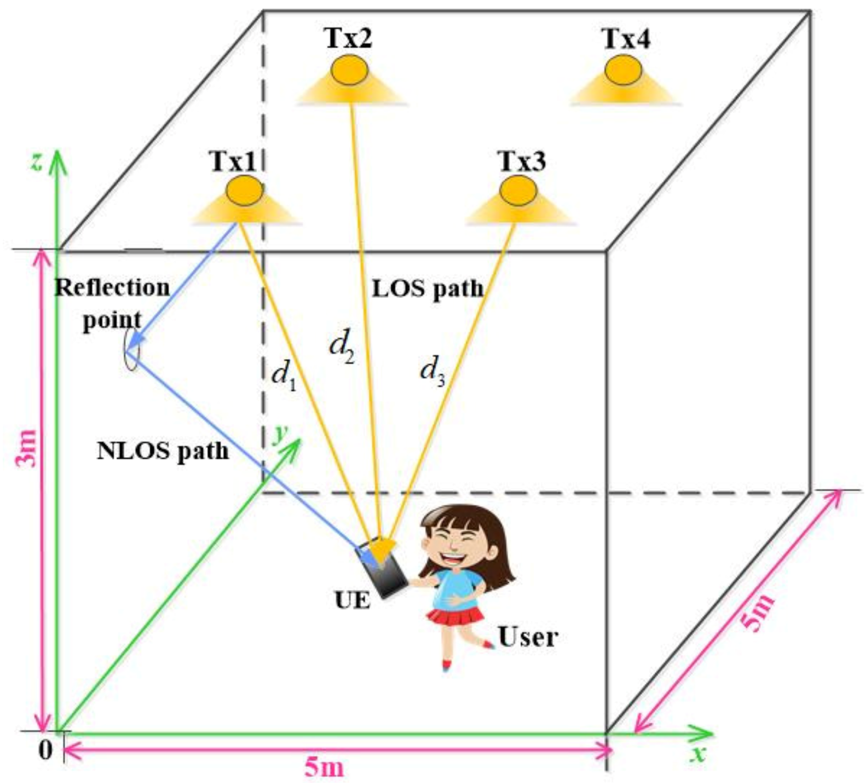
| Position of LED1 | Tx1 (−1.5, −1.5, 3) | |
| Position of LED2 | Tx2 (−1.5, 1.5, 3) | |
| Position of LED3 | Tx3 (1.5, −1.5, 3) | |
| Position of LED4 | Tx4 (1.5, 1.5, 3) | |
| Receiver Parameters | Height of UE | |
| Effective detecting area () | ||
| Gain of the optical filter () | 1 | |
| Refractive index (n) | 1 | |
| Field of view of the PDs () | ||
| Responsivity () | A/W | |
| System bandwidth (B) | 10 MHz | |
| Noise power spectral density () |
Disclaimer/Publisher’s Note: The statements, opinions and data contained in all publications are solely those of the individual author(s) and contributor(s) and not of MDPI and/or the editor(s). MDPI and/or the editor(s) disclaim responsibility for any injury to people or property resulting from any ideas, methods, instructions or products referred to in the content. |
© 2023 by the authors. Licensee MDPI, Basel, Switzerland. This article is an open access article distributed under the terms and conditions of the Creative Commons Attribution (CC BY) license (https://creativecommons.org/licenses/by/4.0/).
Share and Cite
Deng, L.; Fan, Y.; Zhao, Q.; Wu, P. Indoor Visible Light Positioning Based on Channel Estimation and Cramér–Rao Low Bound Analysis with Random Receiving Orientation of User Equipment. Photonics 2023, 10, 812. https://doi.org/10.3390/photonics10070812
Deng L, Fan Y, Zhao Q, Wu P. Indoor Visible Light Positioning Based on Channel Estimation and Cramér–Rao Low Bound Analysis with Random Receiving Orientation of User Equipment. Photonics. 2023; 10(7):812. https://doi.org/10.3390/photonics10070812
Chicago/Turabian StyleDeng, Lijun, Yangyu Fan, Qiong Zhao, and Pengfei Wu. 2023. "Indoor Visible Light Positioning Based on Channel Estimation and Cramér–Rao Low Bound Analysis with Random Receiving Orientation of User Equipment" Photonics 10, no. 7: 812. https://doi.org/10.3390/photonics10070812