Article

Influence of Image Processing Method on Wavefront Reconstruction Accuracy of Large-Aperture Laser

1
Key Laboratory of Atmospheric Optics, Anhui Institute of Optics and Fine Mechanics, Hefei Institutes of Physical Science, Chinese Academy of Sciences, Hefei 230031, China
2
Science Island Branch of Graduate School, University of Science and Technology of China, Hefei 230026, China
3
Advanced Laser Technology Laboratory of Anhui Province, Hefei 230037, China
*
Author to whom correspondence should be addressed.
Photonics 2023, 10(7), 799; https://doi.org/10.3390/photonics10070799
Submission received: 9 June 2023 / Revised: 5 July 2023 / Accepted: 6 July 2023 / Published: 10 July 2023

Abstract

:
In order to improve the wavefront reconstruction accuracy of a large-aperture laser, this paper proposed an adaptive window preprocessing algorithm based on the threshold center of gravity method (AW-TCoG). The effects of median filtering and mean filtering on spot image processing and wavefront reconstruction accuracy are simulated and analyzed. The results show that the mean filtering method has a better effect on noise elimination and can further improve the accuracy of wavefront reconstruction. In addition, the centroid detection errors of large-aperture laser wavefront reconstruction through the center of gravity (CoG), the threshold center of gravity (T-CoG), and the Windowing method were studied. The analysis shows that, due to the influence of noise, the wavefront reconstruction accuracy is poor when the CoG and Windowing methods are used to calculate centroid parameters, while the wavefront reconstruction accuracy of the threshold centroid method is better and can reach 0.2λ. When using the AW-TCoG proposed in this paper, the wavefront reconstruction accuracy can be maintained within 0.1λ for different incident wavefront RMS values and spot images with different signal-to-noise ratio (SNR) levels. Compared with the traditional threshold centroid method, the wavefront reconstruction accuracy of this method is significantly improved.

1. Introduction

The beam quality of large-aperture lasers is difficult to measure directly. Therefore, the laser at the exit of the system can be measured by constructing a lens array suitable for the laser beam size, so as to obtain the beam quality parameters [1,2,3]. In the practical application scene, due to the influence of ambient light, detector noise, and other factors, the sub-aperture spot intensity distribution in the spot image collected using the detector array is uneven [4,5], which leads to a decrease in spot centroid positioning accuracy, thus affecting the wavefront reconstruction accuracy and beam quality parameter measurement accuracy [6,7,8].
In order to solve the problem of centroid localization of spot images in a lens array, researchers have proposed a series of methods in recent years. The accuracy of centroid detection is improved by improving centroid location algorithms, such as CoG, T-CoG, weighted center of gravity (W-CoG), correlation algorithm (CORR), etc. [9,10,11]. The pixel values of the spot image are directly processed via spatial filtering, such as mean filtering, median filtering, etc. [12,13]. However, the above method has a poor filtering effect on the image and low calculation accuracy of the centroid when the SNR of the spot image is low [14]. In addition, the centroid extraction method based on a neural network is also widely used, but the centroid positioning accuracy of this method depends on the training set generation method and model training accuracy. When the near-field light intensity of the incident beam fluctuates dynamically, the training set generation is complicated and the model training is more difficult, so it is difficult to use in the actual complex wavefront detection scene at present [15,16,17,18].
In order to further improve the centroid positioning accuracy of the spot in the lens array, this paper compares and analyzes the traditional centroid calculation method. Firstly, the median filter and mean filter are used to preprocess the spot, and the resulting images obtained using the two methods are compared. Then, CoG, T-CoG, and Windowing methods are used to calculate the centroid parameters of the spot. The results show that when the image SNR is poor, the accuracy of wavefront reconstruction is low by using the above method to calculate the centroid parameters. Therefore, this paper proposed an adaptive window preprocessing algorithm based on the threshold center of gravity method (AW-TCoG). That is, after using the filtering algorithm to process each spot, windows are added according to the spot intensity distribution in each image, and then T-CoG is used to calculate the centroid of the image in the window. The simulation results show that the reconstruction accuracy of the wavefront is greatly improved when this method is used to calculate the centroid parameters of spot images at different SNR levels.

2. System Structure and Parameter Measurement Methods

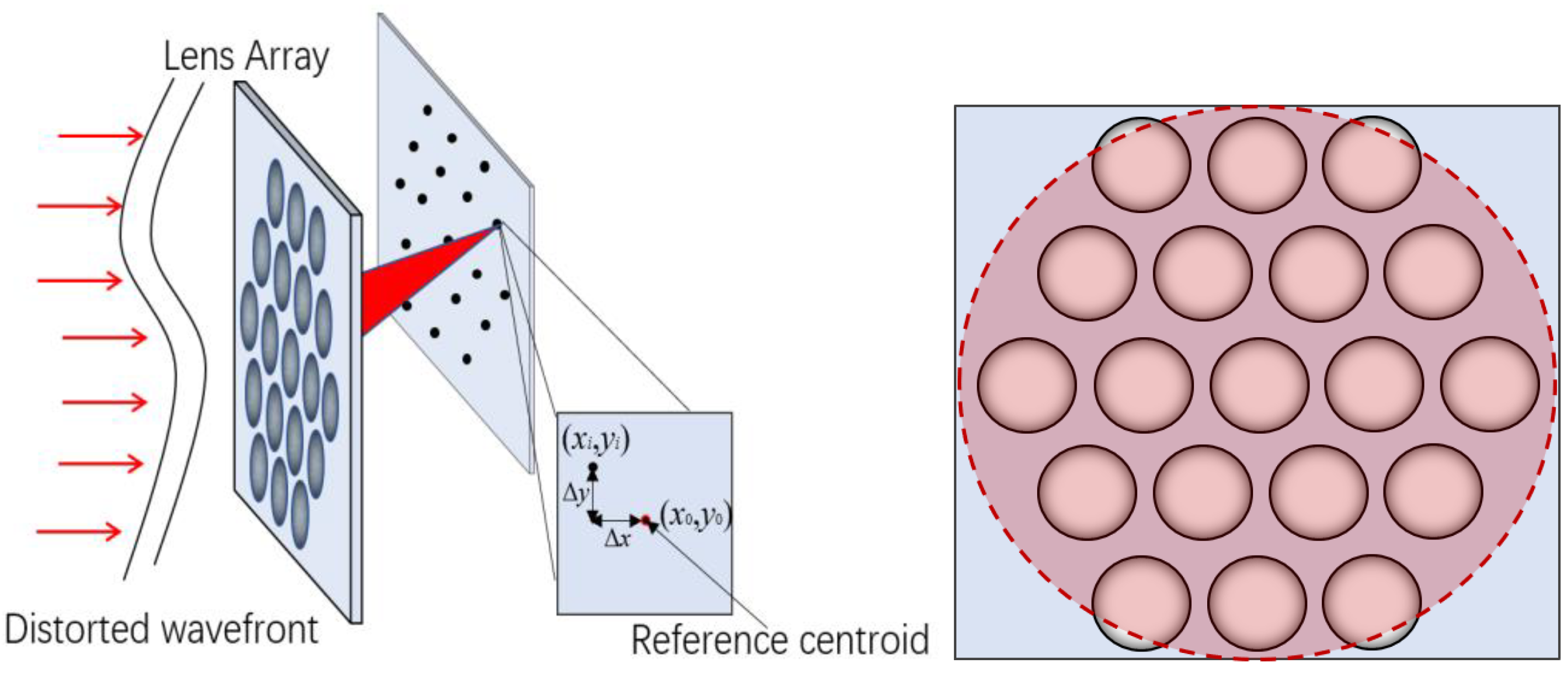
2.1. System Structure

The wavefront distribution of a large-aperture laser beam can be measured using the lens array method [19,20]. This method is different from the traditional Hartmann wavefront sensor in that the lens elements are not connected. By adjusting the lens size and lens spacing, the near-field detection of a large-aperture beam at the system exit is realized. The key in wavefront reconstruction is the offsetting of centroid coordinates. According to the offset, the wavefront slope within each sub-lens region can be obtained, and then the wavefront shape of the incident beam can be reconstructed through a wavefront reconstruction algorithm [21,22,23]. The system structure and lens arrangement are shown in Figure 1. The red area in the figure is the effective detection range of the incident beam, and Table 1 is the system parameters.
The slopes in the x and y directions of the corresponding local wavefront on the sub-aperture are gxi and gyi, respectively. The calculation formula is as follows:
g x i = Δ x i f g y i = Δ y i f
Therefore, gxi and gyi can be obtained by measuring Δxi and Δyi. After calculating gxi and gyi, the corresponding algorithm can be used to reconstruct the wavefront phase of the incident beam.

2.2. Wavefront Reconstruction Algorithm

The commonly used wavefront reconstruction methods in adaptive optics include the region method and Zernike mode method [24]. The wavefront phase distribution can be expressed by Zernike polynomials [25]:
Φ ( x , y ) = k = 1 l a k z k ( x , y )
where l is the number of modes, a k is the coefficient of the kth Zernike polynomial, and z k is the kth Zernike polynomial.
The wavefront reconstruction calculation of the Zernike mode method can be expressed in the form of a matrix as:
G x ( 1 ) G y ( 1 ) G x ( 2 ) G y ( 2 ) G x ( m ) G y ( m ) = Z x 1 ( 1 ) Z x 2 ( 1 ) Z x N ( 1 ) Z y 1 ( 1 ) Z y 2 ( 1 ) Z y N ( 1 ) Z x 1 ( 2 ) Z x 2 ( 2 ) Z x N ( 2 ) Z y 1 ( 2 ) Z y 2 ( 2 ) Z y N ( 2 ) Z x 1 ( m ) Z x 2 ( m ) Z x N ( m ) Z y 1 ( m ) Z y 2 ( m ) Z y N ( m ) a 1 a 2 a N
where m is the total number of lens elements and N is the number of Zernike polynomials; ZxN(m) and ZyN(m) are the average wavefront slope of the Nth Zernike polynomial in the mth lens region in the x and y directions, respectively, which can be simplified as:
G = Z     A
Here, G is the calculated wavefront slope matrix, Z is the 2 m × N reconstruction matrix, and A is the Zernike polynomial coefficient matrix that we need to calculate. The specific solution of matrix A can be achieved using a matrix operation. In general, twice the total number of lenses is larger than the number of Zernike terms, so the singular value decomposition method can be used to calculate the generalized inverse matrix Z+ of Z. Matrix A is given by
A = Z +   G
After the coefficient matrix is calculated, the wavefront can be reconstructed by substituting it back into Formula (2).
In this paper, we used the root mean square error (RMSE) as the standard to measure the accuracy of the wavefront reconstruction. The RMSE represents the root mean square value of the wavefront residual; the smaller the value, the higher the accuracy of the restoration. The phase information of a residual wavefront is obtained by subtracting the reconstruction wavefront and the incident wavefront, and then the RMS is calculated. The calculation formula is:
ε RMSE = ( u ( ϕ ( u ) ϕ o ( u ) ) 2 ) / N
where ϕo(u) is the original wavefront, ϕ(u) is the recovery wavefront, and N is the total number of sampling points.

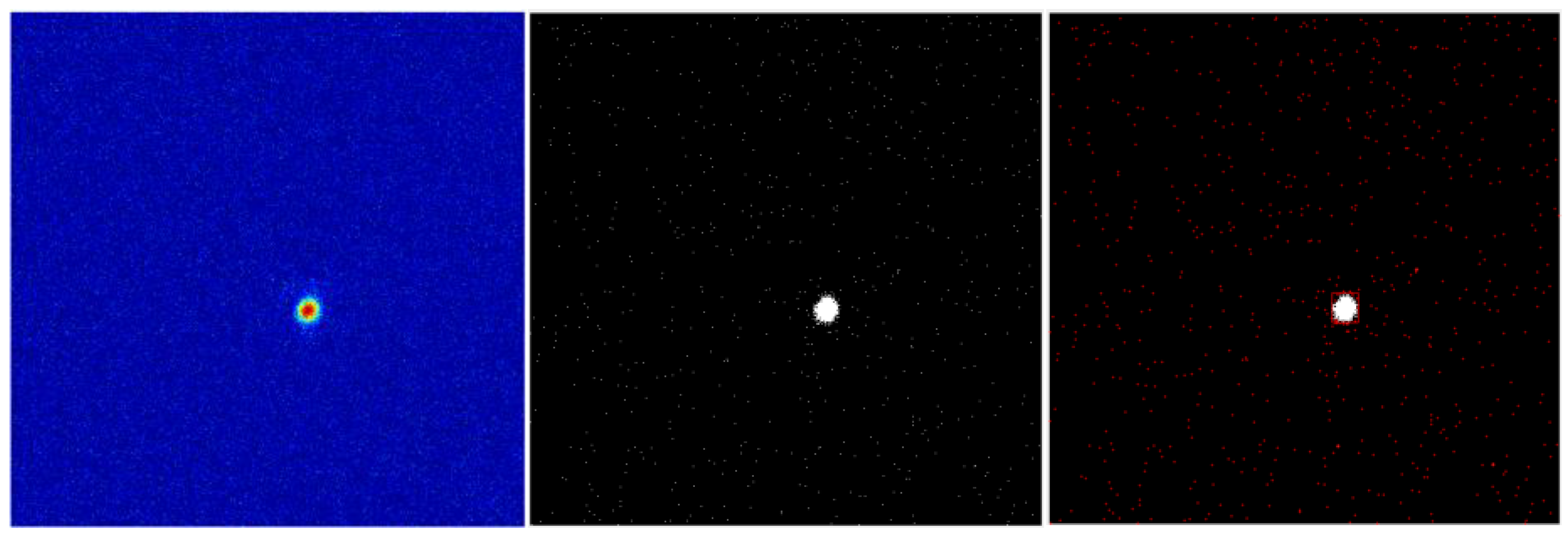
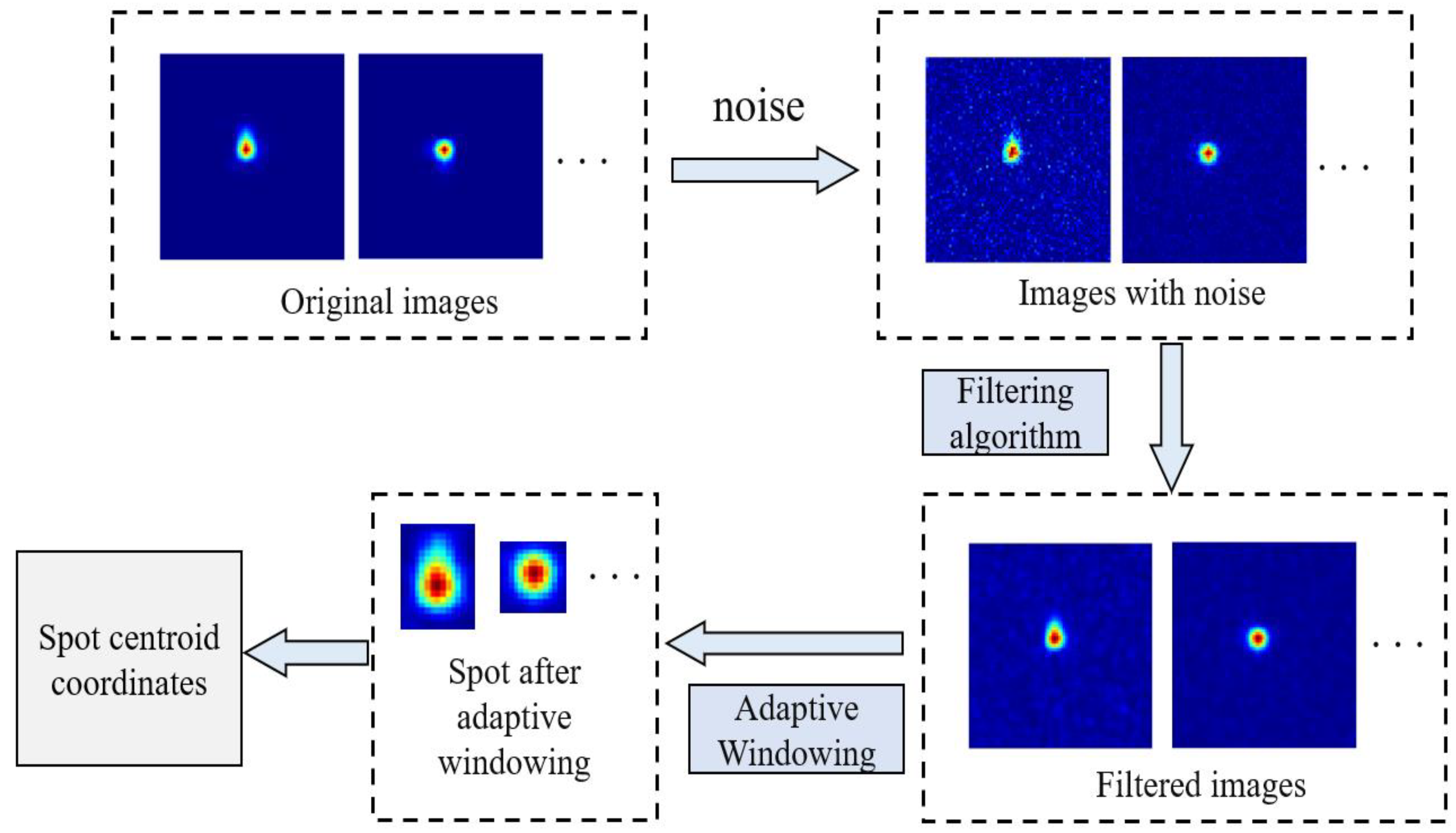
2.3. Filtering Method

Mean filtering and median filtering are two commonly used image filtering methods, so this paper focuses on the analysis of these two filtering methods. Mean filtering, also known as linear filtering, mainly uses the geometric neighborhood averaging method [12]. The basic principle of mean filtering is to use the current pixel and several neighborhood pixels to form a template and calculate the mean of all pixels in the template to replace the current pixel value in the original image. The same processing is performed on each pixel in the image to form a new image after processing.
Assuming that the original image is f(x, y) and the template size is 3 ∗ 3 (its size and shape depend on the actual needs), the processed image f′(x, y) can be expressed as
f ( x , y ) = 1 3 3 i = 1 1 j = 1 1 f ( x + 1 , y + 1 )
The mean filter using the neighborhood averaging method is very suitable for removing the particle noise in the image obtained via scanning, but it also causes blurring due to averaging, and the blurring degree is proportional to the neighborhood radius.
Median filtering is a commonly used nonlinear smoothing filter. Its basic principle is to replace the value of a point in the image with the median value of each point in a neighborhood of the point. Let {f(x, y)} denote the gray value of each point in the image. The two-dimensional median filter with window size S can be defined as:
f ( x , y ) = M e d { f ( x + s , y + t ) , ( s , t ) S ( x , y ) }
Its main function is to change the pixel with a large difference in gray value from the surrounding pixel to a value close to the surrounding pixel value, thereby eliminating isolated noise points. Therefore, median filtering is very effective for filtering salt-and-pepper noise in images.

2.4. Centroid Algorithm

For the calculation of the centroid of the spot image, the CoG, the T-CoG, and the Windowing method are widely used. The centroid method can be regarded as a weighted operation of the gray value of the target image, which can be expressed using Formula (9).
x 0 = i = 1 M j = 1 N i f ( i , j ) i = 1 M j = 1 N f ( i , j ) F F S k , S S y 0 = i = 1 M j = 1 N j f ( i , j ) i = 1 M j = 1 N f ( i , j )
where m and n represent the total number of pixels in the horizontal and vertical directions, respectively, and f(i,j) represents the gray value of the (i,j)th pixel.
When the image centroid is calculated using the CoG, the central information of the target image is not fully utilized, which results in the weak anti-noise ability of the method. If the noise increases, the accuracy will be seriously reduced. Therefore, the CoG method requires a high-SNR image to meet the accuracy requirements [26].
The Windowing method applies a window to the sub-aperture spot image. For the noise outside the window, the windowing method can effectively reduce its influence on the centroid detection accuracy, thereby improving the centroid detection accuracy. The location and size of the window will affect the extraction results of the effective information of the spot, which will affect the accuracy of the spot centroid calculation. Therefore, when using the Windowing method, it is particularly important to select the appropriate window size.
The T-CoG method can remove some noise in the grayscale image, but the appropriate threshold should be determined according to the background characteristics of the local area of the target image point in the actual image. If the threshold is too large, part of the target image information will be lost, resulting in asymmetry in the gray distribution of the target image, causing a large error. If the threshold is too small, more noise will remain. It can be seen from Reference [27] that the optimal value of the threshold is the mean of the spot image intensity plus 3-times the RMS value of the noise.
x 0 = i = 1 M j = 1 N i   [ f ( i , j ) T ] i = 1 M j = 1 N [ f ( i , j ) T ] F F S k , S S y 0 = i = 1 M j = 1 N j   [ f ( i , j ) T ] i = 1 M j = 1 N [ f ( i , j ) T ]
where T is the set threshold.
When the noise intensity is large or the noise has a great influence on the spot shape, it is difficult to achieve high-precision calculation of the spot centroid by using the T-CoG method. Therefore, this paper proposes the AW-TCoG. Firstly, each spot is processed using the filtering method. Since the shape of the spot in each sub-aperture focal plane is different after the distorted wavefront passes through the lens array, the algorithm adds a window based on the spot intensity distribution of each spot and then calculates the centroid of the spot using the T-CoG method in the added window.
According to the formula, 2.44 λ / d , the diffraction limit angle of the beam passing through a single lens can be known, and the spot size in the focal plane of the detector can be determined according to the double-diffraction limit angle.
D = 2.44 λ d f
As shown in Figure 2, the image is binarized using the global threshold method. Then, the white area in the binary image is surrounded by a frame, and the window size (a, b) for windowing the spot image can be obtained, where a and b represent the length and width of the added window, respectively. In addition, it should be noted that due to the threshold processing of the spot image, the final calculated window size of each sub-spot is also different, so the value of (a, b) needs to be compared with the theoretically calculated spot size D. In order to ensure that more of the effective information on the spot is retained in the window, a larger value is selected.
A i = a i   ,   a > D D   ,   a < D   ,     B i = b i   ,   b > D D   ,   b < D
here, i is the number of spots to be measured, and Ai and Bi represent the length and width of each window finally determined.
The approximate positions of the centroid in the spot image calculated using Formula (9) are ( x i , y i ) . Taking ( x i , y i ) as the center coordinates of the added window, the window with a size of Ai × Bi is added, respectively. Finally, the centroid coordinate parameters of the image to be detected in the added window are obtained using the threshold method. Figure 3 shows a diagram of the adaptive spot windowing threshold centroid method.

3. Numerical Simulation

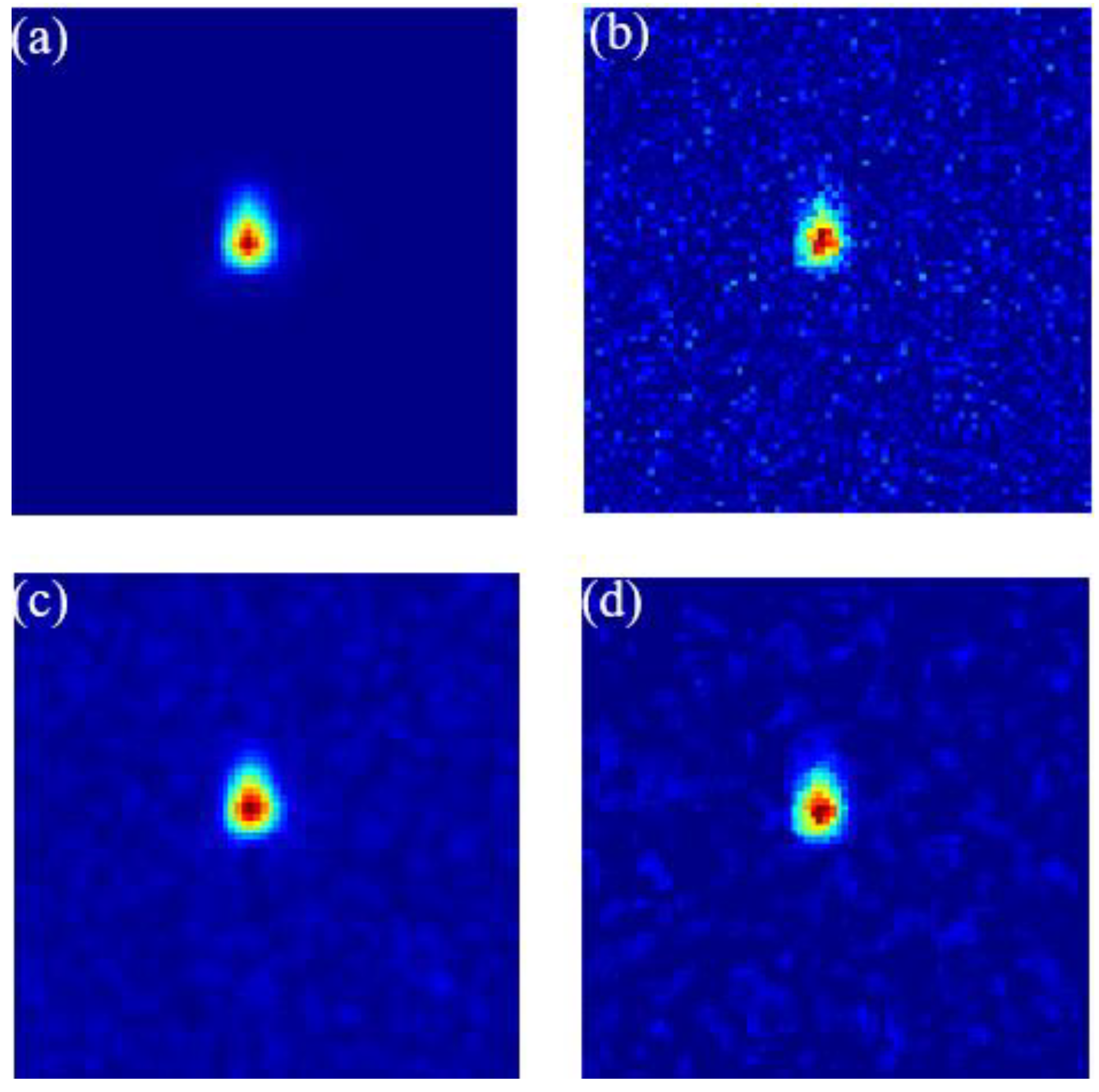
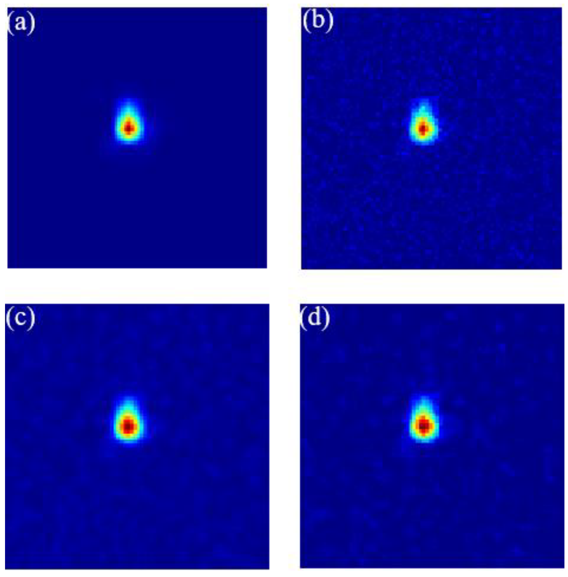
3.1. Image Filtering

When the detector collects the sub-spot image, it will introduce signal photon noise, background photon noise, readout noise, and so on due to the influence of the environment and the quantum characteristics of the photodetector [17,18]. According to the characteristics of detection noise, the noise of the photodetector is generally represented by the Poisson–Gaussian model. In this model, the signal-related noise introduced by the quantum characteristics of the sensor is modeled via Poisson distribution, and the signal-independent noise is modeled via Gaussian distribution [19,20]. The formula is as follows:
s ( x ) = a · p ( s 0 ( x ) ) + n ( x )
where s(x) is the image with noise, s0(x) is the clear image, x is a pixel, a is the gain, n is the Gaussian noise distribution with mean value m and standard deviation σ, and p is the Poisson noise distribution depending on the signal. By adjusting the signal light intensity or noise level, different SNR images can be obtained. The SNR of a single sub-aperture image can be expressed as:
R S N m = ( u = 1 N v = 1 N I u v N 2 μ n ) / ( N 2 σ n ) R S N p = ( I max μ n ) / σ n R S N e = 20 log [ ( u = 1 N v = 1 N I u v N 2 μ n ) / σ n ]
where R S N m , R S N p , and R S N e are the mean SNR, peak SNR, and energy SNR of the sub-aperture, respectively, Iuv is the gray value at the pixel (u, v), Imax is the maximum gray value in the sub-aperture, μn is the mean value of the noise in the sub-aperture, σn is the root mean square value of the noise in the sub-aperture, and N is the width of the approximate Airy spot. In this paper, SNRm is used to represent the mean value of SNR of all sub-apertures. Figure 4 shows 100 random wavefront aberrations generated according to Formula (2).
According to Formula (13), noise is added to the wavefront to obtain noise images at different SNR levels. The noise image is processed using mean filtering, median filtering, and non-filtering, respectively, and then the centroid of the image is extracted using the threshold centroid method. The wavefront is reconstructed using the Zernike mode method, and then the wavefront reconstruction accuracy is calculated using Formula (6). Figure 5 and Figure 6 represent two cases of high and low SNR in image filtering, respectively. Figure 5 indicates that the SNRm is 5, and Figure 6 indicates that the SNRm is 12. The wavefront reconstruction accuracy obtained using the above three methods of noise image processing is shown in Figure 7.
Combined with Figure 5 and Figure 6, we can draw the following conclusions: when the SNR of each sub-aperture is low, the noise has a great influence on the spot, and the mean filtering method has a relatively good effect on noise elimination. When the SNR of each sub-aperture is high, the influence of noise on the spot shape is small. At this time, the mean filtering or median filtering method has a similar effect on noise elimination. It can be seen from Figure 7 that the accuracy of wavefront reconstruction is relatively high when only the T-CoG method is used to calculate the centroid. If the noise image is preprocessed using mean filtering, the accuracy of wavefront reconstruction can be further improved. The median filter is less effective for noise filtering that does not belong to the salt-and-pepper noise type; specifically, when the image SNR is low, it will lead to a decrease in the accuracy of wavefront reconstruction. In summary, this paper chooses the mean filtering method to process the image globally.

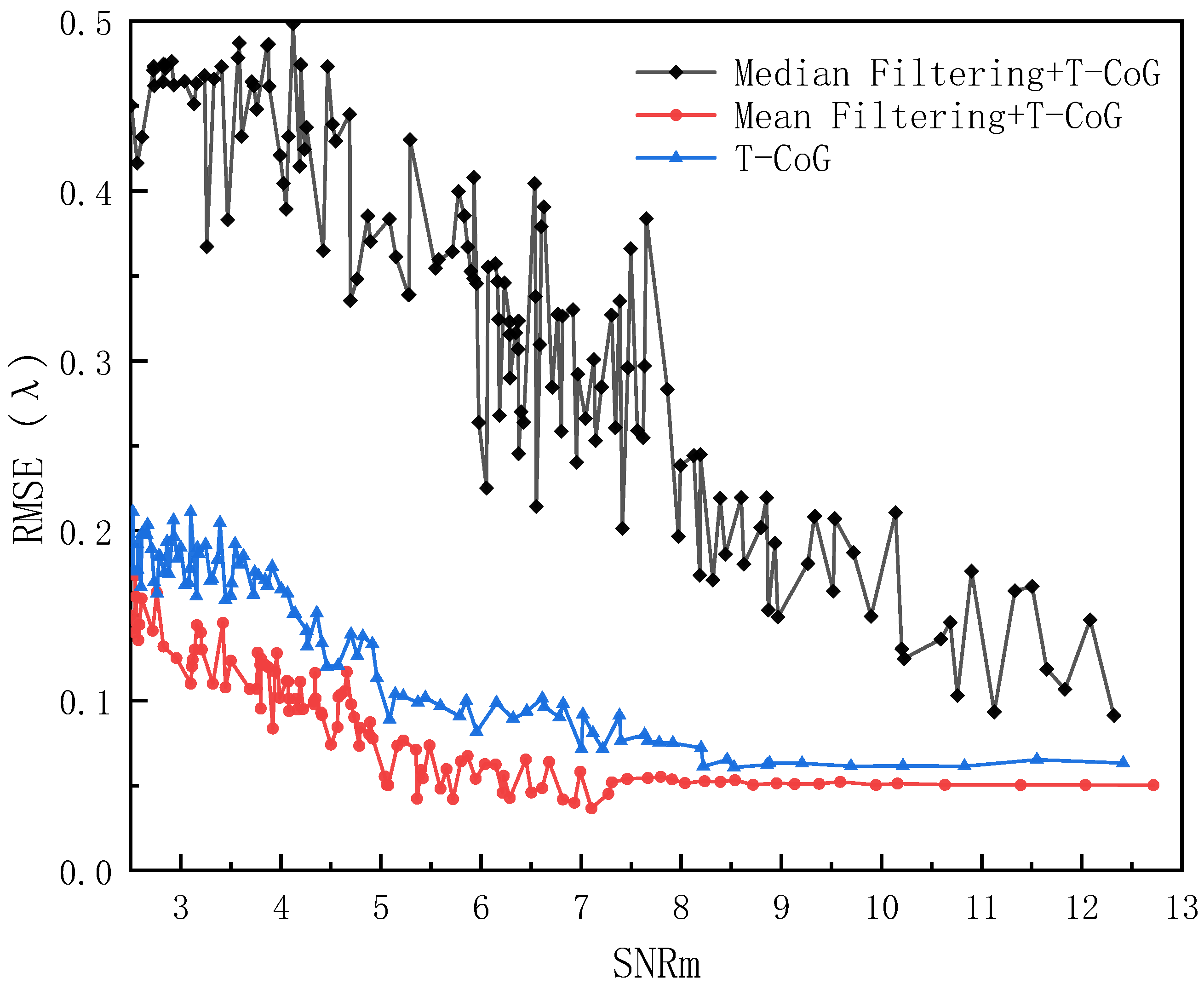
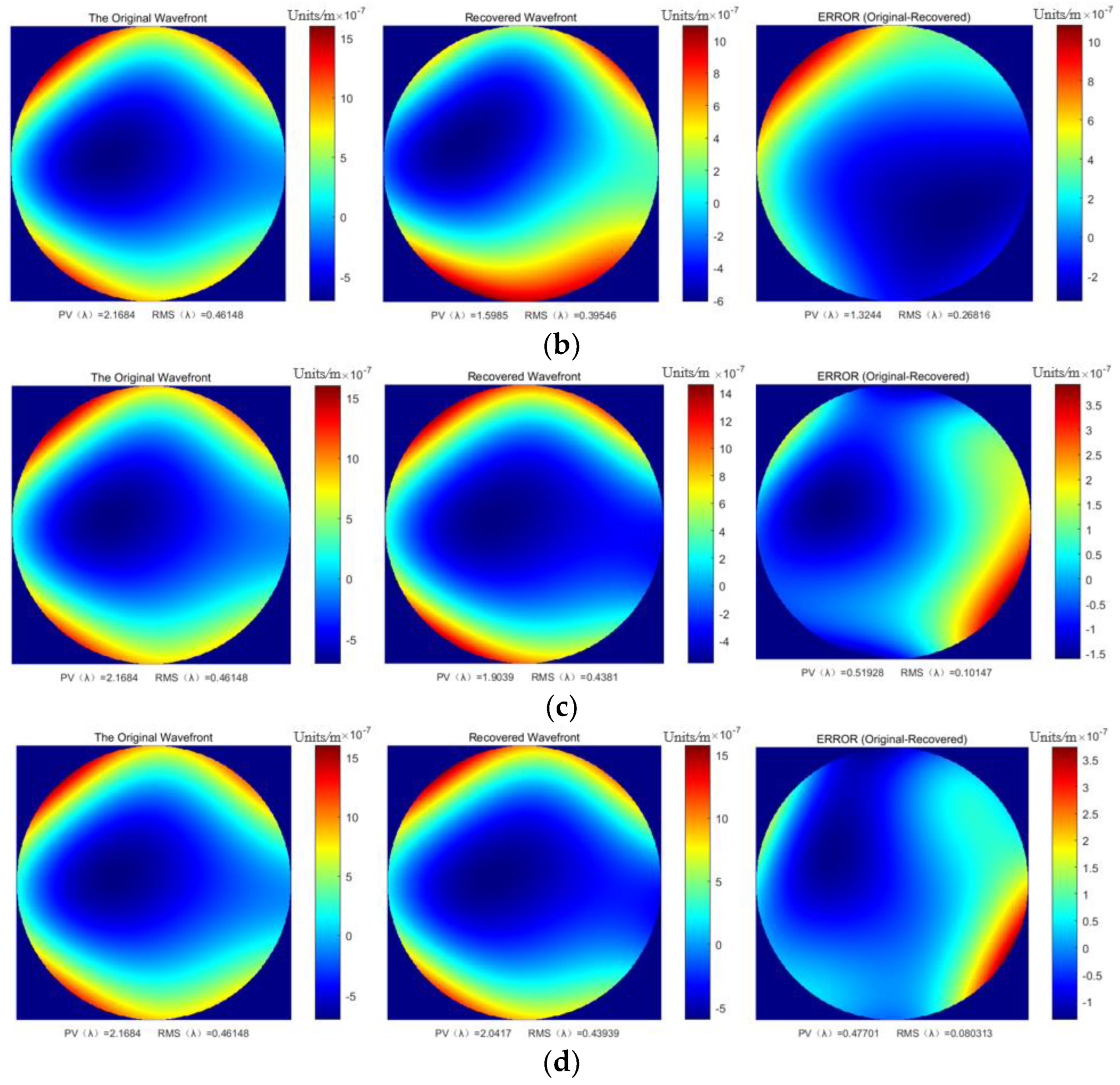
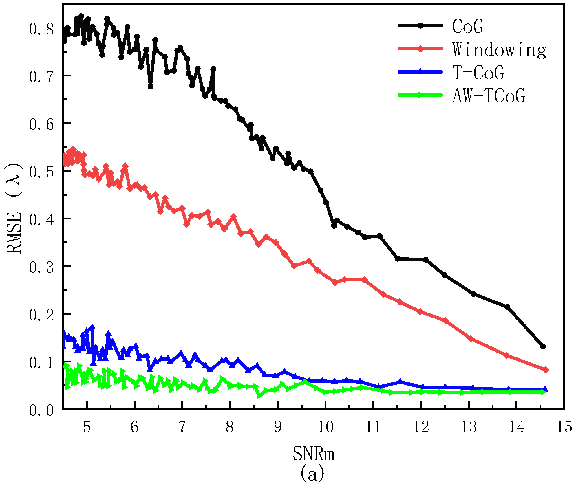
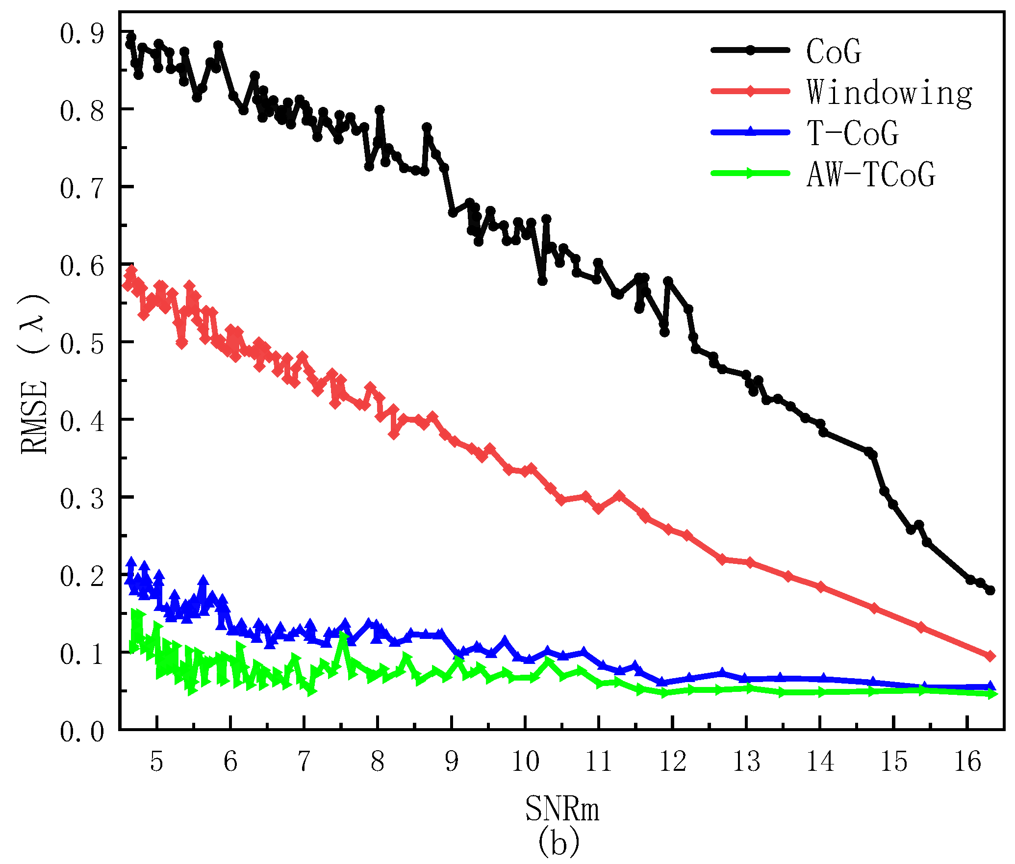
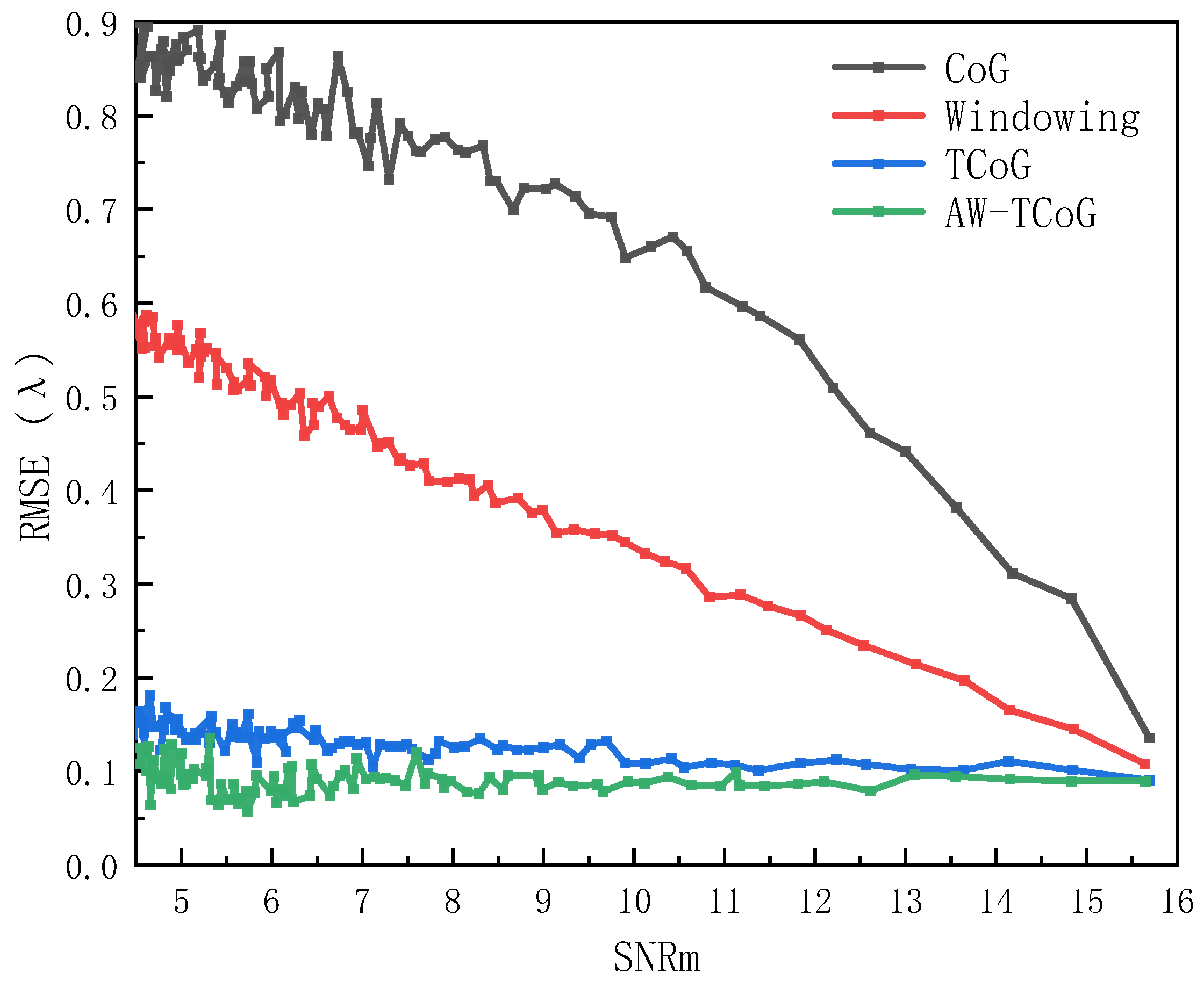
3.2. Centroid Algorithm and Wavefront Reconstruction Accuracy

The mean filtering method is used to process the image globally, and then the CoG, the T-CoG, the Windowing, and the AW-TCoG proposed in this paper are used to extract the centroid of the spot image after filtering. Among them, T-CoG removes noise by subtracting the background mean and triple standard deviation from the gray value of the spot image in the sub-aperture, and the Windowing method limits the pixel area about the centroid extraction in the sub-aperture to reduce the noise interference of the spot.
In order to fully compare the influence of different centroid localization algorithms on the accuracy of wavefront reconstruction, this paper divides the wavefront to be measured into two different situations for discussion. Generating 200 wavefront aberrations, of which 100 wavefront RMS values are small, the other 100 wavefront RMS values are large. Figure 8 shows 200 random wavefront aberrations generated according to Formula (2).
Noise is added to 200 random wavefront aberrations in the same way, and the wavefront reconstruction accuracy at different SNR levels is calculated by using the above method. Figure 9 shows the reconstruction of the same distorted wavefront using the four methods. Figure 10 shows the wavefront reconstruction accuracy curves of the four methods at different SNR levels under two kinds of wavefront RMS values.
It can be seen from Figure 10 that there is a certain relationship between the wavefront reconstruction accuracy and the RMS value of the incident wavefront. When the wavefront RMS value is relatively small, the wavefront reconstruction accuracy is relatively high. The wavefront reconstruction accuracy of the traditional centroid algorithm and the windowed preprocessing method decreases rapidly with the decrease in SNR, which also means that it is difficult to achieve effective wavefront reconstruction by using these two methods at low SNR. The threshold centroid method can maintain the wavefront reconstruction accuracy below 0.15λ when the RMS value of the initial wavefront is small, and the wavefront reconstruction accuracy reaches 0.2λ when the RMS value of the initial wavefront is large. When using the AW-TCoG proposed in this paper, the influence of noise on centroid detection is further reduced due to the windowing processing according to the actual size of the spot, so the wavefront reconstruction accuracy is effectively improved. Regardless of whether the incident wavefront RMS value is large or small, the wavefront reconstruction accuracy is basically maintained within 0.1λ at different levels of SNR.

4. Discussion

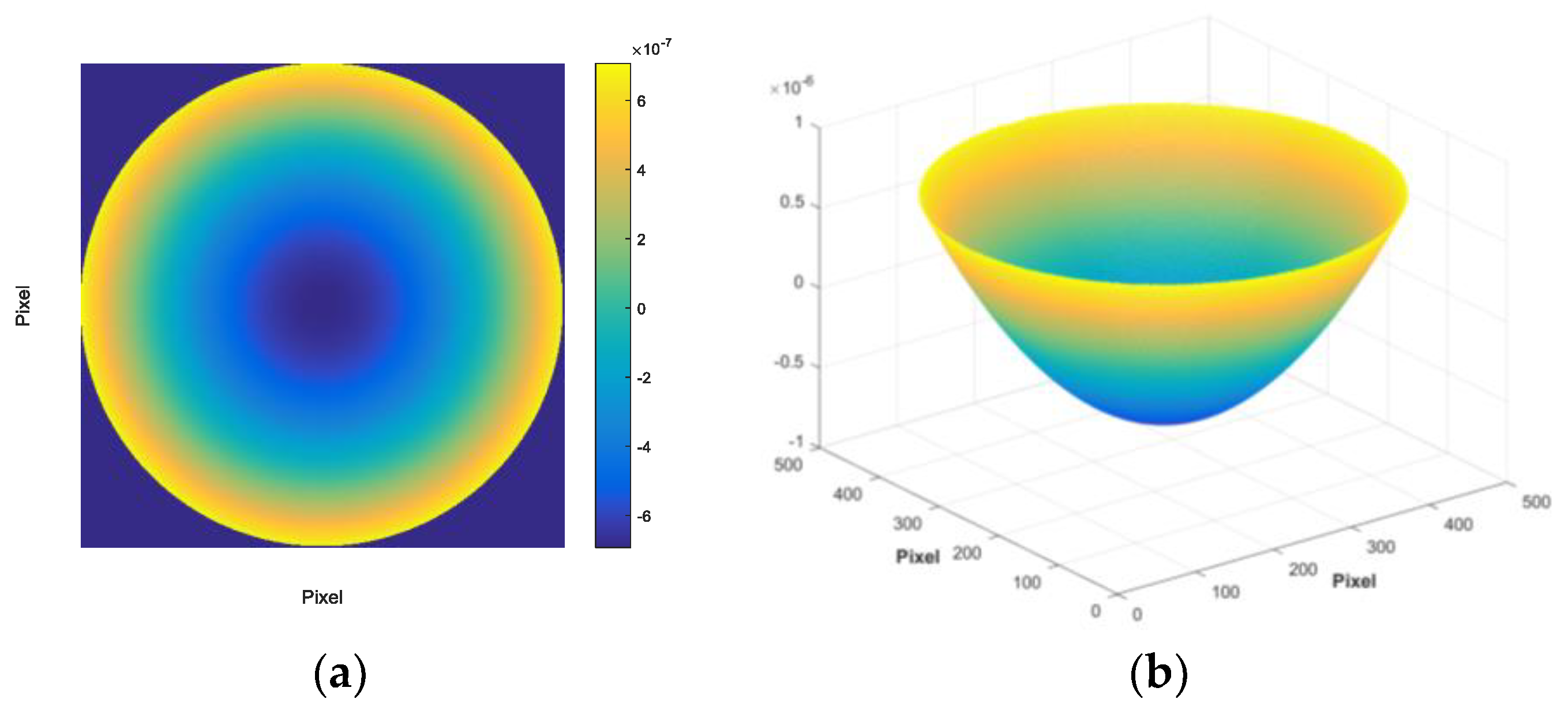
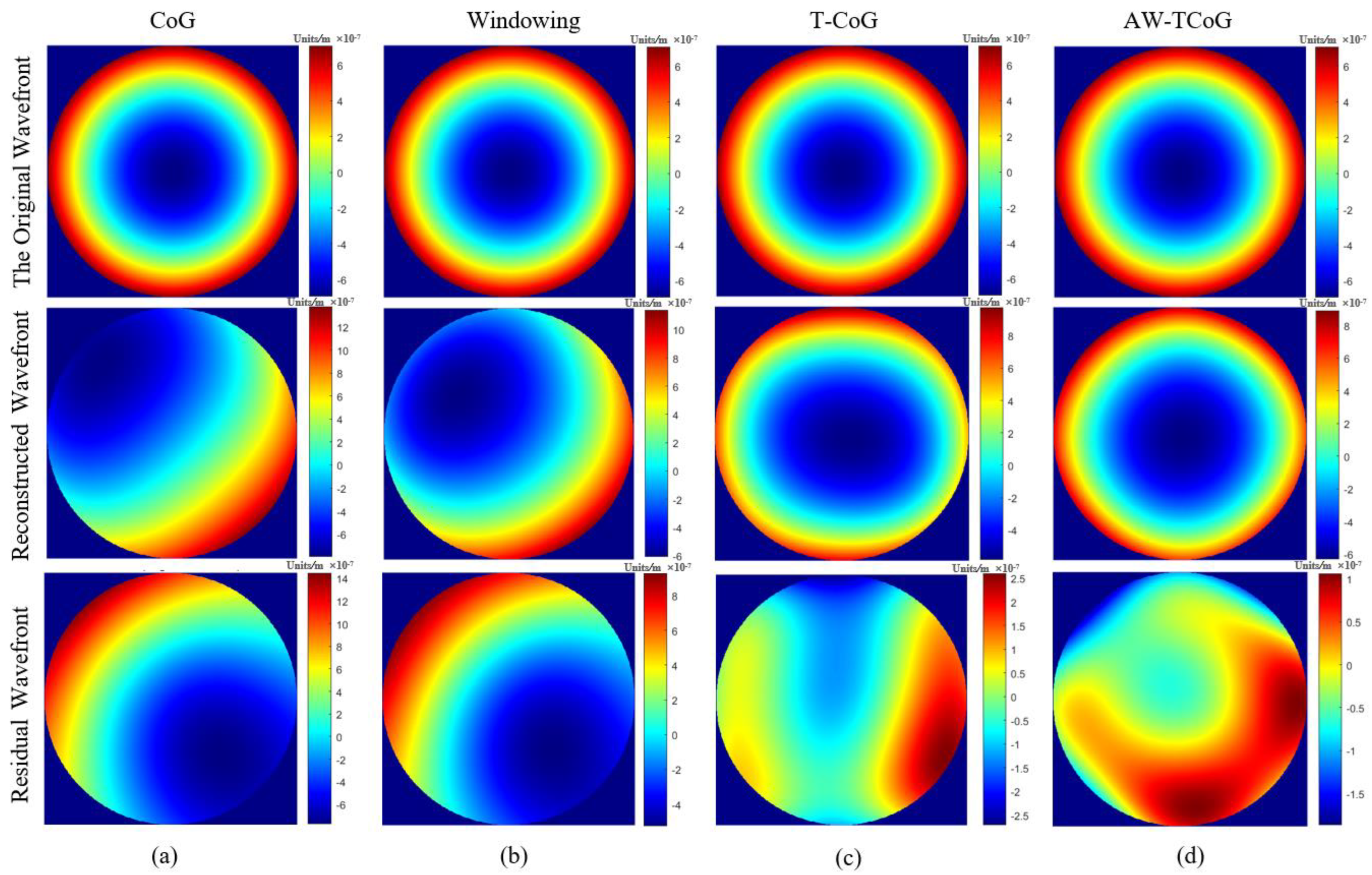
4.1. Influence of Image Processing Methods on the Defocus Aberration

The defocus was the most common aberration during our experiment, which can be expressed as:
φ = 3 ( 2 ρ 2 1 )
where ρ [ 0 , 1 ] is the defocus aberration, as shown in Figure 11. According to Formula (13), noise is added to the defocus aberration image. The CoG method, the T-CoG method, the Windowing method, and the AW-TCoG method are used to extract the centroid of the filtered image. The results are shown in Figure 12. We can obviously see that by using different methods to process the noise image of defocus aberration, the restoration accuracy gap is large. Among the four methods, the recovery accuracy of the COG method and the Windowing method is low, and the recovery accuracy of the T-COG method is significantly higher. This shows that when processing noisy images, filtering out some noise has a positive effect on improving the accuracy of image centroid detection. Because the COG method directly calculates the centroid based on the noise image, it does not reduce the influence of noise on the image to be measured, so the calculation accuracy is low. The low accuracy of the centroid calculation of the Windowing method is because only the window is added to the image to be tested. Although the influence of noise on the centroid calculation is reduced, the noise is not filtered. The T-COG method can filter out some of the noise in the image, so the accuracy of the centroid calculation is effectively improved. Based on the above three methods, the AW-TCoG method proposed in this paper not only filters the noise in the image but also combines the real-time generation window of the actual shape of the spot array to reduce the influence of residual noise, thereby improving the accuracy of the centroid calculation.

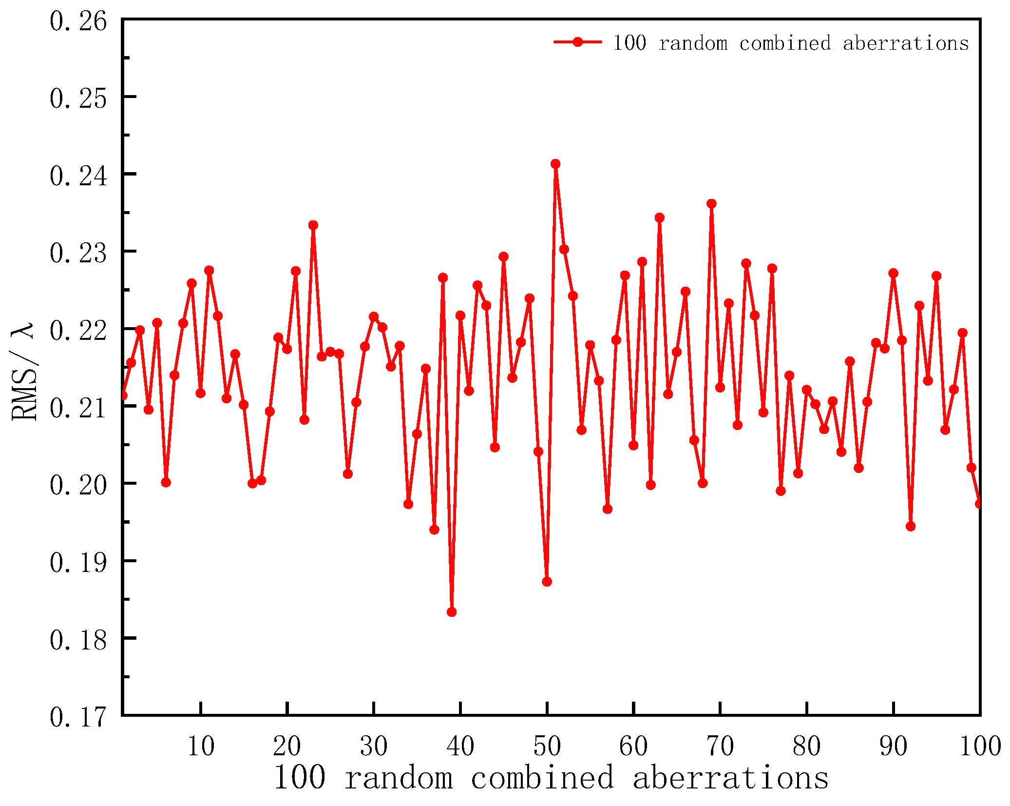
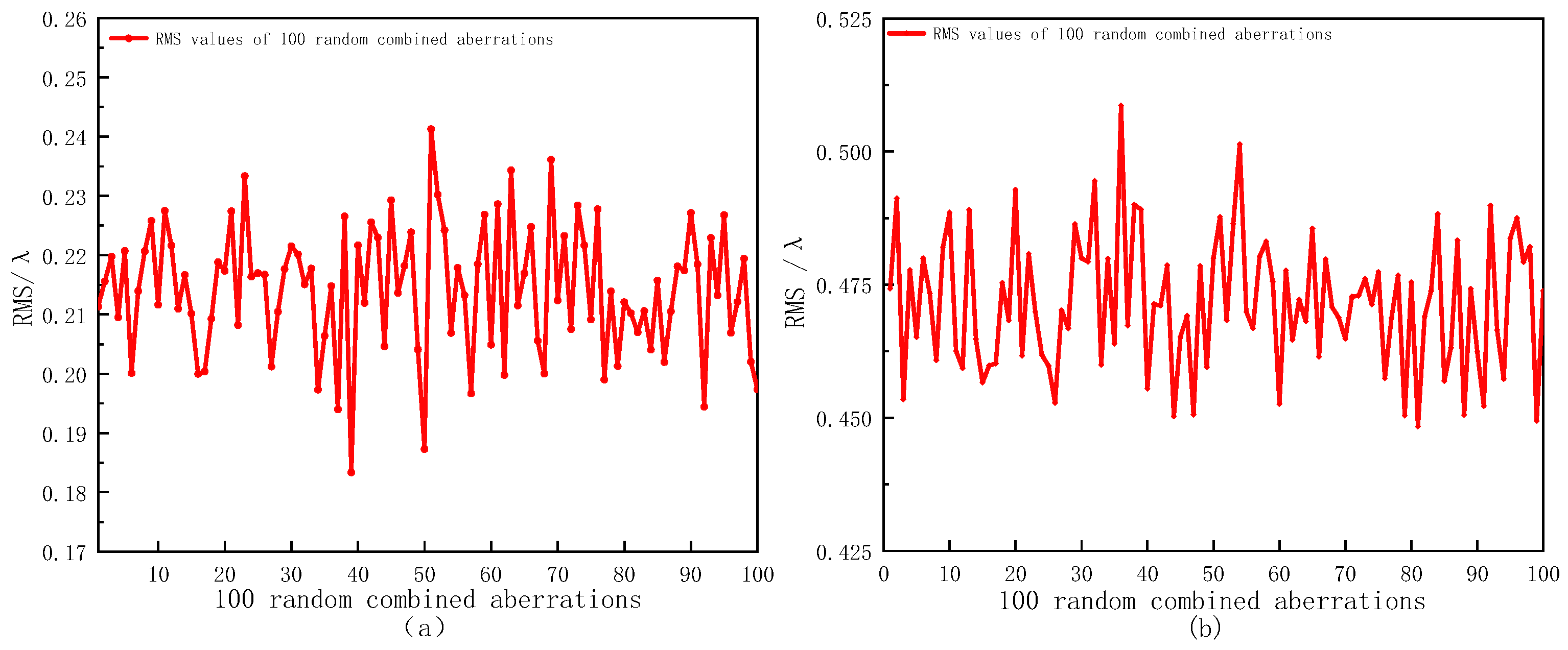
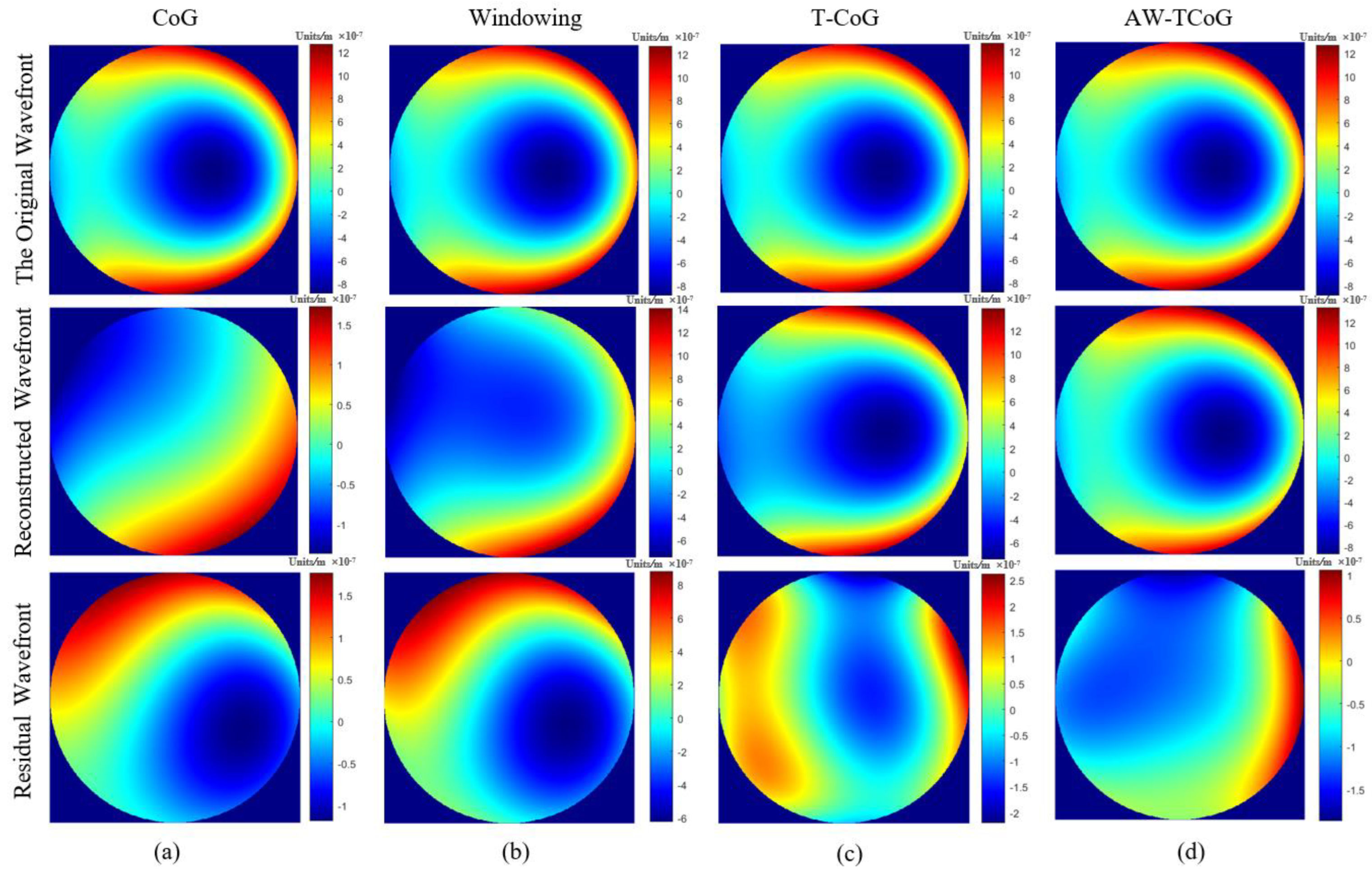
4.2. Influence of Image Processing Methods on the Mixed Aberration

In reality, the wavefront to be measured is a mixed aberration with dynamic aberration superimposed on the defocus aberration. Similarly, noise is added to the mixed aberration image according to Formula (13). The CoG method, TkCoG method, the Windowing method, and the AW-TCoG method are used to extract the centroid of the filtered image. One frame of the results is shown in Figure 13. It can be seen from the figure that the COG method and the Windowing method have low wavefront reconstruction accuracy, the T-COG method has relatively high wavefront reconstruction accuracy, and the AW-TCoG method has the best wavefront reconstruction accuracy. In addition, this paper analyzed the wavefront reconstruction accuracy of the four methods at different SNR levels in the case of mixed aberrations. The results are shown in Figure 14.
According to Figure 14, we can see that the TCoG method and the AW-TCoG method have higher reconstruction accuracy for the mixed aberration wavefront. Among them, the reconstruction accuracy of the TCoG method for the mixed aberration wavefront is kept below 0.2λ, and the wavefront reconstruction accuracy can reach 0.1λ only when the SNR is high. The reconstruction accuracy of the AW-TCoG method for the mixed aberration wavefront can be stably maintained at about 0.1λ at different SNR levels. The above results fully prove that the proposed algorithm in this paper further improved the wavefront reconstruction accuracy of different aberration wavefronts at various SNR levels compared with other classical algorithms.

5. Conclusions

In this paper, an adaptive window preprocessing algorithm based on the threshold center of gravity method is proposed, which can effectively improve the centroid detection accuracy of the spot and further improve the reconstruction accuracy of the wavefront. The influence of median filtering and mean filtering on the accuracy of wavefront reconstruction is studied. The results show that the processing effect of the spot is better, and the accuracy of wavefront reconstruction is higher when mean filtering is used. The wavefront reconstruction accuracy of CoG, Windowing, and T-CoG methods at different SNR levels under different incident wavefront RMS values is compared and analyzed. The results show that when the wavefront RMS value is relatively small, the wavefront reconstruction accuracy of the three methods is relatively high. However, the wavefront reconstruction error of the CoG method and the Windowing method increases significantly with a decrease in the image SNR. Therefore, these two methods can only meet the accuracy requirements of the system when the SNR is high. The wavefront reconstruction accuracy can be stably maintained below 0.2λ using the T-CoG method combined with mean filtering. When AW-TCoG is used, the wavefront reconstruction accuracy is kept within 0.1λ for different incident wavefront RMS values and spot images with different SNR levels, which is significantly improved compared with the threshold centroid method. In summary, the centroid localization algorithm proposed in this paper has a positive effect on the effective restoration of the wavefront under different SNR levels and promotes further improvements in wavefront reconstruction accuracy.

Author Contributions

Conceptualization, G.W.; methodology, Z.H. and Y.W.; software, G.W. and Y.L.; writing—original draft preparation, G.W., L.Q. and X.J.; writing—review and editing, G.W. and L.Q. All authors have read and agreed to the published version of the manuscript.

Funding

This research was funded by the National Natural Science Foundation of China (Grant No. 41875033).

Institutional Review Board Statement

Not applicable.

Informed Consent Statement

Not applicable.

Data Availability Statement

Data are available upon request.

Conflicts of Interest

The authors declare no conflict of interest.

References

  1. Chen, Y.; Wang, S.; Xu, Y.; Dong, Y. Simulation and Analysis of Turbulent Optical Wavefront Based on Zernike Polynomials. In Proceedings of the 2013 IEEE International Conference on Green Computing and Communications and IEEE Internet of Things and IEEE Cyber, Physical and Social Computing, Beijing, China, 20–23 August 2013; pp. 1962–1966. [Google Scholar]
  2. Chimitt, N.; Chan, S.H. Simulating anisoplanatic turbulence by sampling intermodal and spatially correlated Zernike coefficients. Opt. Eng. 2020, 59, 083101. [Google Scholar] [CrossRef]
  3. Gangyu, W.; Zaihong, H.; Laian, Q.; Xu, J.; Yi, W. Simulation Analysis of a Wavefront Reconstruction of a Large Aperture Laser Beam. Sensors 2023, 23, 623. [Google Scholar]
  4. Maiman, T.H. Stimulated Optical Radiation in Ruby. Nature 1960, 187, 493–494. [Google Scholar] [CrossRef]
  5. Hilda, F.; James, M.W. CCD noise removal in digital images. IEEE Trans. Image Process. A Publ. IEEE Signal Process. Soc. 2006, 15, 2676–2685. [Google Scholar]
  6. Feng, G.; Wang, Q.; Yang, P.; Zhang, J.; Wang, Z.; Liu, F. Diagnostic technology for temporal-spatial distribution of far-field high power laser beam profile. In Proceedings of the ICEOE 2011–2011 International Conference on Electronics and Optoelectronics, Dalian, China, 29–31 July 2011; pp. 30–33. [Google Scholar]
  7. Bernd, S.; Maik, L.; Klaus, M. Propagation of laser beams from Hartmann-Shack measurements. In Photonics North; SPIE: Bellingham, WA, USA, 2006; Volume 6343. [Google Scholar]
  8. Han, Y.N.; Hu, X.Q.; Dong, B. Iterative Extrapolation Method to Expand Dynamic Range of Shack-Hartmann Wavefront Sensors. Acta Opt. Sin. 2020, 40, 85–92. [Google Scholar]
  9. Chen, C.L.; Zhao, W.; Zhao, M.M.; Wang, S.; Zhao, C.S.; Yang, K.J. Sub-spot centroid extraction algorithm based on noise model transformation. Acta Opt. Sin. 2023, 43, 111–121. [Google Scholar]
  10. Lin, R.Z.; Yang, X.Y.; Zou, J.; Zhu, J.G.; Wu, B. Study on the center extraction precision of image photographed by CCD for large scale in spection. Transducer Microsyst. Technol. 2010, 29, 51–53. [Google Scholar]
  11. Tang, S.J.; Zhou, Z.F.; Guo, X.S.; Xiao, Y.C.; Xi’an Research Inst. of Hi-tec Hongqing Town, Xi’an 710025 China. Improved Iteration Centroid Algorithm Based on Linear CCD Light-spot Location. In Proceedings of the 2009 9th International Conference on Electronic Measurement & Instruments, Beijing, China, 16–19 August 2009; pp. 451–453. [Google Scholar]
  12. Cheng, J.; Xie, Y.; Zhou, S.; Lu, A.; Peng, X.; Liu, W. Improved Weighted Non-Local Mean Filtering Algorithm for Laser Image Speckle Suppression. Micromachines 2022, 14, 98. [Google Scholar] [CrossRef]
  13. Wang, B.; Xiang, Q. Fast Median Filter Image Processing Algorithm and Its FPGA Implementation. Front. Signal Process. 2020, 4, 88–94. [Google Scholar] [CrossRef]
  14. Li, G.P.; Chen, C.; Li, D.; Wu, L.; Zhang, B.; Yu, D.J.; Yin, W.H. Study on parameters measurement technology of high energy and high power laser. J. Appl. Opt. 2020, 41, 645–650. [Google Scholar]
  15. Guo, Y.; Zhong, L.; Min, L.; Wang, J.; Wu, Y.; Chen, K.; Wei, K.; Rao, C. Adaptive optics based on machine learning: A review. Opto-Electron. Adv. 2022, 5, 200082. [Google Scholar] [CrossRef]
  16. Himes, G.S.; Inigo, R.M. Centroid calculation using neural networks. Electron. Imaging 1992, 1, 73–87. [Google Scholar]
  17. Li, Z.; Li, X. Centroid computation for Shack-Hartmann wavefront sensor in extreme situations based on artificial neural networks. Opt. Express 2018, 26, 31675–31692. [Google Scholar] [CrossRef]
  18. Montera, D.A.; Welsh, B.M.; Roggemann, M.C.; Ruck, D.W. Use of artificial neural networks for Hartmann-sensor lenslet centroid estimation. Appl. Opt. 1996, 35, 5747–5757. [Google Scholar] [CrossRef]
  19. Wang, F.; Xie, X.; Ji, Y.F.; Duan, L.H.; Ye, X.S. Compound detector array for measuring intensity distribution of large caliber laser beam. Chin. Opt. 2012, 5, 658–662. [Google Scholar]
  20. Guan, W.L.; Tan, F.F.; Hou, Z.H. Wide Angle Array Detection Technology for High Power Density Laser. Acta Opt. Sin. 2022, 42, 159–166. [Google Scholar]
  21. Liu, M.S.; Wang, X.M.; Jing, W.B. Design of Parameters of Shack-Hartmann Wave-front Sensor for Laser-Beam Quality Meersurement. Acta Opt. Sin. 2013, 33, 302–306. [Google Scholar]
  22. Dai, F.Z.; Zheng, Y.Z.; Bu, Y.; Wang, X.Z. Zernike polynomials as a basis for modal fitting in lateral shearing interferometry: A discrete domain matrix transformation method. Appl. Opt. 2016, 55, 5884–5891. [Google Scholar] [CrossRef] [PubMed]
  23. Huang, J.; Yao, L.; Wu, S.; Wang, G. Wavefront Reconstruction of Shack-Hartmann with Under-Sampling of Sub-Apertures. Photonics 2023, 10, 65. [Google Scholar] [CrossRef]
  24. Wei, P.; Li, X.Y.; Luo, X.; Li, J.F. Design and Verification of Digital Simulation Platform for Shack-Hartmann Wavefront Sensors. Chin. J. Lasers 2021, 48, 141–150. [Google Scholar]
  25. Noll, R.J. Zernike polynomials and atmospheric turbulence. JOSA 1976, 66, 207–211. [Google Scholar] [CrossRef]
  26. Lardiere, O.; Conan, R.; Clare, R.; Bradley, C.; Hubin, N. Compared performance of different centroiding algorithms for high-pass filtered laser guide star Shack-Hartmann wavefront sensors. In Proceedings of the Conference on Adaptive Optics Systems II, Proceedings of SPIE, San Diego, CA, USA, 27 June–2 July 2010; Volume 7736. [Google Scholar]
  27. Li, X.; Li, X.; Wang, C. Optimum threshold selection method of centroid computation for Gaussian spot. In AOPC 2015: Image Processing and Analysis China; SPIE: Bellingham, WA, USA, 2015. [Google Scholar]
Figure 1. System structure and sub-aperture arrangement diagram.
Photonics 10 00799 g001
Figure 2. Binary image processing.
Photonics 10 00799 g002
Figure 3. Diagram of adaptive spot windowing threshold centroid method.
Photonics 10 00799 g003
Figure 4. Figure showing 100 random combined aberrations.
Photonics 10 00799 g004
Figure 5. Sub-aperture spot noise filtering (SNRm = 5). (a) Original image, (b) image with noise, (c) mean filtering algorithm, (d) median filtering algorithm.
Photonics 10 00799 g005
Figure 6. Sub-aperture spot noise filtering (SNRm = 12). (a) Original image, (b) image with noise, (c) mean filtering algorithm, (d) median filtering algorithm.
Photonics 10 00799 g006
Figure 7. The wavefront reconstruction accuracy under different SNRs.
Photonics 10 00799 g007
Figure 8. RMS values of 200 random combined aberrations. (a) 0.18λ < RMS < 0.25λ, (b) 0.45λ < RMS < 0.525λ.
Photonics 10 00799 g008
Figure 9. Reconstruction of the same wavefront by different methods. (a) CoG, (b) Windowing, (c) T−CoG, (d) AW−TCoG.
Photonics 10 00799 g009aPhotonics 10 00799 g009b
Figure 10. The wavefront reconstruction accuracy of different methods under different SNRs. (a) Wavefront RMS value: 0.18λ < RMS < 0.25λ, (b) Wavefront RMS value:0.45λ < RMS < 0.525λ.
Photonics 10 00799 g010aPhotonics 10 00799 g010b
Figure 11. The defocus aberration. (a) Two dimensions, (b) three dimensions.
Photonics 10 00799 g011
Figure 12. The influence of four image processing methods on the defocused aberration. (a) CoG, (b) Windowing, (c) T−CoG, (d) AW−TCoG.
Photonics 10 00799 g012
Figure 13. The influence of four image processing methods on the mixed aberration. (a) CoG, (b) Windowing, (c) T−CoG, (d) AW−TCoG.
Photonics 10 00799 g013
Figure 14. The wavefront reconstruction accuracy of different methods under different SNRs.
Photonics 10 00799 g014
Table 1. System parameters.
ParameterDescriptionParameter
Beam aperture/mm125Beam aperture/mm
Beam wavelength/nm1064Beam wavelength/nm
Lens size/mm20Lens size/mm
Lens spacing/mm5Lens spacing/mm
Duty factor0.8Duty factor
Lens focal length/mm500Lens focal length/mm
Disclaimer/Publisher’s Note: The statements, opinions and data contained in all publications are solely those of the individual author(s) and contributor(s) and not of MDPI and/or the editor(s). MDPI and/or the editor(s) disclaim responsibility for any injury to people or property resulting from any ideas, methods, instructions or products referred to in the content.

