Article

Phase Error Evaluation via Differentiation and Cross-Multiplication Demodulation in Phase-Sensitive Optical Time-Domain Reflectometry

1
NORCE Norwegian Research Centre, P.O. Box 6031, 5892 Bergen, Norway
2
Department of Electronic Systems, Norwegian University of Science and Technology (NTNU), 7034 Trondheim, Norway
*
Author to whom correspondence should be addressed.
Current address: Bundesanstalt für Materialforschung und -Prüfung, Unter den Eichen 87, 12205 Berlin, Germany.
Photonics 2023, 10(5), 514; https://doi.org/10.3390/photonics10050514
Submission received: 16 January 2023 / Revised: 17 April 2023 / Accepted: 23 April 2023 / Published: 28 April 2023
(This article belongs to the Special Issue Advances of Optical Fiber Sensors)

Abstract

:
Phase-sensitive optical time-domain reflectometry (φOTDR) is a technology for distributed vibration sensing, where vibration amplitudes are determined by recovering the phase of the backscattered light. Measurement noise induces phase errors, which degrades sensing performance. The phase errors, using a differentiation and cross-multiplication (DCM) algorithm, are investigated theoretically and experimentally in a φOTDR system based on a phase retrieval configuration consisting of an imbalanced Mach–Zehnder interferometer (IMZI) and a 3 × 3 coupler. Analysis shows that phase error is highly dependent on the AC component of the obtained signal, essentially being inversely proportional to the product of the power of the light backscattered from two locations. An analytical expression was derived to estimate the phase error and was confirmed by experiment. When applied to the same measurement data, the error is found to be slightly smaller than that obtained using in-phase/quadrature (I/Q) demodulation. The error, however, increases for longer measurement times.

1. Introduction

Phase-sensitive optical time-domain reflectometry (φOTDR) is a powerful distributed fiber sensing technique that has seen significant advances in recent years. In a φOTDR system, the interference of the Rayleigh backscattered light is acquired in time domain, and the obtained signal needs to be processed in order to retrieve the vibrational information. φOTDR sensors have the benefit of utilizing standard optical fibers and can be readily extended to long fiber lengths. They have been applied to structural health monitoring, environmental monitoring, geophysical experiments, and perimeter security surveillance [1,2,3,4,5].
Optical fibers are not perfectly uniform along their length and consist of inhomogeneities. Consequently, the refractive index varies randomly along the fiber. Thus, a small portion of the incident optical pulse is backscattered, and the light components scattered within the pulse length interfere. External stimuli change the local scattering properties of the fiber, modifying the phase delay imparted to the backscattered light and therefore also the resulting interference characteristics. Hence, environmental perturbations (temperature, strain, etc.) are retrieved from the optical amplitude or phase information. Phase-based methods are able to measure the vibration amplitude without the need for slow frequency scanning, so they are particularly suitable for distributed acoustic sensing. The optical phase can be obtained by either coherent detection or direct detection. In coherent detection, a local oscillator is mixed with the backscattered light, and its beat is detected to calculate the phase [6]. Direct detection usually exploits an interferometer to encode the phase information on to intensity variations [7,8].
Several demodulation methods have been used to retrieve phase information. In-phase/quadrature (I/Q) demodulation is a popular method that has been applied to φOTDR systems based on both direct and coherent detection [6,9]. The in-phase (I) and quadrature (Q) components are obtained from the detected signal, and the arctangent of their ratio represents the optical phase. The differentiation and cross-multiplying (DCM) algorithm is also a demodulation method that is mainly used in the direct detection scheme. The DCM algorithm has been applied to phase recovery in φOTDR systems with 2 × 2 or 3 × 3 couplers at the receiver [7,10]. Phase-generated carrier (PGC) demodulation is another method and relies upon a frequency modulation of the backscattered light. The signals of the fundamental carrier at the modulated frequency and its second harmonic carrier are measured, and the phase is recovered using I/Q demodulation or DCM [11,12]. The PGC exhibits large dynamic range and high sensitivity but requires extra hardware for the frequency modulation [13]. In general, the same phase retrieval algorithm can be applied to numerous φOTDR configurations; for example, I/Q demodulation has been applied to retrieve the optical phase for φOTDR systems based on both coherent detection schemes and the IMZI scheme. Conversely the signal from one sensing scheme can be demodulated using different methods, e.g., both the I/Q demodulation and DCM algorithm can be used to obtain the phase for the φOTDR systems based on the IMZI scheme.
The error of the retrieved phase, or the phase variance over time at a given position, is a key performance indicator for φOTDR systems and determines the minimum detectable strain. The obtained φOTDR signal trace is a random value along the fiber, depending on variables such as optical frequency, fiber properties, and ambient environment. These variables all contribute to determining the interference visibility at any given location along the fiber. The dominant noise is from the photodetector for an optimized system. As a result, the SNR and the phase error turn out to be position-dependent, and the overall performance along the fiber can only be evaluated in a statistical manner. Phase errors have been investigated for various φOTDR schemes based on I/Q demodulation [14,15,16]. In [14,15], the phase error obtained in a φOTDR system based on coherent detection was statistically investigated and its probability density function was derived. The phase error obtained for a φOTDR system based on direct detection has also been comprehensively analyzed in [16]. Previous research considers the detection noise as a constant along the fiber. A recent study demonstrated that the photodetection noise is usually proportional to the amplitude of the local signal, thus varying randomly along the fiber [17]. The previous method [16] was then modified to provide a more accurate estimation of the phase error [18]. However, to the best of our knowledge, no phase error analysis exists yet for the DCM algorithm. Such an analysis is of interest to the research community, because this phase retrieval algorithm has been widely used not only in distributed fiber sensing but also discrete sensing [19].
In this paper, the phase error obtained by the DCM algorithm is investigated theoretically and experimentally, taking as an example a φOTDR system based on an imbalanced Mach–Zehnder interferometer (IMZI) with a 3 × 3 coupler. The performance of the DCM algorithm is compared with that of I/Q demodulation. A detailed study of the latter was presented in a previous paper [16]. The performance comparison was performed by applying both methods to the same measurement data, which were collected under static conditions. The investigation showed that compared with I/Q demodulation, the DCM algorithm leads to slightly smaller phase errors, but the error becomes larger as the number of measurements increases. The increase in phase error with measurement time probably occurs because the detection noise accumulates during the multistep nature of the DCM calculation process.

2. Working Principle

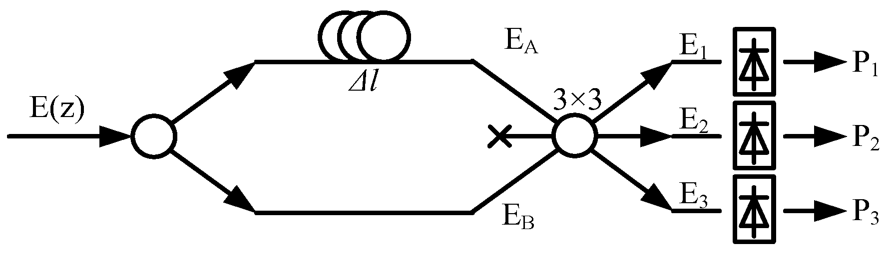
2.1. Phase Retrieval Based on IMZI Scheme
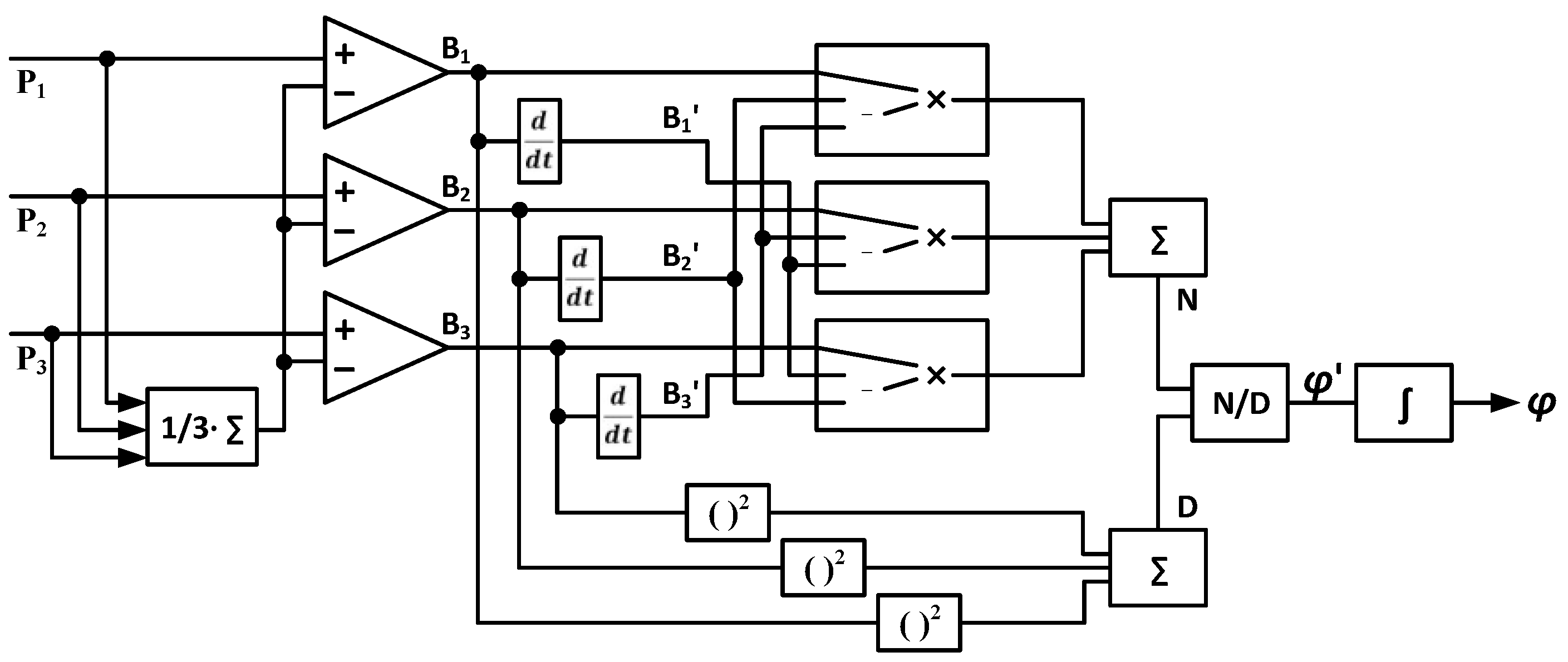
In this paper, a φOTDR system with an IMZI and a 3 × 3 coupler is used to investigate the phase error obtained by a digital DCM algorithm. For such a sensing system, the phase information can also be retrieved using the I/Q demodulation technique, making it possible to compare how the two phase recovery methods perform under the same conditions.
In the typical IMZI scheme, as shown in Figure 1, the Rayleigh backscattered light E z , t from an arbitrary position z is first evenly divided by a splitter, and one component is then delayed relative to the other. The path length difference l determines the gauge length of the sensor. The two components are then recombined at a 3 × 3 coupler. In this way, the phase difference φ z , t between positions z and z + l is compared. The outputs of the coupler at time t are expressed as
{ P 1 ( z , t ) = P D C ( z , t ) P A C ( z , t ) sin [ Δ φ ( z , t ) + 2 π / 3 ] P 2 ( z , t ) = P D C ( z , t ) P A C ( z , t ) sin [ Δ φ ( z , t ) ] P 3 ( z , t ) = P D C ( z , t ) P A C ( z , t ) sin [ Δ φ ( z , t ) 2 π / 3 ]
where P A C z , t = E z , t E z + l , t / 3 and P D C = P 1 + P 2 + P 3 / 3 represent AC and DC components of the signal, respectively, and ±2π/3 is the extra phase induced by the 3 × 3 coupler. A detailed analysis can be found in [16]. The outputs of the IMZI are received by three identical photodetectors, and the phase φ z , t can be retrieved using either the DCM algorithm or I/Q demodulation.

2.2. DCM Algorithm

The DCM algorithm is a popular method for retrieving phase information from fiber sensors in general. It has been applied to φOTDR systems with an IMZI or a Michelson interferometer [7,8]. The output of the interferometer can be written as a trigonometric function of the optical phase. The DCM algorithm is able to provide an outcome proportional to the phase by differentiating all the outputs of the interferometer and multiplying the differentiation result with other outputs.
In practice, how the DCM process is implemented varies from setup to setup and can be implemented in analogue domain using electronics, or in the digital domain. The latter case is investigated here. From Figure 2, the DCM consists of four steps. The first step is to remove the DC components from each obtained signal. The next step is differentiation and cross-multiplication. The DC-removed signals are differentiated over time, and the difference between two differentiated signals are multiplied by the third DC-removed signal. The differentiation acts essentially as a high-pass filter, which is prone to noise [9]. Then, the square of the DC-removed signals are summed, and the result is divided by the sum of the output from the second step. The outcome of the division is a function proportional to the derivative of the optical phase Δφ(z) over time. The last step is an integration over t, which retrieves the phase corresponding to a given location along the fiber.
In practice, the differentiation can be replaced by subtraction, as B i z , t = B i z , t + t B i z , t t / 2 t , where t is the time interval between two successive measurements and is determined by the pulse repetition rate. Here, the DC component is assumed to be a time-independent value to simplify the analysis. Following the workflow, as shown in Figure 2, the numerator N and the denominator D of the derivative of the phase φ z , t can be expressed as
N = 1 6 Δ t { [ 2 P 1 ( z , t ) P 2 ( z , t ) P 3 ( z , t ) ] [ P 2 ( z , t + Δ t ) P 2 ( z , t Δ t ) P 3 ( z , t + Δ t ) + P 3 ( z , t Δ t ) ] + [ 2 P 2 ( z , t ) P 1 ( z , t ) P 3 ( z , t ) ] [ P 3 ( z , t + Δ t ) P 3 ( z , t Δ t ) P 1 ( z , t + Δ t ) + P 1 ( z , t Δ t ) ] + [ 2 P 3 ( z , t ) P 1 ( z , t ) P 2 ( z , t ) ] [ P 1 ( z , t + Δ t ) P 1 ( z , t Δ t ) P 2 ( z , t + Δ t ) + P 2 ( z , t Δ t ) ] } ,
D = 2 3 [ P 1 2 ( z , t ) + P 2 2 ( z , t ) + P 3 2 ( z , t ) P 1 ( z , t ) P 2 ( z , t ) P 2 ( z , t ) P 3 ( z , t ) P 1 ( z , t ) P 3 ( z , t ) ]
Thus, the derivative of the phase can be computed as φ z , t = N / D . The optical phase is finally obtained by the integration of φ z , t as
Δ φ ( z , t ) = 1 3 0 t N D d τ = 1 3 0 t Δ φ ( z , τ ) d τ
In the digital domain, numerical integration is usually realized by the trapezoidal method. Note that the obtained phase after the integration becomes independent of t .
In the ideal case, the obtained signals P 1 , P 2 , and P 3 are constant over time at a given position when there is no external perturbation. Thus, the obtained phase remains the same value for each measurement. However, various noise sources exist in the system, causing a variation in the signal, which results in a phase error. The impact of many noise sources can be minimized by using high-performance components. For example, the light source must be highly coherent and provide small phase noise. The extinction ratio of the generated optical pulses must be high enough to suppress coherent noise [20]. For low noise, the system components should be compatible, for example, by ensuring matching fiber types throughout the system and ensuring the output intensity from any given component does not exceed the maximum input intensity of the subsequent component. The influences of noise sources can also be reduced through data processing techniques; for example, empirical mode decomposition has been used to remove the laser frequency drift [21]. Even when such methods are used, the system is not noise-free, due to noise sources such as the fundamental detection noise (thermal and shot noise). The existence of these noise sources affects both the accuracy and precision of the sensor, limiting the sensing performance.
Photodetection noise is usually believed to dominate an optimized φOTDR system. Since the photodetectors used in the IMZI scheme need to be identical, it is reasonable to assume that they possess the same noise variance σ n 2 . The noise from different detectors is assumed to be statistically independent of each other for simplicity. Moreover, the noise is considered as independent of the location along the fiber, just as in [14,15,16]. This approximation simplifies the theoretical analysis and results in a simple and straightforward expression of the phase error. The different noise contributions propagate through the workflow shown in Figure 2, leading to a phase error σ φ 2 . The variance of the phase change over time is defined as the phase error, following the previous study.
According to error propagation theory [22], the variance of the phase derivative is obtained as
σ Δ φ 2 ( z ) 3 2 Δ t 2 σ n 2 M D ( z )
where M represents the number of measurements. Detailed analysis can be found in Appendix A.
Based on Equation (5), the phase error can be expressed as (see Appendix B for more detail)
σ Δ φ 2 ( z ) = t 2 3 σ Δ φ 2 = 3 t 2 2 Δ t 2 σ n 2 M D ( z ) = 3 t 2 Δ t σ n 2 D ( z )
The equation above shows that the phase error is inversely proportional to the value of the local denominator. Inserting Equation (1) into Equation (3), the denominator can be rewritten as
D ( z ) = 3 2 P A C 2 ( z ) = 1 6 E 2 ( z ) E 2 ( z + Δ l )
Therefore, the phase error obtained by the DCM algorithm is inversely proportional to the product of the power of the light backscattered from two locations.
Equation (6) also shows that the phase error is proportional to the number of measurements ( M = t / t ). Consequently, the error obtained for 100 measurement periods is expected to be a magnitude larger than the error obtained for 10 measurement periods. In Section 4, we show that Equation (6) exaggerates the error for long-time experimental measurements, which shows the error grows relatively slowly with measurement time. This discrepancy may be caused by an oversimplification of the theory, such as ignoring the influence of temperature and laser frequency drift variations. In order to quantify and compensate for this discrepancy, a coefficient is introduced to Equation (6) that depends on the measurement time. Therefore, the phase error can be finally rewritten as
σ Δ φ 2 ( z ) = C ( M ) σ n 2 / P A C 2 ( z )
where the coefficient C M can be determined by the experimental result.

2.3. I/Q Demodulation

The phase information can also be retrieved by the I/Q demodulation method. The key is to obtain the in-phase and quadrature components based on the detected signal of the output of the IMZI. The I and Q components can be expressed as [1]
{ I ( z , t ) = P 1 ( z , t ) / 2 + P 2 ( z , t ) P 3 ( z , t ) / 2 Q ( z , t ) = 3 P 1 ( z , t ) / 2 + 3 P 3 ( z , t ) / 2
Inserting Equation (1) into Equation (9), the expressions of I and Q are essentially sin and cos functions. As a result, the optical phase Δφ(z) can then be written as
Δ φ ( z , t ) = tan 1 [ Q ( z , t ) / I ( z , t ) ]
Detailed analysis can be referred to in [9]. Note that the optical phase obtained by I/Q demodulation needs to be unwrapped. Based on the obtained phase φ , the vibrational information between position z and z + z can be determined.
As analyzed in [16], the phase error obtained by I/Q demodulation can be written as
σ Δ φ 2 ( z ) = 1.5 σ n 2 / [ I 2 ( z ) + Q 2 ( z ) ]
where the time-averaged values of I and Q are needed to calculate the phases error, and σ n 2 is determined by the photodetection process for an optimized system.
For I/Q demodulation, the denominator in (11) can be rewritten as [16]
I ( z ) 2 + Q ( z ) 2 = 9 P A C 2 / 4 = E 2 ( z ) E 2 ( z + Δ l ) / 4
The summation is also dependent on the optical power of the backscattered light. It is well known that optical power obeys exponential distribution, i.e., the probability of optical power to be a small value is much larger than for it to be a large value. Consequently, it is very likely that the product is small when the light backscattered at one position is weak, resulting in a large phase error.
Hence, as for the DCM algorithm, the error of the phase reconstructed by I/Q demodulation is also dependent on the product of the optical intensity of the Rayleigh backscattered light. The intensity of the backscattered light is a random variable and obeys the exponential distribution. Consequently, the light intensity E 2 demonstrates a stochastic profile along the fiber and can be very weak at many positions, called fading points. The AC component P A C 2 becomes very small at these points; thus, a large phase error can be expected. In addition, phase hopping of ± 2 π may occur at the fading points during the phase unwrapping process for the I/Q demodulation [18]. Consequently, the phase error at the fading points becomes even larger and can reach tens of radians [16,18].

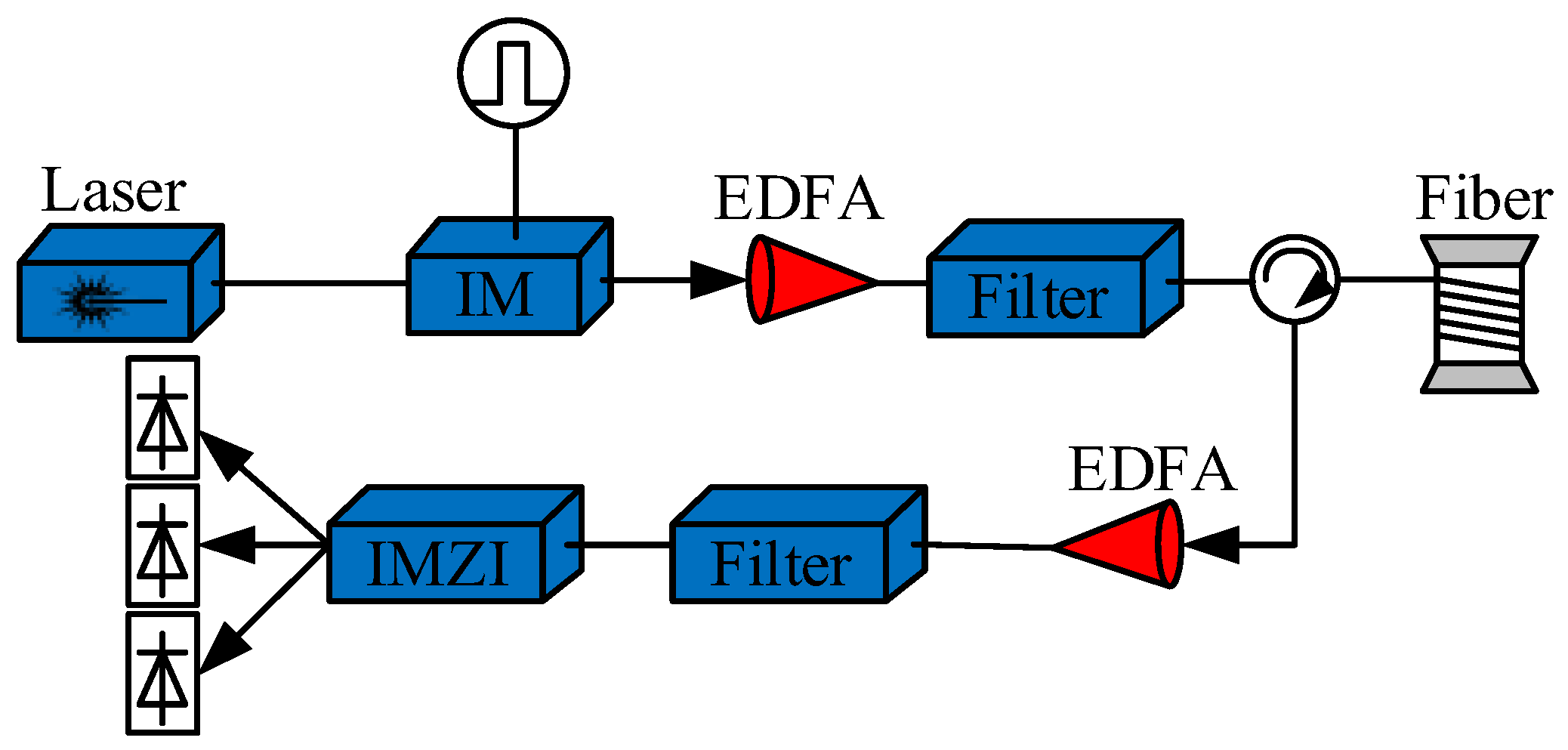
3. Experimental Setup

The theoretical analysis above was tested through an experiment. A φOTDR sensor based on the IMZI scheme was built to investigate and compare the phase errors obtained by the DCM algorithm and I/Q demodulation. The setup is shown in Figure 3. The light source is a highly coherent DFB laser working at 1550 nm. The continuous wave from the laser is converted into optical pulses with a high extinction ratio by a semiconductor optical amplifier (SOA). The generated pulses are boosted by an Erbium-doped fiber amplifier (EDFA), and the amplified spontaneous emission is suppressed by an optical filter. A variable optical attenuator (VOA) was used to adjust the optical power in such a way that sufficient backscatter intensity was achieved while avoiding modulation instability [23]. The optical pulses were coupled into a 1.44 km-long standard single-mode fiber through a circulator. The fiber length was chosen deliberately in order to have enough sampling points for statistical analysis and avoid the impact of fiber loss. The tested fiber was well isolated from environmental perturbations. The Rayleigh backscattered light was guided by the same circulator into another EDFA for amplification, before entering the IMZI scheme. The IMZI path imbalance, defining the gauge length of the sensor, was 2 m, and the output was obtained by three identical PIN photodetectors. Finally, the electrical signal was digitized and processed with the DCM algorithm and I/Q demodulation scheme using a personal computer.
The width of the optical pulse was set to 10 ns, and the 3 dB width of the backscattered light was in a frequency domain of about 60 MHz [24]. The bandwidth of the photodetectors was 125 MHz, which is larger than the 3 dB width of the spectrum, so the required spatial resolution could be achieved [24]. Additionally, the pulse repetition rate was 40 kHz. The IMZI scheme was deliberately chosen in this paper because the same setup can be used with either the DCM algorithm or I/Q demodulation phase retrieval, thus providing a fair basis for comparing these methods. In section IV, the data obtained by the φOTDR system shown in Figure 3 are first processed by DCM to confirm the analysis in section II. Following this, I/Q demodulation is applied to the same data in order to compare the obtained phase errors with the DCM results.

4. Results and Discussion

In this section, the results of the phase error obtained by the DCM algorithm are investigated theoretically and experimentally and compared with the results obtained by the I/Q demodulation. Based on the experimentally obtained signals P 1 z , t , P 2 z , t , and P 3 z , t , the optical phase φ at a given position can be retrieved using Equations (4) and (10) for DCM and I/Q demodulation, respectively. A large number of phases were obtained at the same position, since the measurement was repeated many times, and the variance value of the phase under static conditions was taken to be the experimentally determined phase error for this specific location. For the theoretical phase error, the output of each photodetector is averaged over the measurement time at every position along the fiber, and the phase error at a given position is then evaluated using the analyses presented in Section 2.2.
In order to evaluate the experimental and theoretical phase errors, 10,000 consecutive measurements of the phase profile under the same conditions were statistically investigated (M = 10,000). The whole measurement took just 0.25 s, and it was assumed that the performance of the system (e.g., laser frequency) and the environmental conditions (e.g., temperature) remained unchanged. In addition, the chosen M value was large enough for sufficient statistical convergence of the phase error, as in previous studies. Due to the system noise, the obtained phase at a given position varied during the measurements. The variance of the phases calculated by the DCM and I/Q demodulation corresponds to their respective phase errors, and the probability density function (PDF) of the error was used to compare the two phase retrieval methods.

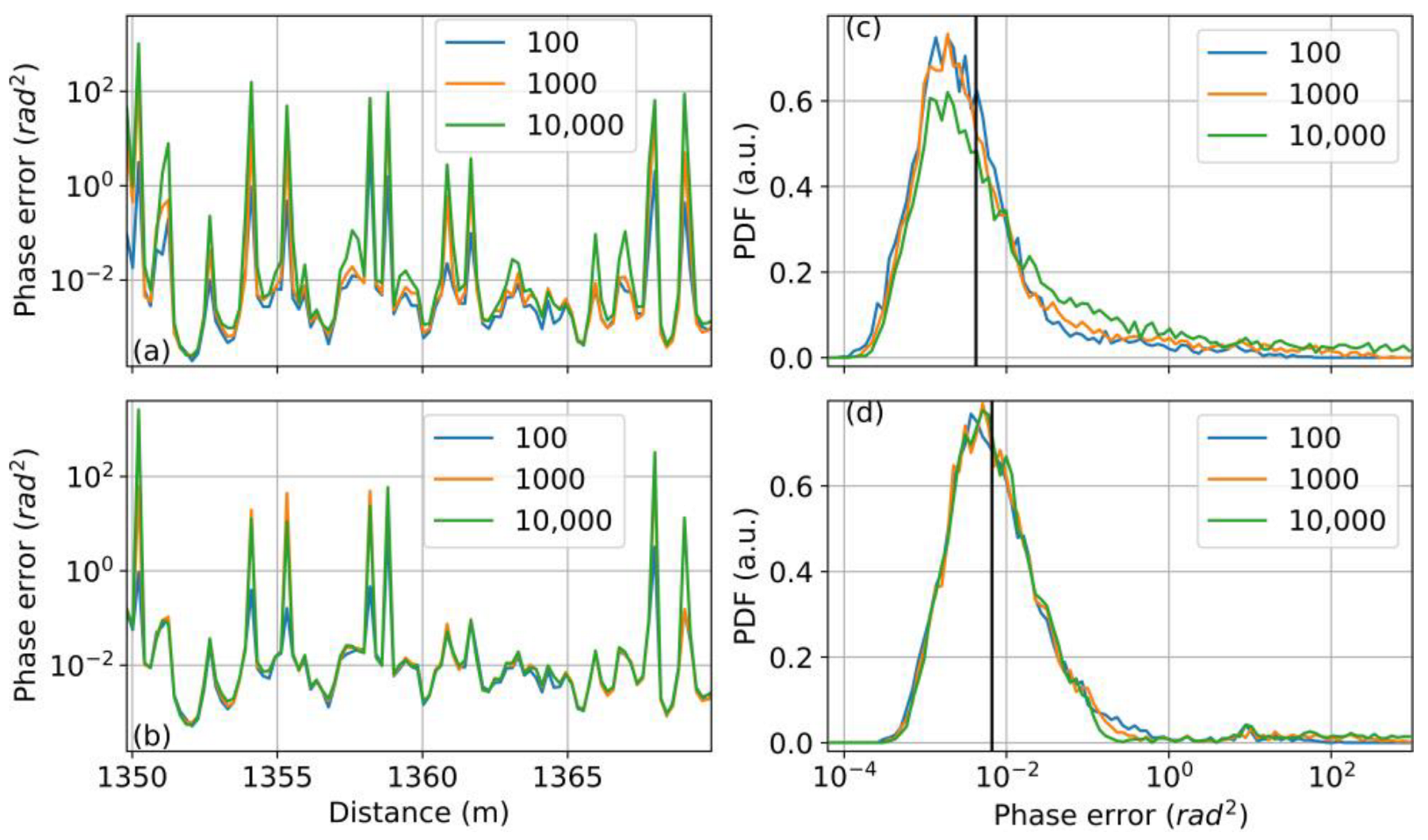
4.1. Influence of the Number of Measurements on the Phase Error

The analysis in section II B shows that the phase error obtained by the DCM algorithm is not only dependent on the AC component of the signal, i.e., the local intensity of the backscattered light, but also on the total number of measurements in time. According to Equation (6), the greater the number ( t / t ), the larger the phase error obtained. Such dependence has never been reported for the I/Q demodulation. It may be unique to the DCM, because the last step is an integration, as shown in Figure 2, that collects all the phase errors as the measurement time increases.
In order to investigate the dependence on the measurement time, the longitudinal profiles of the phase error of the DCM algorithm obtained by the first 100, 1000, and 10,000 measurements along an unperturbed fiber are depicted in Figure 4a. The error exhibits a stochastic profile along the fiber owing to the random change in the backscattered light. The phase error of the I/Q demodulation demonstrates a very similar profile, as shown in Figure 4b. It has to be pointed out that the error change over the measurement time seems to be position-dependent, particularly for the DCM algorithm. For example, the phase error remains almost the same at about 1352 m, but it changes a lot at the fading points as the measurement time increases. This may be explained by the randomness of the detected signal in the φOTDR system. According to [17], the dominant noise in the setup is proportional to the strength of the local signal and varies randomly along the fiber, just like the obtained signal. As a result, the temporal behavior of the phase error, which can be seen as the noise accumulated over the measurement time, is also position-dependent.
The profiles obtained for different numbers of measurements in time remain almost the same for the I/Q demodulation, as shown in Figure 4b, validating that the phase error obtained by this method is independent of the measurement time. However, a longer measurement leads to more phase hops, resulting in a higher error peak at the fading point. Compared with the I/Q demodulation, the phase error obtained by DCM algorithm is more dependent on the number of measurements, particularly at the fading points where the error is already relatively large. The error peaks shown in Figure 4a become higher as the number of measurements increases. As analyzed in section II B, two steps in the DCM algorithm account for this consequence: differentiation and integration. The former makes the phase retrieval method more prone to noise, and the latter makes the phase error dependent on the noise in previous measurements. It is, however, interesting to notice that the DCM algorithm results in a smaller error than the I/Q demodulation at positions with a high SNR.
Due to the stochastic profile of the phase error along the fiber, as shown in Figure 4a,b, a statistical study is necessary to quantify the nonuniformity of the error and to make a general comparison between the two phase retrieval methods.
The PDFs of the phase error obtained by the DCM algorithm and I/Q demodulation with different measurement times are plotted in Figure 4c,d, respectively. As for Figure 4a,b, the optical fiber was unperturbed during these measurements. The phase error at each location along the whole fiber contributes to the PDF. The two figures show that the PDF peak corresponding to the DCM algorithm is shifted to slightly lower values, approaching 10 3 rad2, relative to the peak for I/Q demodulation. The corresponding median (vertical line in Figure 4c) is also slightly smaller than that of the other method. This indicates that the phase error obtained by the DCM at most fiber positions are smaller than for I/Q demodulation. The PDF curve of the I/Q demodulation is almost unchanged for different numbers of measurements, as shown in Figure 4d. On the contrary, for increasing measurement times when using the DCM algorithm, the PDF decreases for phase error values < 10 2 rad2 and increases for phase errors > 10 2 rad2. This behavior reflects a general increase in phase error with measurement time.
While a comprehensive comparison between the two phase retrieval methods is beyond the scope of this paper, we make a case for the different origins for similar observed behaviors in the phase data from DCM and IQ demodulation. For the I/Q demodulation, the phase is calculated by the inverse of the tangent function, which gives a result between –π/2 and π/2. Phase unwrapping is therefore necessary to obtain the actual value. Errors may occur during this process, particularly at fading points, where the SNR is very low, which leads to a large phase error. Consequently, several high error peaks can be observed in Figure 4c. On the contrary, the DCM algorithm requires no unwrapping, but despite this, the result also exhibits high error peaks at the fading point, as shown in Figure 4a. The reason for this is believed to be due to the high influence of the noise on the denominator. This example demonstrates that similar observed behavior is caused by different factors, revealing a challenge of directly comparing the methods.
It needs to be pointed out that the obtained PDFs, as shown in Figure 4c,d, are broader than those obtained by coherent detection, as reported in [14]. The phase error obtained by coherent detection is inversely proportional to the amplitude of the backscattered light [14], whereas the error analyzed here is related to the product of the optical power at two positions. This means the phase error obtained here exhibits a higher level of longitudinal variability. Since the amplitude and power of light obey Rayleigh and exponential distributions, respectively, the product exhibits a higher level of variability along the fiber, and the phase error behaves in the same way. As a result, the PDFs shown in Figure 4 are broader than those reported in [14].

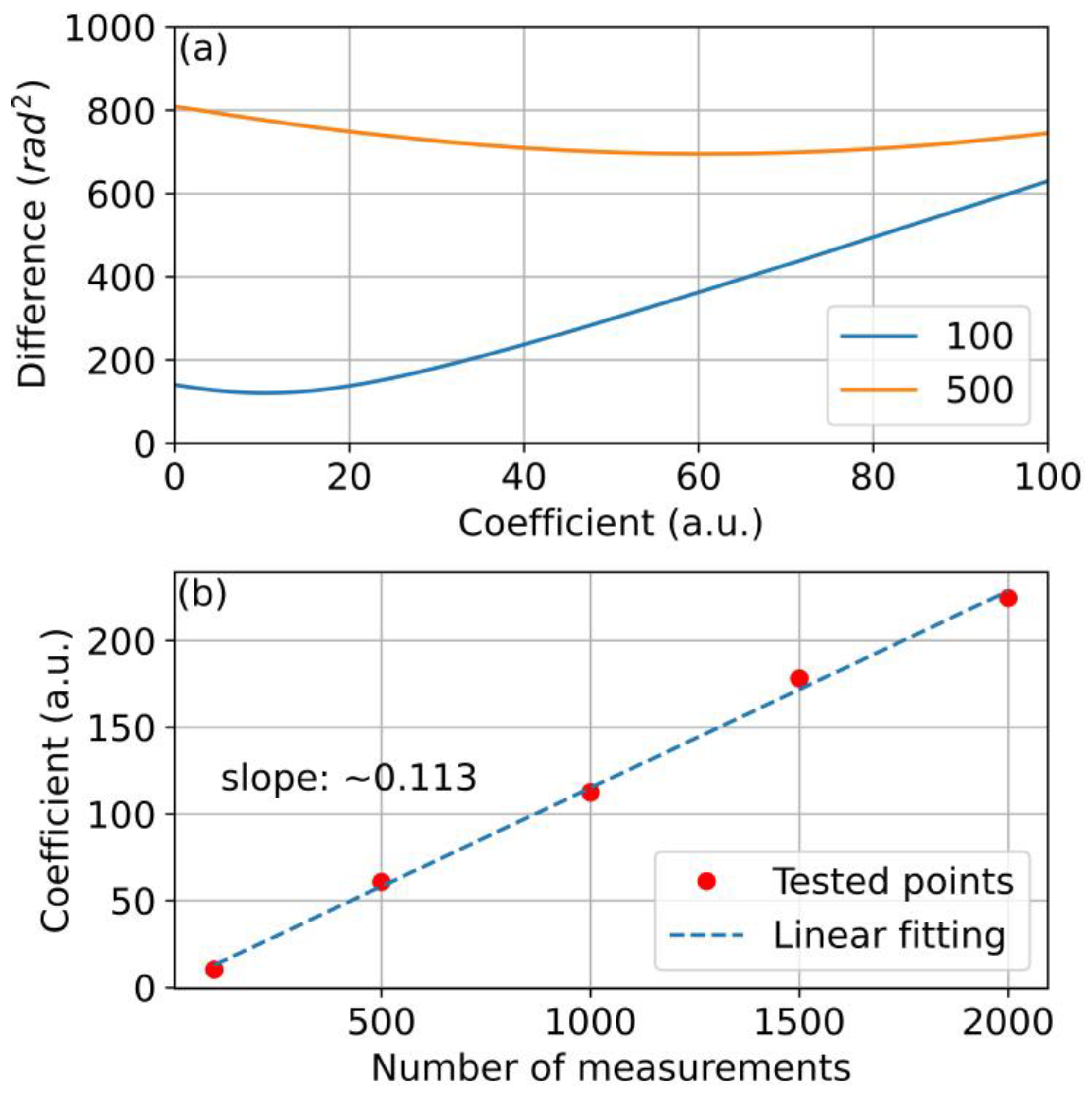
4.2. Determination of the Coefficient C

A theoretically derived expression is obtained in Section 2.2 to describe the phase error obtained by the DCM algorithm. Such a simplified expression results in a deviation from the experiment, δ , that can be quantified as
δ = j = 1 k [ σ Δ φ 2 ( z j , e x p . ) σ Δ φ 2 ( z j , t h e . ) ] 2
where k represents the total number of sampling points along the fiber, and σ φ 2 z , e x p . and σ φ 2 z , t h e . are the experimentally and theoretically obtained phase errors at position z , respectively.
The investigations presented above demonstrate that the phase error obtained by the DCM algorithm is related to the number of measurements M . The coefficient C M was introduced in section II B and can be chosen to minimize δ for any given value of M . An example is shown in Figure 5a; the δ values for M = 100 and M = 500 turn out to be a quadratic function of the coefficient. The coefficient values that minimize δ are found from the minima of these curves.
The obtained coefficients for various numbers of measurements are plotted in Figure 5b, and the coefficient reveals itself as a linear function of the number of measurements. It equals the slope of the slashed line, so the coefficient C 0.113 M . Note that the number of measurements used in Figure 5 is comparatively small in order to suppress the impact of phase hopping on the coefficient determination. The origin for the deviation between the theoretical and experimentally measured phase error relationships with M is most likely due to the theoretical analysis ignoring contributions to the phase error from other sources, such as environmental fluctuations and fluctuations in laser noise. For example, rapid random fluctuations in the environment may significantly add to the phase error for low M; however, as M increases, the measurement time may exceed the time scale of the random fluctuations, and their contribution to the overall phase error will be less significant. Such a situation would explain why the observed overall phase error increases more slowly with M compared with the theoretical prediction.

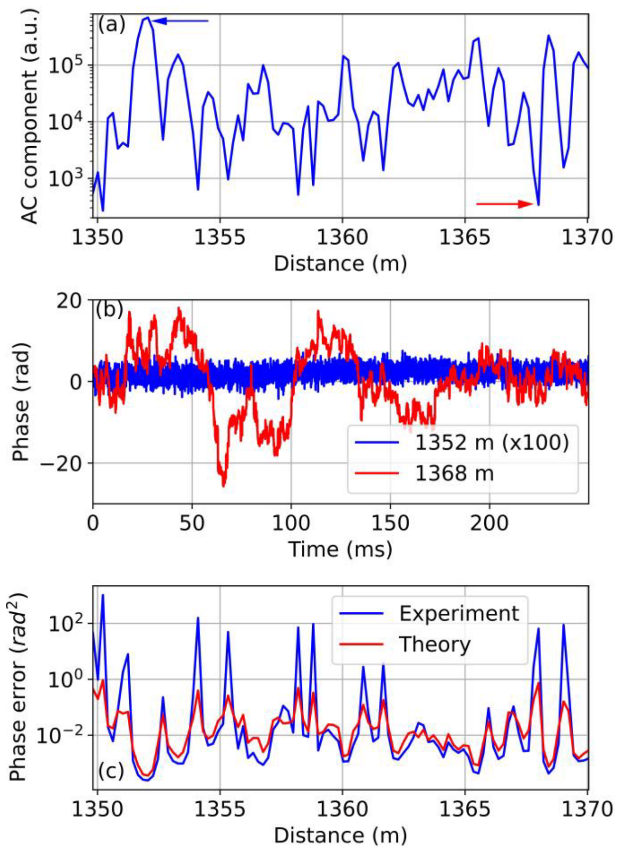
4.3. Spatial Phase Variation Characteristics under Static Conditions

As discussed in Section 2, the phase error obtained by the DCM algorithm is dependent on the AC component of the signals P A C z . Based on Equations (7) and (12), the AC component can be obtained from the I and Q component or the denominator as
P A C ( z ) = 2 / 3 D ( z ) = 2 / 3 I 2 ( z ) + Q 2 ( z )
According to the analysis in section II B, the value of P A C z is essentially determined by the optical intensities of the light backscattered at position z and z + l . At the fading point, the backscattered light is very weak; therefore, a small AC component is expected at this position. The P A C z obtained by averaging 10,000 measurements is plotted as a function of distance in Figure 6a. The randomness feature of the φOTDR signal results in a stochastic distribution of the signal difference along the fiber. As a result, the AC component varies by almost three orders of magnitude between different locations along the fiber.
Due to the random distribution of the obtained Rayleigh signal [25], the phase error exhibits a stochastic longitudinal profile along the fiber. It has been experimentally demonstrated that the error from the I/Q demodulation is related to the local I 2 + Q 2 [16]. In this section, we focus on the longitudinal distribution of the error obtained by the DCM algorithm and its relationship with the detected signals P1, P2, and P3.
The detected signals P1, P2, and P3 at a given position should be constant when the measurement is repeated under exactly the same conditions, so the obtained phase is a time-independent variable in a noise-free system. In practice, repeated measurements provide different signals due to noise σ n 2 . Consequently, the optical phase calculated by Equation (4) varies with time. Figure 6b shows the temporal change in the phase obtained at two positions that are chosen on the basis of their corresponding P A C values. Figure 6b shows that at 1352 m, where P A C is very high, the obtained phase is temporally more stable compared with at 1368 m, where P A C is low. Thus, the variance of the phase at 1352 m is smaller than that at 1368 m. The comparison presented in Figure 6b supports the theoretical analysis in Section 2.
At any given position, the temporal evolution of the obtained phase can be analyzed over the 10,000 measurements of the data series. In this way, the corresponding variance profile along the fiber can be obtained. The profile of the phase variance is presented in Figure 6c and varies randomly as expected. Based on the experimentally obtained signals, the AC component or the denominator can be calculated, and the detection noise σ n 2 can be determined as the variance of the signal. Using the obtained coefficient C M in the last section, the phase error can also be obtained theoretically by Equation (6) or Equation (8). According to Figure 6c, the theoretically obtained phase error matches well with the experimental result, validating the analysis in Section 2.2. The small deviations can be explained by the simplification in the theoretical analysis, such as considering the position dependency of the noise.

5. Conclusions

In this paper, the phase error obtained by the DCM algorithm in a φOTDR system based on the IMZI scheme with a 3 × 3 coupler is investigated. The optical phase is first analytically derived according to the phase retrieval method, and then the theoretical phase variance is obtained based on the error propagation method. The theoretical analysis presents that the phase error is dependent on the product of the optical power of the backscattered light and the number of measurements. The experimental results confirm the analysis. A statistical comparison also shows that the phase error obtained by the DCM algorithm is slightly smaller than that by I/Q demodulation. In future work, the analysis will be expanded to study the effects of a wider variety of noise sources on the phase measurement, particularly the effect of environmental fluctuations and drift in laser frequency.

Author Contributions

Conceptualization, X.L. and P.J.T.; methodology, P.J.T.; software, X.L.; validation, X.L. and P.J.T.; investigation, X.L. and P.J.T.; writing—original draft preparation, X.L. and P.J.T.; writing—review and editing, P.J.T. All authors have read and agreed to the published version of the manuscript.

Funding

The work was partially funded by the Research Council of Norway’s basic funding program.

Institutional Review Board Statement

Not applicable.

Informed Consent Statement

Not applicable.

Data Availability Statement

The data presented in this study are available on request from the corresponding author.

Conflicts of Interest

The authors declare no conflict of interest.

Appendix A

According to Equation (3), the denominator is dependent on the signal obtained by the three photodetectors, so the variance of the denominator σ D 2 is related to the noise from the detector σ n 2 = σ P 1 2 = σ P 2 2 = σ P 3 2 . In order to simplify the analysis, the outputs of the detectors are assumed as statistically independent, just as in [16]. Based on the error propagation theory [26], the variance of the denominator σ D 2 can therefore be expressed as
σ D 2 ( z ) = ( D P 1 ) 2 σ P 1 2 M + ( D P 2 ) 2 σ P 2 2 M + ( D P 3 ) 2 σ P 3 2 M   = 8 3 M σ n 2 ( P 1 2 + P 2 2 + P 3 2 P 1 P 2 P 2 P 3 P 1 P 3 ) = 4 M σ n 2 D ( z )
In order to calculate the variance, the signal P i in the equation above is replaced by its average value over the whole measurement time.
In the same way, the variance of the nominator is written as
σ N 2 ( z ) = σ n 2 4 M Δ t 2 { 2 ( P 1 P 2 ) 2 + 2 ( P 1 P 3 ) 2 + 2 ( P 2 P 3 ) 2 + [ P 1 ( t + Δ t ) P 1 ( t Δ t ) P 2 ( t + Δ t ) + P 2 ( t Δ t ) ] 2 + [ P 1 ( t + Δ t ) P 1 ( t Δ t ) P 3 ( t + Δ t ) + P 3 ( t Δ t ) ] 2 + [ P 2 ( t + Δ t ) P 2 ( t Δ t ) P 3 ( t + Δ t ) + P 3 ( t Δ t ) ] 2 } 1 M ( P 1 2 + P 2 2 + P 3 2 P 1 P 2 P 2 P 3 P 1 P 3 ) = 3 2 M σ n 2 Δ t 2 D ( z )
It is assumed that the signal remains constant, i.e., P i t + t P i t t , during the calculation to simplify the result. To obtain the variance, the average value of the signal should be used to compute (A2).
Inserting Equations (A1) and (A2) into Equation (5), according to the error propagation, the variance of the phase derivative Δφ’ is expressed as
σ Δ φ 2 ( z ) = ( N D ) 2 [ ( σ N N ) 2 + ( σ D D ) 2 2 σ N D N D ] = 3 2 M Δ t 2 σ n 2 D + 4 N 2 σ n 2 M D 3 2 N σ N D M D 3
where σ N and σ D represent the standard deviation of the numerator N and denominator D, respectively, and σ N D is the covariance of the two factors. Assuming again P i t + t P i t t , the numerator N can be approximated as 0, so the last two terms on the right-hand side of Equation (A3) can be neglected. Thus, the variance σ φ 2 can be finally expressed, as shown in Equation (5).
Note that the notations z and t are usually omitted in this appendix to obtain a short expression.

Appendix B

The variance of any variable can be obtained by subtracting the square of the mean of the variable from the mean of the square of the variable. The mean of the phase can be obtained as
E x ( Δ φ ) = E x [ 1 3 0 t Δ φ ( τ ) d τ ] = 1 3 t Δ φ ¯
where E x φ represents the expectation and Δ φ ¯ is the mean of the phase derivative.
The mean of the square of the phase can be expressed as
E x ( Δ φ 2 ) = 1 3 E x [ 0 t Δ φ ( τ ) d τ 0 t Δ φ ( μ ) d μ ] = 1 3 0 t 0 t E x [ Δ φ ( τ ) Δ φ ( μ ) ] d τ d μ = 1 3 σ Δ φ 2 0 t 0 t ρ ( τ μ ) d τ d μ + 1 3 0 t 0 t E x [ Δ φ ( τ ) ] E x [ Δ φ ( μ ) ] d τ d μ = σ Δ φ 2 3 0 t 0 t ρ ( τ μ ) d τ d μ + t 2 Δ φ ¯ 2
where ρ denotes the correlation. Thus, the variance of the phase is determined by the correlation coefficient. Assuming the obtained phases are highly correlated, then ρ 1 . As a result, the variance of the phase can be written as
σ Δ φ 2 = t 2 σ Δ φ 2 / 3
This assumption that ρ 1 holds for all (τμ) is mostly likely the source of the deviation between Equation (A6) and experimental observations, as quantified by the coefficient C(M).

References

  1. Hartog, H.A. An Introduction to Distributed Optical Fibre Sensors; CRC Press: Boca Raton, FL, USA, 2017. [Google Scholar]
  2. Filograno, L.M.; Riziotis, C.; Kandyla, M. A low-cost phase-OTDR system for structural health monitoring: Design and instrumentation. Instruments 2019, 3, 46. [Google Scholar] [CrossRef]
  3. JLindsey, J.; Martin, R.E.; Dreger, S.D.; Freifeld, B.; Cole, S.; James, R.S.; Biondi, L.B.; Ajo-Franklin, B.J. Fiber-optic network observations of earthquake wavefields. Geophys. Res. Lett. 2017, 44, 11792–11799. [Google Scholar]
  4. Fernandez-Ruiz, R.M.; Soto, A.M.; Williams, F.E.; Martin-Lopez, S.; Zhan, Z.; Gonzalez-Herraez, M.; Martins, F.H. Distributed acoustic sensing for seismic activity monitoring. APL Photonics 2020, 5, 030901. [Google Scholar] [CrossRef]
  5. Owen, A.; Duckworth, F.; Worsley, J. OptaSense: Fibre optic distributed acoustic sensing for border monitoring. In Proceedings of the 2012 European Intelligence and Security Informatics Conference IEEE, Odense, Denmark, 22–24 August 2012. [Google Scholar]
  6. Wang, Z.; Zhang, L.; Wang, S.; Xue, N.; Peng, F.; Fan, M.; Sun, W.; Qian, X.; Rao, J.; Rao, Y. Coherent Φ-OTDR based on I/Q demodulation and homodyne detection. Opt. Express 2016, 24, 853–858. [Google Scholar] [CrossRef]
  7. Posey, R.; Johnson, A.G.; Vohra, T.S. Strain sensing based on coherent Rayleigh scattering in an optical fibre. Electron. Lett. 2000, 36, 1688–1689. [Google Scholar] [CrossRef]
  8. Feng, S.; Xu, T.; Huang, J.; Yang, Y.; Ma, L.; Li, F. Sub-meter spatial resolution phase-sensitive optical time-domain reflectometry system using double interferometers. Appl. Sci. 2018, 8, 1899. [Google Scholar] [CrossRef]
  9. Masoudi, A.; Newson, P.T. High spatial resolution distributed optical fiber dynamic strain sensor with enhanced frequency and strain resolution. Opt. Lett. 2017, 42, 290–293. [Google Scholar] [CrossRef]
  10. Qian, H.; Luo, B.; He, H.; Zhang, X.; Zou, X.; Pan, W.; Yan, L. Phase demodulation based on DCM algorithm in Φ-OTDR with self-interference balance detection. IEEE Photonics Technol. Lett. 2020, 32, 473–476. [Google Scholar] [CrossRef]
  11. Fang, G.; Xu, T.; Feng, S.; Li, F. Phase-sensitive optical time domain reflectometer based on phase-generated carrier algorithm. J. Lightw. Technol. 2015, 33, 2811–2816. [Google Scholar] [CrossRef]
  12. Muanenda, Y.; Faralli, S.; Oton, J.C.; Di Pasquale, F. Dynamic phase extraction in a modulated double-pulse ϕ-OTDR sensor using a stable homodyne demodulation in direct detection. Opt. Express 2018, 26, 687–701. [Google Scholar] [CrossRef]
  13. Hou, C.; Liu, G.; Guo, S.; Tian, S.; Yuan, Y. Large dynamic range and high sensitivity PGC demodulation technique for tri-component fiber optic seismometer. IEEE Access 2020, 8, 15085–15092. [Google Scholar] [CrossRef]
  14. Gabai, H.; Eyal, A. On the sensitivity of distributed acoustic sensing. Opt. Lett. 2016, 41, 5648–5651. [Google Scholar] [CrossRef]
  15. Gabai, H.; Eyal, A. How to specify and measure sensitivity in distributed acoustic sensing (DAS)? In Proceeding of the 2017 25th Optical Fiber Sensors Conference (OFS), Jeju, Republic of Korea, 24–28 April 2017.
  16. Lu, X.; Soto, A.S.; Thomas, J.P.; Kolltveit, E. Evaluating phase errors in phase-sensitive optical time-domain reflectometry based on I/Q demodulation. J. Lightw. Technol. 2020, 38, 4133–4141. [Google Scholar] [CrossRef]
  17. Lu, X.; Krebber, K. Characterizing detection noise in phase-sensitive optical time domain reflectometry. Opt. Express 2021, 29, 18791–18806. [Google Scholar] [CrossRef]
  18. Lu, X.; Krebber, K. Phase error analysis and unwrapping error suppression in phase-sensitive optical time domain reflectometry. Opt. Express 2022, 30, 6934–6948. [Google Scholar] [CrossRef]
  19. Zhang, W.; Lu, P.; Qu, Z.; Zhang, J.; Wu, Q.; Liu, D. Passive homodyne phase demodulation technique based on LF-TIT-DCM algorithm for interferometric sensors. Sensors 2021, 21, 8257. [Google Scholar] [CrossRef]
  20. Martins, H.F.; Martin-Lopez, S.; Corredera, P.; Filograno, L.M.; Frazão, O.; González-Herráez, M. Coherent noise reduction in high visibility phase-sensitive optical time domain reflectometer for distributed sensing of ultrasonic waves. J. Lightw. Technol. 2013, 31, 3631–3637. [Google Scholar] [CrossRef]
  21. Lv, Y.; Wang, P.; Wang, Y.; Liu, X.; Bai, Q.; Li, P.; Zhang, H.; Gao, Y.; Jin, B. Eliminating phase drift for distributed optical fiber acoustic sensing system with empirical mode decomposition. Sensors 2019, 19, 5392. [Google Scholar] [CrossRef]
  22. Rouaud, M. Correlation and Independence. In Probability, Statistics and Estimation: Propagation of Uncertainties in Experimental Measurement; Lulu: Morrisville, NC, USA, 2017; pp. 47–100. [Google Scholar]
  23. Martins, F.H.; Martin-Lopez, S.; Corredera, P.; Salgado, P.; Frazão, O.; González-Herráez, M. Modulation instability-induced fading in phase-sensitive optical time-domain reflectometry. Opt. Lett. 2013, 38, 872–874. [Google Scholar] [CrossRef]
  24. Lu, X.; Soto, A.M.; Zhang, L.; Thévenaz, L. Spectral properties of the signal in phase-sensitive optical time-domain reflectometry with direct detection. J. Lightw. Technol. 2020, 38, 1513–1521. [Google Scholar] [CrossRef]
  25. Lu, X.; Thomas, J.P. Numerical modelling of φOTDR sensing using a refractive index perturbation approach. J. Lightw. Technol. 2020, 38, 974–980. [Google Scholar] [CrossRef]
  26. Ku, H.H. Notes on the use of propagation of error formulas. J. Res. Natl. Bur. Stand. 1966, 70, 263–273. [Google Scholar] [CrossRef]
Figure 1. Phase demodulation scheme based on an imbalanced Mach–Zehnder interferometer with a 3 × 3 coupler.
Photonics 10 00514 g001
Figure 2. Data processing workflow for the differentiation and cross-multiplication algorithm.
Photonics 10 00514 g002
Figure 3. Experimental setup for φOTDR system based on an imbalanced Mach–Zehnder interferometer with a 3 × 3 coupler.
Photonics 10 00514 g003
Figure 4. Comparison of the phase error between DCM algorithm and I/Q demodulation under different numbers of measurements: (a,b) longitudinal profiles of the phase errors obtained by DCM algorithm and I/Q demodulation, respectively; (c,d) probability density functions of the phase errors obtained by the two methods, respectively. The black vertical lines in (c,d) represent the median of the phase error for each phase demodulation method.
Photonics 10 00514 g004
Figure 5. Determination of the coefficient for phase error: (a) the difference δ changes as a function of different coefficient values for 100 and 500 measurements, and (b) the relationship between the coefficient and the number of measurements turns out to be linear.
Photonics 10 00514 g005
Figure 6. Longitudinal profiles corresponding to a φOTDR system based on an imbalanced Mach–Zehnder interferometer with a 3 × 3 coupler and when applying the DCM algorithm: (a) shows the AC component of the obtained signal, the blue and red arrows show the respective locations of high and low AC values, discussed in the main text, (b) compares the temporal evolution of the phases obtained at positions with a high and a low AC component, and (c) shows the experimentally and theoretically derived phase errors.
Photonics 10 00514 g006
Disclaimer/Publisher’s Note: The statements, opinions and data contained in all publications are solely those of the individual author(s) and contributor(s) and not of MDPI and/or the editor(s). MDPI and/or the editor(s) disclaim responsibility for any injury to people or property resulting from any ideas, methods, instructions or products referred to in the content.

