Article

Quantitative Detection of Microplastics in Water through Fluorescence Signal Analysis

1
Department of Industrial Engineering, University of Rome Tor Vergata, Via del Politecnico 1, 00133 Rome, Italy
2
Department of Experimental Medicine, University of Rome Tor Vergata, Via Montpellier 1, 00133 Rome, Italy
*
Authors to whom correspondence should be addressed.
Photonics 2023, 10(5), 508; https://doi.org/10.3390/photonics10050508
Submission received: 23 March 2023 / Revised: 21 April 2023 / Accepted: 26 April 2023 / Published: 27 April 2023
(This article belongs to the Special Issue Women’s Special Issue Series: Photonics)

Abstract

:
Microplastics (MPs) have recently been acknowledged as a new major and ubiquitous environmental pollutant with still unclear, yet potentially high, risks for different ecosystems and human health. Nevertheless, quantitative identification protocols rely on long and subjective visual counting necessarily performed on microscopes by well-trained operators. In this study, an automatic, fast, portable, and inexpensive method for the quantitative detection of MPs in water is proposed. The system is based on the typical optical setup of a fluorescence confocal microscope specifically adapted to automatically count dye-stained MPs in flowing liquids using a low-power laser beam. The fluorescence pulses emitted by flowing MPs are revealed and processed by a specific software using a pattern recognition algorithm to discriminate and count real fluorescence pulses out of noise fluctuations. The system was calibrated with commercial orange fluorescent 10 µm and 1 µm polystyrene microspheres, and remarkable agreement with theoretical predictions was obtained regarding different parameters. Tests were also performed with laboratory-prepared MPs dispersed in different types of real water samples. In this case, the agreement with theory was slightly worse and differences found in the quantitative results require further investigation. However, the present study demonstrated the proof of concept of a method for quick automated MP counting in water.

1. Introduction

Plastics are ubiquitous in daily life, and their increasing prevalence in the environment has become a global concern. Inadequate solid waste collection and management systems are thought to be a prominent cause of plastic pollution. The term “microplastic” was originally introduced by P.G. Ryan and C.L. Moloney [1] and then elaborated on by Richard Thompson in 2004 [2]. A recent and exhaustive definition of microplastics is “any synthetic solid particle or polymeric matrix, with regular or irregular shape and with size ranging from 1 µm to 5 mm” [3]. Microplastics (MPs) can be released into the environment directly from primary sources such as toothpaste, sunscreen, soaps, and other personal care products which intentionally contain MPs [4], or secondary sources as a result of the chemical, biological, and physical degradation of large plastic wastes [5].
The small size of MPs enables them to penetrate everywhere; they are found worldwide in terrestrial [6,7,8], aquatic [9,10,11], and atmospheric environments [12,13,14]. Their presence in Arctic and Antarctic environments [15,16] confirmed their great transfer ability. This characteristic has led to the contamination of hundreds of species of wildlife across all levels of the food chain, especially in the marine system, from small organisms such as plankton [17], mussels [18], and shrimps [19,20], to big animals such as dolphins [21], sharks [22], and whales [23]. Moreover, MPs have been found in food and bottled water. Dietary exposure to MPs is reported in salts [24], sugar [25], milk [26], bottled water [27], beer [28], and packaged meat [29]. The most characterized MP types are polyethylene (PE), polypropylene (PP), polyethylene terephthalate (PET/PETE), and polystyrene (PS). Although it has not yet been thoroughly investigated how MPs impact human health, some studies have shown the harmful effects of their chemical components and toxic contaminants adsorbed on their surface [30,31,32]. In fact, organisms that accidently ingest MPs can suffer consequences related to the transfer of contaminants from the plastics to the organism [33,34,35].
The great potential harm of MPs to living beings makes their detection an essential topic of research. Well-known detection techniques, including Raman spectroscopy and Fourier Transform Infrared Spectroscopy (FTIR), essentially provide qualitative information by identifying the polymer. Other techniques, such as pyrolysis, thermal desorption, and Gas Chromatography Mass Spectrometry (pyr-GCMS, TD-GCMS) can give information on polymer types and additives of MPs by analyzing their thermal degradation products. However, all the above-mentioned detection techniques have certain drawbacks since they require expensive and bulky instruments, are time-consuming, and require long sample-preparation procedures and skilled personnel. Above all, they are not effective in providing information on the particle number density. In fact, quantitative detection of MPs is often performed by visual inspection through a microscope, which was shown to be error-prone since it can lead to overestimation or underestimation and often requires well-trained operators. On the other hand, without cost-effective, reliable, and automatic methods for identifying and measuring MPs, we cannot fully monitor the plastic pollution in water on a vast scale.
In this regard, optical sensors could give quantitative results on the samples through the automatic analysis of the digital signal, identifying particle size, morphology, and chemical type of MPs. Several studies have reported the use of optical sensors for microplastic detection in water. Asamoah et al. [36] used a portable prototype optical sensor for the detection of transparent polyethylene terephthalate (PET) and translucent low-density polyethylene (LDPE) in fresh water based on specular light reflection signals and transmitted interference patterns. Iri et al. [37] used a low-cost optical system to detect the Raman scattering intensity of MPs in water. Nicolai et al. [38] provided a quantitative measurement of MPs in water and sludge samples based on real-time analysis of emitted fluorescence signals. However, these methods can only detect samples in a certain volume in batch mode, instead of continuous detection. Analysis of large water volumes is required, for example, to monitor clear water where the expected concentration is as low as a few particles per milliliter. This condition is met by drinking water and surface water, as well as by water for swimming pools, fish farming, and hydroponics. By combining a fluid-dynamic device and an optical sensor, the limitation of volume can be overcome [39,40].
For the detection by optical sensors with higher sensitivity and accuracy, the plastic particles must be stained with fluorescent dyes that are adsorbed on the surface and make plastic fluorescent under light excitation. The plastic particles thus become more visible and easily countable. Nile Red (9-diethylamino-5H-benzo[a]phenoxazine-5-one) is proven to be one of the most effective lipophilic solvatochromic dyes both in terms of adsorption efficiency and emitted fluorescence [41,42,43]. Nile Red (NR) can efficiently bind to plastic and emit fluorescence in a range of colors from yellow to deep red depending on the surface hydrophobicity of the plastic and the polarity of the solvents [44]. These spectral characteristics could allow classification of MPs on the basis of their polarity or even evaluate any changes that can occur over time due to oxidation of the plastics’ surface [41,45,46].
In this paper, we propose a fast, efficient, inexpensive, and portable method for quantitative detection of MPs in water based on analysis of fluorescence emissions. In the present approach, NR-stained plastic particles are forced to pass through a small detection volume where a laser beam excites the fluorescence emission that is collected and revealed by a photodetector. The electrical signal is then converted to digital and processed by a specific software, which discriminates fluorescence pulses coming from MPs out of the noise due to light scattering and other contaminants. This method might, in principle, allow a direct, quantitative detection of MPs in a continuous flow of reasonably clear water. The portability of this prototype makes it suitable for in situ microplastic analysis in rivers, lakes, ponds, water purification systems, and waterworks.

2. Materials and Methods

2.1. Experimental Setup

Figure 1 shows a schematic diagram of the present method, which was derived from a previous instrument for the detection of bacteria based on a moving sample and a different optical scheme [47,48,49]. The present method essentially included a fluorescence confocal microscope setup specifically adapted to detect labeled plastic MPs in flowing liquids. The optical setup was implemented on an optical breadboard with dimensions of 30 × 45 cm2. The liquid sample was contained in a syringe that was activated by a motor-controlled injection system (Nicogen 3546, Rome, Italy). The liquid was thus pushed by the syringe and forced to flow through a glass tube with a capillary constriction (Hilgenberg GmbH No. 4019119, Malsfeld, Germany) where the excitation of fluorescence occurred. The capillary constriction had an inner diameter of Φ = 200 μm and a length of 15 mm so as to ensure laminar flow at the excitation point up to the maximum flow rate under consideration (100 mL/h). Excitation light was generated by a 520 nm laser diode with an optical cw output power of 4.5 mW (CPS11K-EC, Thorlabs, Milan, Italy); the laser beam was reflected by a dichroic mirror into the same optical path as the fluorescence collection and then focused using a convex lens onto the capillary constriction, where the MPs were dragged by the liquid flow.
The laser light crossed the capillary and produced a cylindrical excitation volume inside the flowing liquid perpendicular to flow direction. The cross section (base) of the excitation cylinder had approximately an elliptical shape, with the longest axis perpendicular to the direction of the capillary constriction. The dimensions of this laser spot could be varied from 17 × 34 μm2 to 58 × 221 μm2 by using a two-lens collimator on the laser path (see Figure 1) and were determined using the knife edge method [50]. This enabled excitation of MPs within different portions (cross sections) of the liquid perpendicular to flow direction. The MPs that crossed the excitation volume emitted fluorescence pulses since they traveled across a limited excitation volume with a certain speed. For this reason, the effective excitation was limited in time and the fluorescence was pulsed even under a continuous light source. Fluorescence was in the orange/red spectral region due to the NR characteristics (see Supplementary Information). Fluorescence was collected by the same lens that focused the excitation laser and was sent to a photomultiplier (PMT, H10721-110 Hamamatsu, Milan, Italy) for revelation. In order to remove scattered laser light, fluorescence was spectrally filtered by the dichroic mirror and by an additional long-pass filter (FEL0550, Thorlabs, Milan, Italy) put in front of the PMT. A lens/pinhole combination spatially filtered fluorescence and improved the rejection ratio, while neutral density filters were used when necessary to reduce the incident laser power. The fluorescence pulses were transformed into time-depending electrical signals by the PMT, digitally converted with a 40 kHz sample rate by an analogue-to-digital converter (ADC), and input to a PC for software processing.
A specific pattern recognition algorithm was utilized to discriminate and count real fluorescence pulses out of noise fluctuations due to residual dye and spurious compounds in the water sample. Pulse counts were accumulated over a specific time period (typically 60 s) and the statistical distribution of the pulse time duration was provided at the end of each run.
All the measurements were compared with visual observations and particle number counts performed with a Nikon 330692 fluorescence microscope (Nikon, Tokyo, Japan) with 10× objective magnification both using a counting chamber (FUCHS-ROSENTHAL 0.0625 mm2, Laboroptik Ltd., Lancing, UK) and particle dispersion drops on microscope glass slides. Pictures were taken using the camera of a commercial smartphone.

2.2. Instrument Calibration with Commercial Fluorescent MPs

The instrument was calibrated using two commercial fluorescent particles, 10-µm polystyrene microspheres (Thermo Fisher scientific, Waltham, MA, USA) with a known concentration of particles in water (3.6 × 10⁶ beads/mL), and 1-µm carboxylate-modified polystyrene fluorescent microsphere (Thermo Fisher Invitrogen F8819, Waltham, MA, USA) with an unknown concentration. Both had fluorescent emission in the orange/red range. Firstly, 1-µm carboxylate-modified polystyrene microspheres (CMPS) were used for general instrument testing and adjustment. Then, 10-µm orange-fluorescent polystyrene microspheres (OFPS) with a known concentration were applied to check the particle number experimental counts using serial dilutions of the original OFPS water dispersion. Every test started with a blank run using only deionized (DI) water after cleaning the liquid path with ethanol and DI water. Typically, samples were pumped into the detection volume with a flow rate of 10 mL/h and data were acquired for 60 s; five tests for each concentration were carried out after letting the flow stabilize for one minute. The experimental particle number counts were compared with microscope counting. The dependence by flow rate was also studied, with flow rates of 50 mL/h and 100 mL/h with 10-µm OFPS.

2.3. Staining and Detection of Real MPs in Real Water Samples

To obtain a fluorescence signal from non-fluorescent materials, real plastic particles were stained with Nile Red (NR) dye. All the staining approaches reported in the literature differ in terms of Nile Red concentration, solvent, and staining procedure [40], but most protocols agree in the use of acetone as the dissolving solvent [46,51,52,53]. In the present study, acetone and NR dye were both purchased from Sigma-Aldrich (Milan, Italy) and used as received. NR stock solution was prepared in acetone with a concentration of 1 mg/mL.
Real MP samples were prepared using PS objects in order to use the same plastic material as the one used for calibration. Approximately 0.1 g of a PS single-use cup was cut and cleaned with distilled water before use. The plastic piece was ground with sandpaper, the powder was transferred to a 40 mL glass bottle with DI water and carefully dispersed through 30 min stirring. After that, a Whatman Grade 1 paper filter with a pore size of 40 μm (Sigma-Aldrich, Milan, Italy) was used to filter the MP dispersion and put an upper limit to the size range. Previously prepared 1 mg/mL NR stock solution in acetone was added to the PS MP solution to reach the final concentration. Two values of NR final concentration were tested: 5 mg/L and 0.1 mg/L. The MPs–dye solution was then stirred for 30 min in a dark environment. The staining result was checked with fluorescence microscope.
Three real water samples collected from different sites in the university, i.e., tap water from two different buildings and drinking water from a plumbed-in water dispenser, were spiked with the stained PS MPs–dye solution in the ratio 1:9 after filtration with the same 40 µm paper filter. In addition, the following different procedure was applied: real water samples were filtered through a 0.7 µm glass microfiber filter in order to reduce possible MPs originally present in the samples, then spiked with PS MPs and stained with NR at the final concentration of 0.1 mg/L [54]. Counts recorded with these samples are defined as positive control (water + MPs + NR). We also stained the same water samples without spiking with microplastics to record what are defined as negative control (water + NR). The samples were then injected into the capillary with a flow rate of 10 mL/h for 60 s; five tests were taken for each sample, including the blank water samples, after flow stabilization, as described in Section 2.2 for commercial OFPS microspheres.

3. Results and Discussion

3.1. Instrument Calibration

Figure 2a shows a microscopic observation of the 10 µm OFPS microspheres that were used, along with the 1 µm ones, for calibration. Figure 2b displays the typical time-dependent electrical signal produced by 10 µm OFPS microspheres flowing through the capillary at a constant flow rate of 10 mL/h and with a laser spot of 58 × 221 μm2. Light pulses of different intensity (height) and time duration τ can easily be observed. In Figure 2c, two representative pulses are reported on a larger time scale to show the different intensity and duration, together with the matching to Gaussian patterns (red lines) carried out by the PC software. The difference in intensity is reasonably due to particles crossing the excitation volume at different positions, thus experiencing different light excitation intensity due to the approximate laser Gaussian profile. On the other hand, the differences in pulse duration are more significant since they reflect the fact that the particles cross the excitation volume with different speeds according to the parabolic velocity profile of the cylindrical threads associated with laminar pressure-driven flow in circular tubes, as already observed by Poiseuille in the 18th century [55]. The highest velocity is in the middle of capillary while the flow is very slow near the wall. On the first approximation, one could consider pulse duration τ = x/v, where x is the path length that the particles travel inside the excitation volume (equal to the dimension of the laser spot along the flow) and v is the particle speed. Therefore, if the excitation volume encompasses the whole capillary section, as in this case, different pulse durations are expected as a consequence of different residence times of the single particles in the excitation volume. It should be noted that, in this case, the matching to a Gaussian pattern performed by software is obviously overdone and unnecessary to the simple purpose of pulse counting. However, it will be crucial when applied to real MPs in real water (see below), where background and noise can be much higher than in laboratory-prepared test samples. In addition, it enables recording and investigating the experimental distribution of pulse duration, as shown in Figure 2d. The pulse duration shows a peculiar asymmetric distribution with the mode of maximum count at τ M = 420   μ s and the mean at τ = 660 μs. The latter corresponds to v = 0.086 m/s, which is in excellent agreement with the value v = 0.088 m/s that can be calculated from the average flow rate (10 mL/h) and the geometry of the capillary. However, the real situation is more complex in that the pulse duration distribution should be derived from the statistical distribution of particle speed according to the parabolic velocity profile of liquid laminar flow. Moreover, it must be taken into account the fact that the particles are counted proportionally to their speed since, in a certain measurement time interval (typically 60 s), the faster cylindrical threads drag more particles in the excitation volume in comparison with the slower ones. In this context, a simple model developed within the laminar flow hypothesis (see Supplementary Materials) fits experimental data quite well (continuous curve in Figure 2d) except for the short-duration side of the statistical distribution. In fact, the experimental distribution smears below the minimum pulse duration predicted by theory; this could be explained with the velocity of some microspheres exceeding the maximum value allowed to laminar pressure-driven flow in circular tubes.

3.2. Linearity

Pulse counting measurements were performed at different particle number concentrations by performing serial dilution of the original sample and using a flow rate of 10 mL/h. In Figure 3, the experimental counts as a function of dilution (red squares) are compared with the values predicted according to laminar flow and the real particle concentration (black squares). Experimental data show a remarkable agreement with the predicted values and, consequently, an excellent linearity over more than two orders of magnitude range of concentration.
Similar results were obtained by increasing the flow rate to 50 mL/h and 100 mL/h (see Figure S1 in Supplementary Information). These findings demonstrate that the present method can really and effectively count all the plastic microbeads contained in the analyzed volume. A further verification comes from the fact that the number of counts at a specific concentration increases linearly with the flow rate, as reported in Figure 4a, since the analyzed volume scales consequently. Interestingly, the distribution of pulse duration also changes accordingly, in that the higher flow rates make the distribution shift towards shorter pulse durations (Figure 4b) since the particles take less time to travel across the excitation volume.

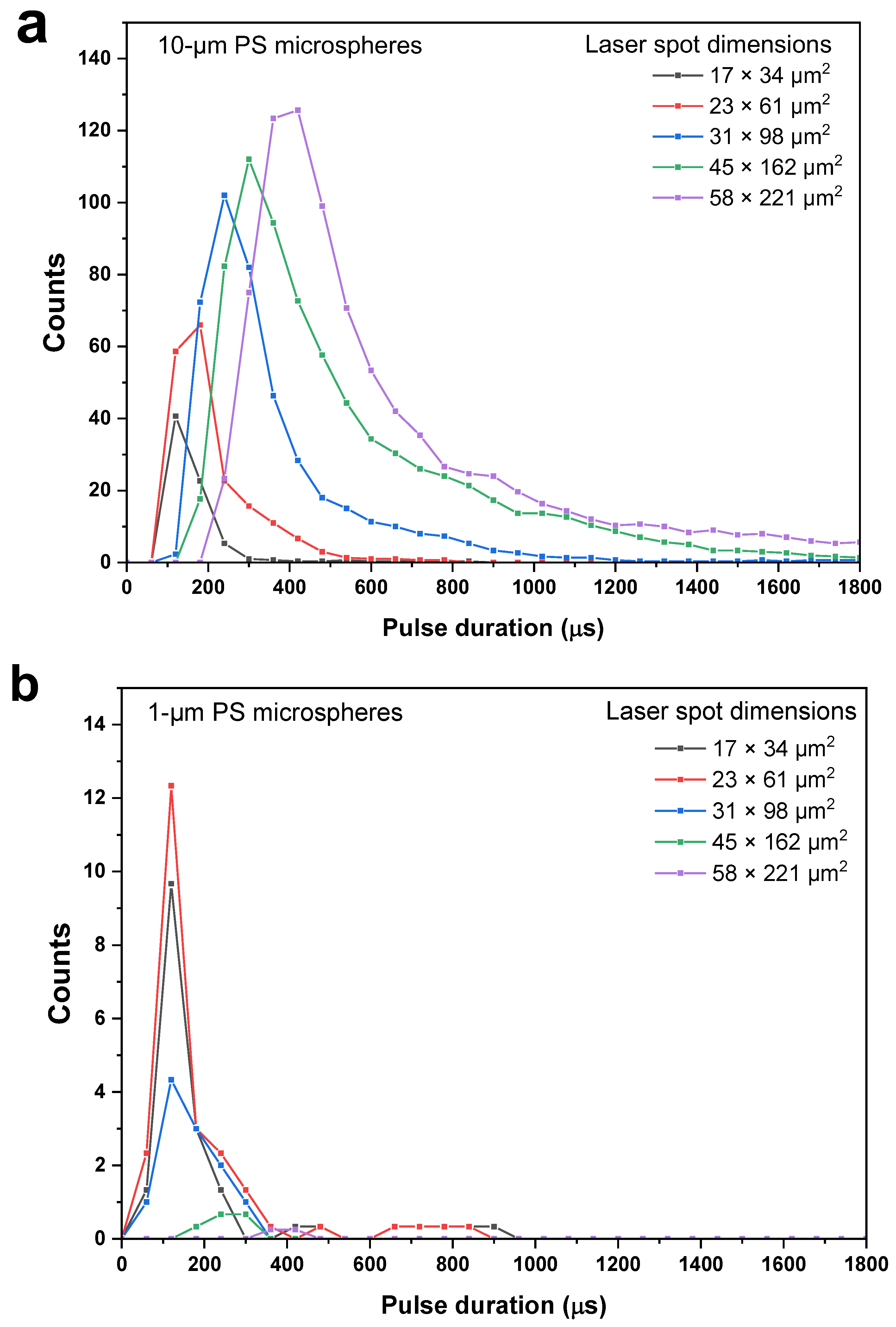
3.3. Influence of Laser Spot Dimensions

The distribution of pulse duration also changes with the dimensions of the laser beam, as reported in Figure 5. Specifically, when the excitation volume is reduced to a small portion in the center of the capillary, the distribution becomes narrower and shifts to lower transit times since only the microspheres in the faster cylindrical liquid threads closer to the capillary axis are excited and, simultaneously, the length crossed by particles becomes shorter.
In order to check the capability of the present method to discriminate the size of MP particles, the laser spot dimensions were reduced from 58 × 221 μm2 to 17 × 34 μm2 and calibration measurements were performed in the same conditions of flow rate with both 10 µm and 1 µm microbeads. As shown in Figure 5, the respective pulse duration distributions were quite different for every value of the laser spot size. In fact, when the particles are not point-like in comparison with the laser spot size, i.e., with the 10 µm beads, the effective average transit time increases due to simple geometrical considerations, and this demonstrates that our system can, in principle, distinguish between different dimensions. However, we also observed a significant drop of total counts with 1 µm spheres when the spot dimensions increased. This was likely due to the fluorescence pulses being too low to be detected when the excitation intensity decreased, and it requires further investigation, e.g., by using a more powerful laser.

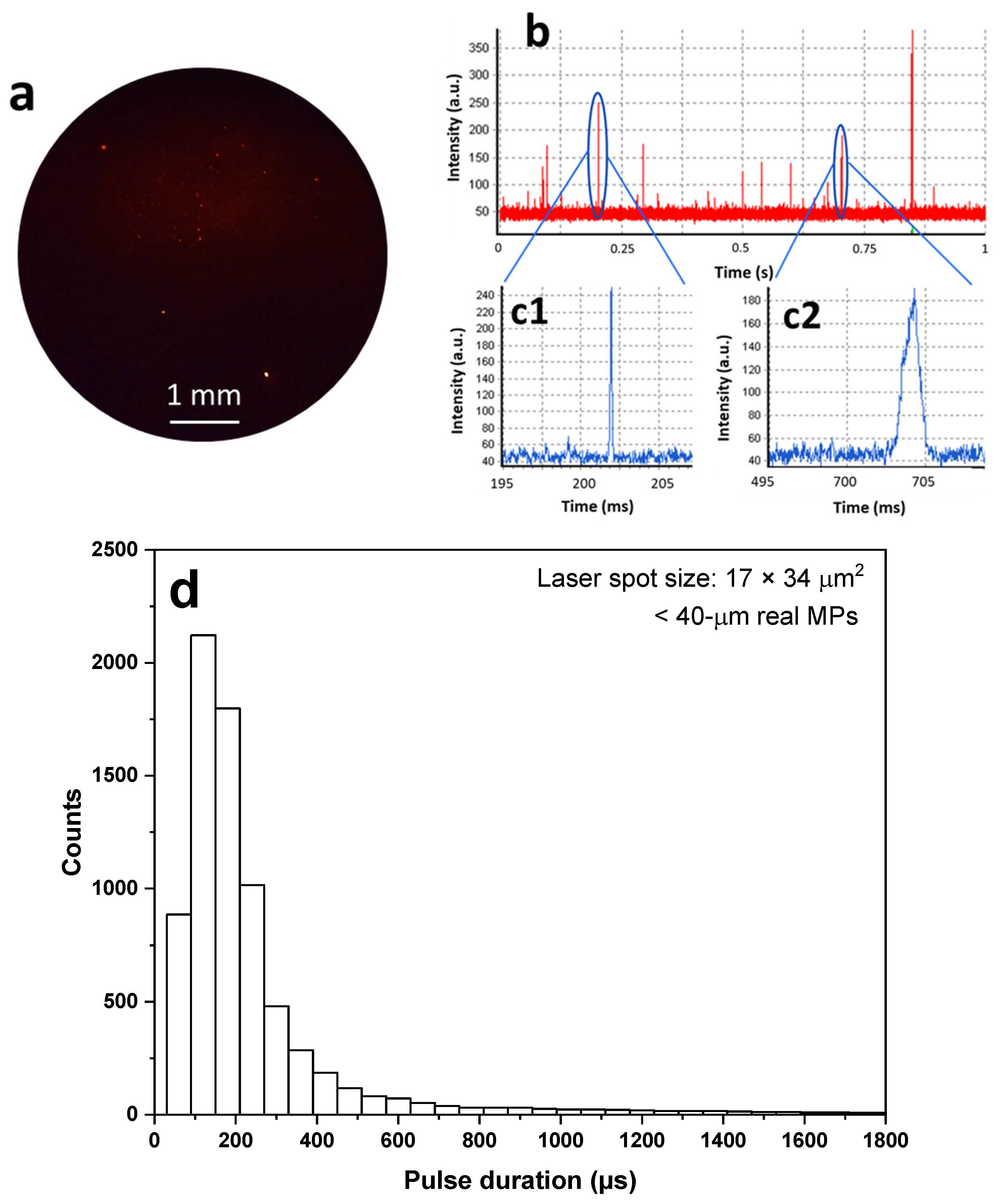
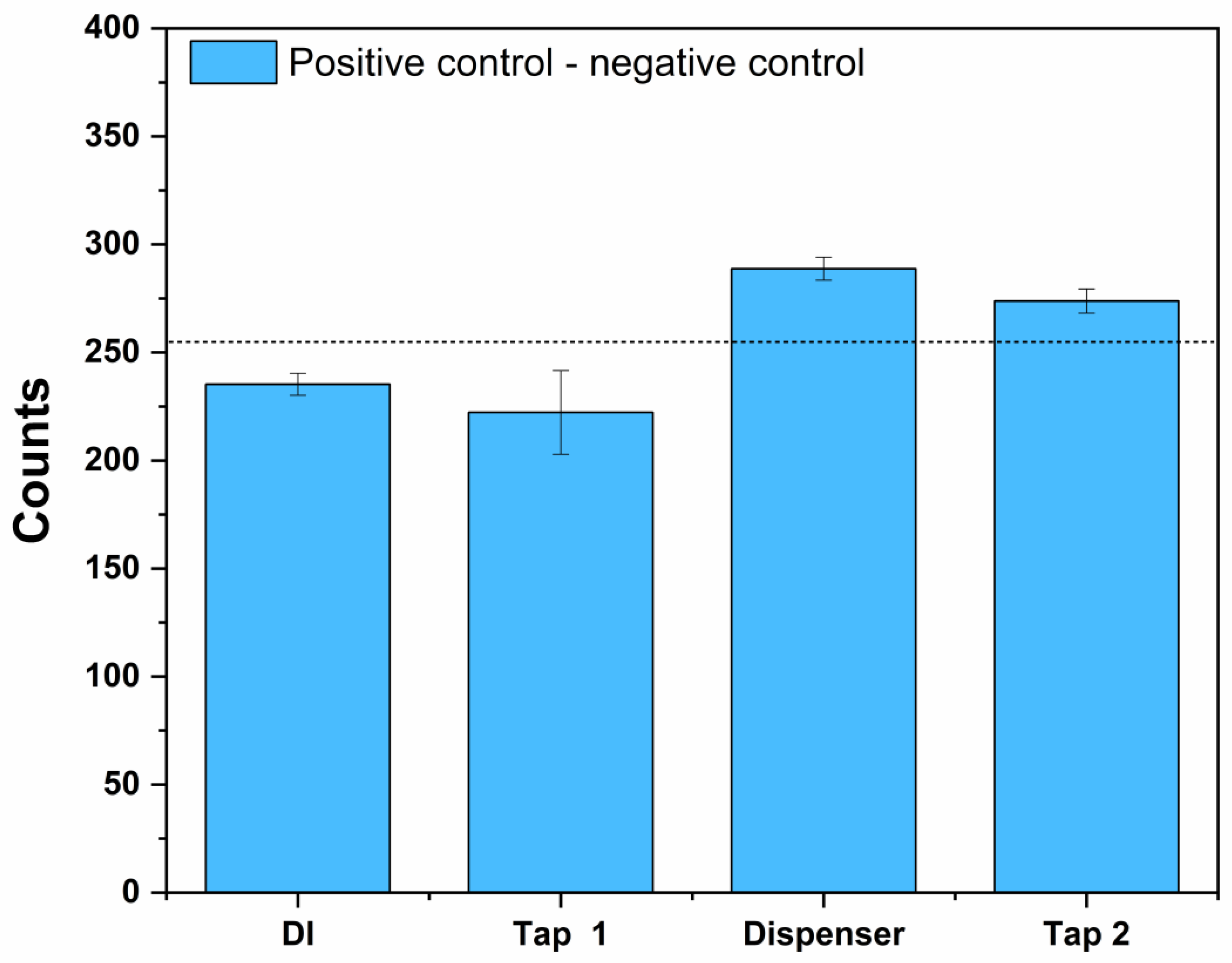
3.4. Results with Real MPs in DI and Tap Water

After the calibration with commercial fluorescent microspheres, the performance of the present method was tested under conditions more similar to the ones of real applications. For this purpose, three types of tap and drinking waters were spiked with Nile-Red-stained PS MPs with the procedure described in Section 2.2. The microscopic image in Figure 6a shows the size difference of the stained particles and Figure 6b shows the typical time-dependent electrical signal produced by the fluorescence emission in these water samples. The average pulse intensity is clearly lower than that reported in Figure 2 since the staining procedure only affects the particle surface and is less effective than the bulk dyeing performed in OFPS microspheres. Moreover, the presence of a noisy baseline likely indicates the presence of water-dispersed NR. The characteristics of pulse duration distribution (Figure 6c) are in between those of Figure 2c, thus suggesting the presence of a certain range of particle dimensions.
Figure 7 reports the difference of positive control minus negative control, as defined in Materials and Methods, which can be attributed to the spiked MPs without the false counts coming from the aggregation of NR in water [54]. The data are reported for the different real water samples in comparison with the data for DI water. Negative control counts are reported in Supplementary Materials (Figure S4). The results of Figure 7 show some variations among the different types of water, which are significantly lower than those observed in unfiltered water either with an NR concentration of 5 mg/L or 0.1 mg/L (Figure S5 and Figure S6, respectively). This is consistent with the hypothesis that an observable quantity of microplastics was originally present in real water samples.

4. Conclusions

In the present study, we propose an optical setup based on fluorescence signal recognition to realize a fast, portable, and user-friendly device for the quantitative detection of MPs in water. This preliminary work was mainly focused on proving the feasibility of the approach.
Although the agreement with theoretical predictions was slightly worse in the case of real water samples in comparison with results with calibrated commercial fluorescent microspheres, the present study demonstrated the proof of concept of a method for quick automated MP counting in water. We demonstrated that the proposed setup has the potential to discriminate MPs in real water. It should be considered that water samples from lakes, rivers, and wastewater treatment plants can have a much greater amount of organic matter, and thus a much higher fluorescence background. However, that is a common problem to visual observation and, for this reason, a large variety of pre-treatment processes based on digestion, etc., have long been developed as largely discussed and explained in the literature. Further study and setup development could also lead to the possibility of discriminating MPs in terms of size and material. In our opinion, this technology has the potential to provide a reliable and objective method for the quantitative identification of MPs in water, which could have significant implications for environmental and human health.

Supplementary Materials

The following supporting information can be downloaded at: https://www.mdpi.com/article/10.3390/photonics10050508/s1, Figure S1: Experimental counts as a function of particle number density for different values of flow rate; Figure S2: Experimental results for 10 μm OFPS microspheres at a flow rate of 10 mL/h. Theoretical distribution calculated according to Equation (S5) with no free parameters; Figure S3: Experimental results for 10 μm OFPS microspheres at a flow rate of 10 mL/h. Theoretical distribution calculated according to Equation (S5) with vM as a free adjustable parameter; Figure S4: Observed counts in spiking experiment of stained PS MPs in different types of real water and in DI water. Water was filtered through a 0.7 μm filter and NR concentration was 0.1 mg/L; Figure S5: Observed counts in spiking experiment of stained PS MPs in different types of real water and in DI water. Water was filtered through a 40 μm filter and NR concentration was 5 mg/L; Figure S6: Observed counts in spiking experiment of stained PS MPs in different types of real water and in DI water. Water was filtered through a 40 μm filter and NR concentration was 0.1 mg/L. Figure S7: The absorption (blue curve) and emission spectrum (red curve) of Nile Red used in the present study; Figure S8: The spectral response (red curve) of the H10721-110 Hamamatsu photomultiplier used in the present study; Figure S9: The transmission/reflection curves of the dichroic mirror Thorlabs DMLP550L used in the present study; Figure S10: The transmission curve of the long-pass filter Thorlabs FEL0550 used in the present study.

Author Contributions

Conceptualization, R.P. and E.N.; methodology, R.P.; formal analysis, Y.L. and R.P.; investigation, Y.L. and E.N.; writing—original draft preparation, Y.L., R.P. and E.N.; writing—review and editing, R.P. and E.N.; supervision, E.N. All authors have read and agreed to the published version of the manuscript.

Funding

This research received external funding by Resind srl (Rome, Italy). N.: 0001270, 27 May 2022.

Institutional Review Board Statement

Not applicable.

Informed Consent Statement

Not applicable.

Data Availability Statement

Not applicable.

Conflicts of Interest

The authors declare no conflict of interest.

References

  1. Ryan, P.G.; Moloney, C.L. Plastic and Other Artefacts on South African Beaches: Temporal Trends in Abundance and Composition. S. Afr. J. Sci. 1990, 86, 450–452. [Google Scholar]
  2. Thompson, R.C.; Olsen, Y.; Mitchell, R.P.; Davis, A.; Rowland, S.J.; John, A.W.G.; McGonigle, D.; Russell, A.E. Lost at Sea: Where Is All the Plastic? Science 2004, 304, 838. [Google Scholar] [CrossRef] [PubMed]
  3. Frias, J.P.G.L.; Nash, R. Microplastics: Finding a Consensus on the Definition. Mar. Pollut. Bull. 2019, 138, 145–147. [Google Scholar] [CrossRef]
  4. Bashir, S.M.; Kimiko, S.; Mak, C.W.; Fang, J.K.H.; Gonçalves, D. Personal Care and Cosmetic Products as a Potential Source of Environmental Contamination by Microplastics in a Densely Populated Asian City. Front. Mar. Sci. 2021, 8, 683482. [Google Scholar] [CrossRef]
  5. Castelvetro, V.; Corti, A.; Biale, G.; Ceccarini, A.; Degano, I.; La Nasa, J.; Lomonaco, T.; Manariti, A.; Manco, E.; Modugno, F.; et al. New Methodologies for the Detection, Identification, and Quantification of Microplastics and Their Environmental Degradation by-Products. Environ. Sci. Pollut. Res. 2021, 28, 46764–46780. [Google Scholar] [CrossRef]
  6. He, D.; Bristow, K.; Filipović, V.; Lv, J.; He, H. Microplastics in Terrestrial Ecosystems: A Scientometric Analysis. Sustainability 2020, 12, 8739. [Google Scholar] [CrossRef]
  7. Campanale, C.; Galafassi, S.; Savino, I.; Massarelli, C.; Ancona, V.; Volta, P.; Uricchio, V.F. Microplastics Pollution in the Terrestrial Environments: Poorly Known Diffuse Sources and Implications for Plants. Sci. Total Environ. 2022, 805, 150431. [Google Scholar] [CrossRef]
  8. Dissanayake, P.D.; Kim, S.; Sarkar, B.; Oleszczuk, P.; Sang, M.K.; Haque, M.N.; Ahn, J.H.; Bank, M.S.; Ok, Y.S. Effects of Microplastics on the Terrestrial Environment: A Critical Review. Environ. Res. 2022, 209, 112734. [Google Scholar] [CrossRef]
  9. Zhang, T.; Jiang, B.; Xing, Y.; Ya, H.; Lv, M.; Wang, X. Current Status of Microplastics Pollution in the Aquatic Environment, Interaction with Other Pollutants, and Effects on Aquatic Organisms. Environ. Sci. Pollut. Res. 2022, 1, 3. [Google Scholar] [CrossRef]
  10. Xiang, Y.; Jiang, L.; Zhou, Y.; Luo, Z.; Zhi, D.; Yang, J.; Lam, S.S. Microplastics and Environmental Pollutants: Key Interaction and Toxicology in Aquatic and Soil Environments. J. Hazard. Mater. 2022, 422, 126843. [Google Scholar] [CrossRef] [PubMed]
  11. Li, J.; Liu, H.; Paul Chen, J. Microplastics in Freshwater Systems: A Review on Occurrence, Environmental Effects, and Methods for Microplastics Detection. Water Res. 2018, 137, 362–374. [Google Scholar] [CrossRef]
  12. Chen, G.; Fu, Z.; Yang, H.; Wang, J. An Overview of Analytical Methods for Detecting Microplastics in the Atmosphere. TrAC Trends Anal. Chem. 2020, 130, 115981. [Google Scholar] [CrossRef]
  13. Munyaneza, J.; Jia, Q.; Qaraah, F.A.; Hossain, M.F.; Wu, C.; Zhen, H.; Xiu, G. A Review of Atmospheric Microplastics Pollution: In-Depth Sighting of Sources, Analytical Methods, Physiognomies, Transport and Risks. Sci. Total Environ. 2022, 822, 153339. [Google Scholar] [CrossRef]
  14. Habibi, N.; Uddin, S.; Fowler, S.W.; Behbehani, M. Microplastics in the Atmosphere: A Review. J. Environ. Expo. Assess. 2022, 1, 6. [Google Scholar] [CrossRef]
  15. Rota, E.; Bergami, E.; Corsi, I.; Bargagli, R. Macro- and Microplastics in the Antarctic Environment: Ongoing Assessment and Perspectives. Environments 2022, 9, 93. [Google Scholar] [CrossRef]
  16. Lusher, A.L.; Tirelli, V.; O’Connor, I.; Officer, R. Microplastics in Arctic Polar Waters: The First Reported Values of Particles in Surface and Sub-Surface Samples. Sci. Rep. 2015, 5, 14947. [Google Scholar] [CrossRef]
  17. Rodrigues, S.M.; Elliott, M.; Almeida, C.M.R.; Ramos, S. Microplastics and Plankton: Knowledge from Laboratory and Field Studies to Distinguish Contamination from Pollution. J. Hazard. Mater. 2021, 417, 126057. [Google Scholar] [CrossRef]
  18. Li, J.; Lusher, A.L.; Rotchell, J.M.; Deudero, S.; Turra, A.; Bråte, I.L.N.; Sun, C.; Shahadat Hossain, M.; Li, Q.; Kolandhasamy, P.; et al. Using Mussel as a Global Bioindicator of Coastal Microplastic Pollution. Environ. Pollut. 2019, 244, 522–533. [Google Scholar] [CrossRef] [PubMed]
  19. Korez, Š.; Gutow, L.; Saborowski, R. Coping with the “Dirt”: Brown Shrimp and the Microplastic Threat. Zoology 2020, 143, 125848. [Google Scholar] [CrossRef] [PubMed]
  20. Yoon, H.; Park, B.; Rim, J.; Park, H. Detection of Microplastics by Various Types of Whiteleg Shrimp (Litopenaeus vannamei) in the Korean Sea. Separations 2022, 9, 332. [Google Scholar] [CrossRef]
  21. Hernandez-Gonzalez, A.; Saavedra, C.; Gago, J.; Covelo, P.; Santos, M.B.; Pierce, G.J. Microplastics in the Stomach Contents of Common Dolphin (Delphinus delphis) Stranded on the Galician Coasts (NW Spain, 2005–2010). Mar. Pollut. Bull. 2018, 137, 526–532. [Google Scholar] [CrossRef] [PubMed]
  22. Parton, K.J.; Godley, B.J.; Santillo, D.; Tausif, M.; Omeyer, L.C.M.; Galloway, T.S. Investigating the Presence of Microplastics in Demersal Sharks of the North-East Atlantic. Sci. Rep. 2020, 10, 12204. [Google Scholar] [CrossRef] [PubMed]
  23. Moore, R.C.; Loseto, L.; Noel, M.; Etemadifar, A.; Brewster, J.D.; MacPhee, S.; Bendell, L.; Ross, P.S. Microplastics in Beluga Whales (Delphinapterus leucas) from the Eastern Beaufort Sea. Mar. Pollut. Bull. 2020, 150, 110723. [Google Scholar] [CrossRef]
  24. Kim, J.S.; Lee, H.J.; Kim, S.K.; Kim, H.J. Global Pattern of Microplastics (MPs) in Commercial Food-Grade Salts: Sea Salt as an Indicator of Seawater MP Pollution. Environ. Sci. Technol. 2018, 52, 12819–12828. [Google Scholar] [CrossRef] [PubMed]
  25. Afrin, S.; Rahman, M.M.; Hossain, M.N.; Uddin, M.K.; Malafaia, G. Are There Plastic Particles in My Sugar? A Pioneering Study on the Characterization of Microplastics in Commercial Sugars and Risk Assessment. Sci. Total Environ. 2022, 837, 155849. [Google Scholar] [CrossRef] [PubMed]
  26. Kutralam-Muniasamy, G.; Pérez-Guevara, F.; Elizalde-Martínez, I.; Shruti, V.C. Branded Milks—Are They Immune from Microplastics Contamination? Sci. Total Environ. 2020, 714, 136823. [Google Scholar] [CrossRef]
  27. Mason, S.A.; Welch, V.G.; Neratko, J. Synthetic Polymer Contamination in Bottled Water. Front. Chem. 2018, 6, 407. [Google Scholar] [CrossRef]
  28. Kosuth, M.; Mason, S.A.; Wattenberg, E.V. Anthropogenic Contamination of Tap Water, Beer, and Sea Salt. PLoS ONE 2018, 13, e0194970. [Google Scholar] [CrossRef]
  29. Kedzierski, M.; Lechat, B.; Sire, O.; Le Maguer, G.; Le Tilly, V.; Bruzaud, S. Microplastic Contamination of Packaged Meat: Occurrence and Associated Risks. Food Packag. Shelf Life 2020, 24, 100489. [Google Scholar] [CrossRef]
  30. Jinhui, S.; Sudong, X.; Yan, N.; Xia, P.; Jiahao, Q.; Yongjian, X. Effects of Microplastics and Attached Heavy Metals on Growth, Immunity, and Heavy Metal Accumulation in the Yellow Seahorse, Hippocampus Kuda Bleeker. Mar. Pollut. Bull. 2019, 149, 110510. [Google Scholar] [CrossRef]
  31. He, L.; Wu, D.; Rong, H.; Li, M.; Tong, M.; Kim, H. Influence of Nano- and Microplastic Particles on the Transport and Deposition Behaviors of Bacteria in Quartz Sand. Environ. Sci. Technol. 2018, 52, 11555–11563. [Google Scholar] [CrossRef]
  32. Moresco, V.; Oliver, D.M.; Weidmann, M.; Matallana-Surget, S.; Quilliam, R.S. Survival of Human Enteric and Respiratory Viruses on Plastics in Soil, Freshwater, and Marine Environments. Environ. Res. 2021, 199, 111367. [Google Scholar] [CrossRef] [PubMed]
  33. Prata, J.C.; da Costa, J.P.; Lopes, I.; Duarte, A.C.; Rocha-Santos, T. Environmental Exposure to Microplastics: An Overview on Possible Human Health Effects. Sci. Total Environ. 2020, 702, 134455. [Google Scholar] [CrossRef] [PubMed]
  34. Huang, W.; Song, B.; Liang, J.; Niu, Q.; Zeng, G.; Shen, M.; Deng, J.; Luo, Y.; Wen, X.; Zhang, Y. Microplastics and Associated Contaminants in the Aquatic Environment: A Review on Their Ecotoxicological Effects, Trophic Transfer, and Potential Impacts to Human Health. J. Hazard. Mater. 2021, 405, 124187. [Google Scholar] [CrossRef] [PubMed]
  35. Jiang, B.; Kauffman, A.E.; Li, L.; McFee, W.; Cai, B.; Weinstein, J.; Lead, J.R.; Chatterjee, S.; Scott, G.I.; Xiao, S. Health Impacts of Environmental Contamination of Micro- and Nanoplastics: A Review. Environ. Health Prev. Med. 2020, 25, 29. [Google Scholar] [CrossRef]
  36. Asamoah, B.O.; Kanyathare, B.; Roussey, M.; Peiponen, K.E. A Prototype of a Portable Optical Sensor for the Detection of Transparent and Translucent Microplastics in Freshwater. Chemosphere 2019, 231, 161–167. [Google Scholar] [CrossRef]
  37. Iri, A.H.; Shahrah, M.H.A.; Ali, A.M.; Qadri, S.A.; Erdem, T.; Ozdur, I.T.; Icoz, K. Optical Detection of Microplastics in Water. Environ. Sci. Pollut. Res. 2021, 28, 63860–63866. [Google Scholar] [CrossRef]
  38. Nicolai, E.; Pizzoferrato, R.; Li, Y.; Frattegiani, S.; Nucara, A.; Costa, G. A New Optical Method for Quantitative Detection of Microplastics in Water Based on Real-Time Fluorescence Analysis. Water 2022, 14, 3235. [Google Scholar] [CrossRef]
  39. Mesquita, P.; Gong, L.; Lin, Y. A Low-Cost Microfluidic Method for Microplastics Identification: Towards Continuous Recognition. Micromachines 2022, 13, 499. [Google Scholar] [CrossRef]
  40. Lin, Y.H.; Chang, C.H. Glass Capillary Assembled Microfluidic Three-Dimensional Hydrodynamic Focusing Device for Fluorescent Particle Detection. Microfluid. Nanofluid. 2021, 25, 42. [Google Scholar] [CrossRef]
  41. Sturm, M.T.; Horn, H.; Schuhen, K. The Potential of Fluorescent Dyes—Comparative Study of Nile Red and Three Derivatives for the Detection of Microplastics. Anal. Bioanal. Chem. 2021, 413, 1059–1071. [Google Scholar] [CrossRef] [PubMed]
  42. Liu, S.; Shang, E.; Liu, J.; Wang, Y.; Bolan, N.; Kirkham, M.B.; Li, Y. What Have We Known so Far for Fluorescence Staining and Quantification of Microplastics: A Tutorial Review. Front. Environ. Sci. Eng. 2022, 16, 8. [Google Scholar] [CrossRef]
  43. Meyers, N.; Catarino, A.I.; Declercq, A.M.; Brenan, A.; Devriese, L.; Vandegehuchte, M.; De Witte, B.; Janssen, C.; Everaert, G. Microplastic Detection and Identification by Nile Red Staining: Towards a Semi-Automated, Cost- and Time-Effective Technique. Sci. Total Environ. 2022, 823, 153441. [Google Scholar] [CrossRef] [PubMed]
  44. Karakolis, E.G.; Nguyen, B.; You, J.B.; Rochman, C.M.; Sinton, D. Fluorescent Dyes for Visualizing Microplastic Particles and Fibers in Laboratory-Based Studies. Environ. Sci. Technol. Lett. 2019, 6, 334–340. [Google Scholar] [CrossRef]
  45. Shim, W.J.; Song, Y.K.; Hong, S.H.; Jang, M. Identification and Quantification of Microplastics Using Nile Red Staining. Mar. Pollut. Bull. 2016, 113, 469–476. [Google Scholar] [CrossRef]
  46. Konde, S.; Ornik, J.; Prume, J.A.; Taiber, J.; Koch, M. Exploring the Potential of Photoluminescence Spectroscopy in Combination with Nile Red Staining for Microplastic Detection. Mar. Pollut. Bull. 2020, 159, 111475. [Google Scholar] [CrossRef]
  47. Nicolai, E.; Garau, S.; Favalli, C.; D’Agostini, C.; Gratton, E.; Motolese, G.; Rosato, N. Evaluation of BiesseBioscreen as a New Methodology for Bacteriuria Screening. New Microbiol. 2014, 37, 495–501. [Google Scholar]
  48. Nicolai, E.; Pieri, M.; Gratton, E.; Motolese, G.; Bernardini, S. Bacterial Infection Diagnosis and Antibiotic Prescription in 3 h as an Answer to Antibiotic Resistance: The Case of Urinary Tract Infections. Antibiotics 2021, 10, 1168. [Google Scholar] [CrossRef]
  49. Toosky, M.N.; Grunwald, J.T.; Pala, D.; Shen, B.; Zhao, W.; D’agostini, C.; Coghe, F.; Angioni, G.; Motolese, G.; Abram, T.J.; et al. A Rapid, Point-of-Care Antibiotic Susceptibility Test for Urinary Tract Infections. J. Med. Microbiol. 2020, 69, 52–62. [Google Scholar] [CrossRef]
  50. Suzaki, Y.; Tachibana, A. Measurement of the Μm Sized Radius of Gaussian Laser Beam Using the Scanning Knife-Edge. Appl. Opt. 1975, 14, 2809. [Google Scholar] [CrossRef]
  51. Al-Azzawi, M.S.M.; Kunaschk, M.; Mraz, K.; Freier, K.P.; Knoop, O.; Drewes, J.E. Digest, Stain and Bleach: Three Steps to Achieving Rapid Microplastic Fluorescence Analysis in Wastewater Samples. Sci. Total Environ. 2023, 863, 160947. [Google Scholar] [CrossRef] [PubMed]
  52. Zhou, F.; Wang, X.; Wang, G.; Zuo, Y. A Rapid Method for Detecting Microplastics Based on Fluorescence Lifetime Imaging Technology (FLIM). Toxics 2022, 10, 118. [Google Scholar] [CrossRef] [PubMed]
  53. Shruti, V.C.; Pérez-Guevara, F.; Roy, P.D.; Kutralam-Muniasamy, G. Analyzing Microplastics with Nile Red: Emerging Trends, Challenges, and Prospects. J. Hazard. Mater. 2022, 423, 127171. [Google Scholar] [CrossRef] [PubMed]
  54. Hernandez, L.M.; Farner, J.M.; Claveau-Mallet, D.; Okshevsky, M.; Jahandideh, H.; Matthews, S.; Roy, R.; Yaylayan, V.; Tufenkji, N. Optimizing the Concentration of Nile Red for Screening of Microplastics in Drinking Water. ACS ES&T Water 2023, 3, 1029–1038. [Google Scholar] [CrossRef]
  55. Kunst, B.H.; Schots, A.; Visser, A.J.W.G. Detection of Flowing Fluorescent Particles in a Microcapillary Using Fluorescence Correlation Spectroscopy. Anal. Chem. 2002, 74, 5350–5357. [Google Scholar] [CrossRef]
Figure 1. Schematic of the optical setup.
Photonics 10 00508 g001
Figure 2. (a) Microscopic observation of 10 µm OFPS microspheres; (b) the electrical signal corresponding to the typical fluorescence time profile for the OFPS microspheres sample; (c1,c2) two representative pulses are reported on a larger time scale along with the matching to a Gaussian pattern (red lines). (d) Time duration distribution of the pulses recorded during a 60 s measurement. The red continuous line is the prediction of the model described in Supplementary Information.
Photonics 10 00508 g002
Figure 3. Experimental counts as a function of particle number density compared with the predicted values according to laminar flow and measured concentration.
Photonics 10 00508 g003
Figure 4. (a) Experimental counts as a function of flow rate. (b) Pulse duration distribution as a function of flow rate.
Photonics 10 00508 g004
Figure 5. Distribution of pulse time duration recorded with different dimensions of the laser spot (a) for 10 µm and (b) for 1 µm PS microspheres.
Photonics 10 00508 g005
Figure 6. (a) Microscopic observation of real < 40 μm NR-stained PS MPs; (b) the electrical signal corresponding to the typical fluorescence time profile; (c1,c2) two representative pulses are reported on a larger time scale; (d) the pulse duration distribution of the pulses recorded during a 60 s measurement.
Photonics 10 00508 g006
Figure 7. Observed counts in spiking experiment of stained PS MPs in different types of real water and in DI water, pre-filtered with a 0.7 μm pore size filter. N = 5 and the error bars are ±σ. The horizontal dashed bar represents the average values of counts over the different samples.
Photonics 10 00508 g007
Disclaimer/Publisher’s Note: The statements, opinions and data contained in all publications are solely those of the individual author(s) and contributor(s) and not of MDPI and/or the editor(s). MDPI and/or the editor(s) disclaim responsibility for any injury to people or property resulting from any ideas, methods, instructions or products referred to in the content.

