Article

A Lightweight Swin Transformer-Based Pipeline for Optical Coherence Tomography Image Denoising in Skin Application

Centre of Medical Engineering and Technology, School of Science and Engineering, University of Dundee, Dundee DD1 4HN, UK
*
Author to whom correspondence should be addressed.
Photonics 2023, 10(4), 468; https://doi.org/10.3390/photonics10040468
Submission received: 17 March 2023 / Revised: 13 April 2023 / Accepted: 18 April 2023 / Published: 19 April 2023
(This article belongs to the Special Issue High-Performance Optical Coherence Tomography)

Abstract

:
Optical coherence tomography (OCT) has attracted attention in dermatology applications for skin disease characterization and diagnosis because it provides high-resolution (<10 μm) of tissue non-invasively with high imaging speed (2–8 s). However, the quality of OCT images can be significantly degraded by speckle noise, which results from light waves scattering in multiple directions. This noise can hinder the accuracy of disease diagnosis, and the conventional frame averaging method requires multiple repeated (e.g., four to six) scans, which is time consuming and introduces motion artifacts. To overcome these limitations, we proposed a lightweight U-shape Swin (LUSwin) transformer-based denoising pipeline to recover high-quality OCT images from the noisy OCT images by utilizing a fast one-repeated OCT scan. In terms of the peak signal-to-noise-ratio (PSNR) performance, the results reveal that the denoised images from the LUSwin transformer (26.92) are of a higher quality than the four-repeated frame-averaging method (26.19). Compared to the state-of-the-art networks in image denoising, the proposed LUSwin transformer has the smallest floating points operation (3.9299 G) and has the second highest PSNR results, only 0.02 lower than the Swin-UNet, which has the highest PSNR results (26.94). This study demonstrates that the transformer model has the capacity to denoise the noisy OCT image from a fast one-repeated OCT scan.

1. Introduction

The skin is the largest organ in direct contact with the external environment and is the first barrier to preventing the entry of harmful substances into the bodies of humans and other vertebrates [1]. In dermatology clinics, the diagnosis of a skin disease usually relies on physical examination, followed by a histological biopsy. Nevertheless, a skin biopsy is an invasive method that can be performed by shaving, punching, or incision to obtain sufficient tissue volume for interpretation, which is low repeatable and brings injury to the patients. Optical coherence tomography (OCT) is a non-invasive, label-free, real-time in vivo imaging device. With broadband LASERs in infrared wavelength, the OCT can provide micron-level resolution (~5 μm) tomographic images with depth information up to 3 mm in biology tissue [2]. Through analyses of skin signatures (definition of the epidermal–dermal junction, ovoid structures, etc.), most studies confirmed OCT significantly improved the sensitivity and specificity [3,4,5,6]. However, the speckle noise in the OCT scan seriously degraded the quality and contrast of the skin structures in the OCT image, reducing the accuracy of the skin disease diagnoses [7]. It is a challenge to recover the high-quality OCT structure image from the speckle noise. High-repeated (e.g., four to six repeated) OCT scans in the same location are a common method to suppress the noise in the OCT image [8]. However, this method introduces motion artifacts to images because of the longer scan time, while reducing the repeated scan (e.g., one-repeated) can lead to low contrast and high speckle noise results. Regarding the denoising algorithms, a series of denoising filters were applied to the OCT images to reduce the speckle noise [9,10]. However, these filters are complexly designed and might remove the slight skin tissue signal, losing the high-frequency details (low sharpness) of the images [11].
Recently, based on convolution neural networks (CNN), a series of neural networks with different architectures were proposed to denoise the high-quality OCT images from the counterpart low-quality image [11,12,13,14,15]. These methods achieved good competitive results in OCT image denoising but cannot meet the requirement of high-quality OCT image denoising and reconstruction. Since the CNN-type model is based on the convolution operation, which has a limited receptive field (e.g., 3 × 3) and is based on the local feature extraction, it cannot learn long-term information during the image denoising. Moreover, due to the convolution operation, the checkboard-like artifacts will be obvious in the denoised and reconstructed images if using the deconvolution layer, such as the encoder–decoder architecture model [16]. In terms of the application, current research is focused on the retina OCT images denoising in the field of ophthalmology; hence, rather than solely concentrating on reducing noise, the CNN model must relearn the different signatures from skin OCT structure images in dermatology.
By flattening the 2-dimensional (2D) image into 1-dimension (1D) sequences, a vision transformer (ViT) can provide good performance in image classification by using a large receipt field (i.e., 16 × 16) and global information [17]. However, a large amount of data (e.g., 300 M images JFT300 datasets) are required for ViT fine-tuning and training. By introducing the hierarchical shifted windows (Swin) into the transformer, the Swin transformer can better utilize the neighbor content information and achieve a better performance than the ViT in the ImageNet2K classification task [18]. With the Swin transformer, Swin-IR was proposed for image restoration and achieved a better performance than the CNN-based methods in natural image reconstruction and super resolution. By combining the encoder–decoder architecture and the Swin transformer, Swin-UNet [19] achieved a good performance in medical image segmentation, while the requirement of the computation cost is lower than that of the Swin-IR. Compared with the U-Net [20], the fully connected layer took the place of the deconvolution layer to upscale the shape of the feature maps, reducing the potential checkboard-like artifacts. However, the network size of Swin-IR and Swin-UNet is so large that it requires a high computational resource. Additionally, Swin-UNet was first proposed for segmentation, which is different from denoising. Hence, a lightweight model is desired to reduce the computational cost while providing high denoising performance.
Inspired by the success of the Swin transformer and Swin U-Net, this paper proposes a lightweight U-shape Swin (LUSwin) transformer model that allows the developer to use a low-computational cost network for OCT image denoising, and the denoising and network training pipeline is shown in Figure 1. The LUSwin Transformer has an encoder–decoder architecture that allows for efficient learning. To improve the network generalization of the noise reduction, the OCT images from a series of positions of the skin with various textures and signatures were collected from the participants. Concretely, our contributions can be summarized as follows: (1) We proposed a low computational cost pipeline to enhance the image quality of the noisy OCT skin image based on the fast one-repeated OCT scan. (2) Based on the Swin transformer, we proposed an LUSwin transformer, which has a symmetric encoder–decoder architecture and less computational cost than U-Net and Swin-UNet, to denoise the skin OCT images. (3) We conducted an investigation of the perceptual loss on the neural network training for skin OCT image denoising. (4). A comparative study between the CNN- and transformer-type models in skin OCT image denoising was performed.

2. Materials and Methods

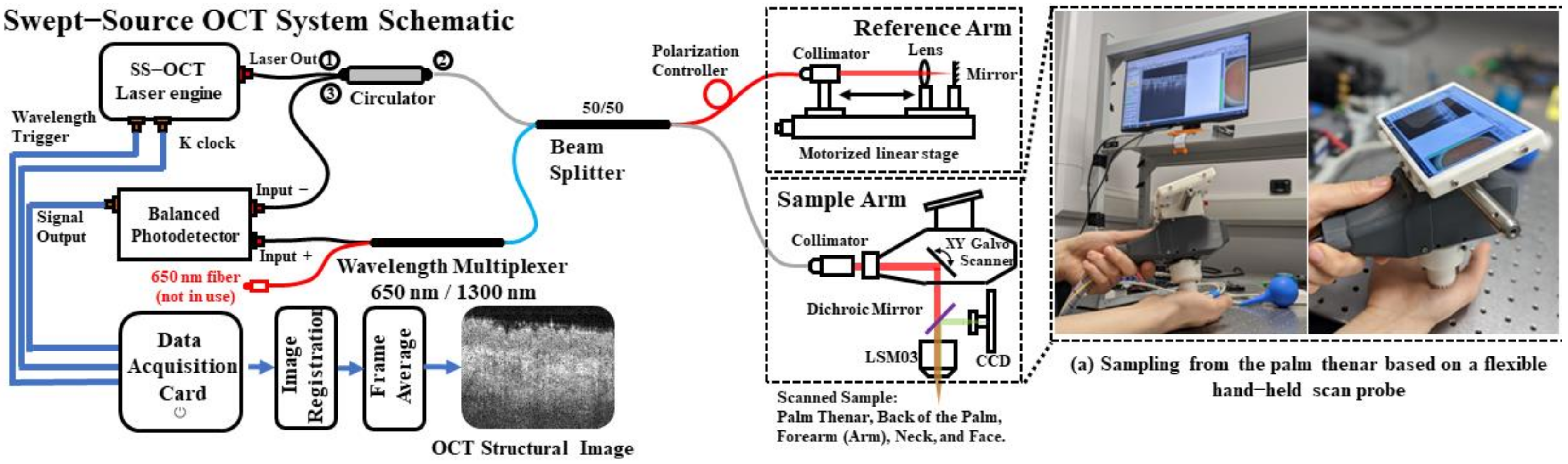
2.1. Swept-Source OCT and Data Acquisition

A lab-built swept-source OCT (SSOCT) system was utilized to non-invasively visualize the skin structure with a hand-held probe, and Figure 2 shows the system schematic of the SSOCT used in this study. The swept-source laser (SL132120, Thorlabs Inc., Newton, MA, USA) used in this system has a wavelength of 1310 nm, a bandwidth of 100 nm, and a 200 kHz swept rate. More details of the SSOCT system are described in [21]. This system has a theoretical axial resolution of 7.4 μm in air, and the penetration depth of skin with this system is ~2 mm.
Regarding the data acquisition from the participants, a hand-held scan probe was used during the data sampling to simulate the clinic data acquisition procedure, as described in Figure 2a. The scan positions were palm thenar, back of the palm, forearm (arms), neck, and face for each participant. The selected positions are areas that are easily exposed to sunshine, which means skin diseases are prominent in these areas [22]. To reduce the influence of the motion artifacts between the hand-held probe and the participants, each position was scanned three times, and high-quality data with the least motion artifacts were manually selected. To further eliminate motion artifacts in human skin, an image registration method, including rigid affine and non-rigid B-spline, was applied based on the Matlab (MathWorks, Inc., Natick, MA, USA) open-source image registration toolbox Elastix [23,24]. Regarding the scanning protocol to obtain six-repeated OCT signals, each OCT volume has a size of 6 × 600 × 600 × 300 (n, x, y, z), where n is the repeated scans of the OCT volume, x and y are the transverse axis, and z is the axial axis. The field of view was set at approximately 5 mm × 5 mm. There were sixteen healthy participants ranging in age from 20 to 35, none of whom had any skin disease or skin condition. After the data acquisition and manual selection to remove low-quality OCT data, a total of 29 six-repeated OCT signals were collected from the participants, and the details of the OCT signals are shown in Table 1.
In terms of image pre-processing for network training, the image registration and frame average algorithms mentioned above were used to generate high-quality OCT images based on the six-repeated OCT signals. In the meantime, the noisy image was generated based on the first volume (size is 1 × 600 × 600 × 300 (n, x, y, z)) of each six-repeated OCT signal. With a split rate of 0.8 for the training data and 0.2 for the validation data, 6 independent OCT signals from #004, #005, #011, and #014 were used to generate the validation data, and the remaining 23 OCT signals were used to generate the training data. Then, the processed high-quality and noisy OCT images were split into 2D B-frame (600 × 300) images. Considering that the shape of one B-frame image is too large for neural network training with a GTX1080 Ti graphics card (11 GB) in this study, each B-frame image was split into three 192 × 192 images to prevent the out-of-memory situation. Finally, a total of 52,200 B-frame images were extracted as high-quality images and noisy images, respectively. Among them, 41,400 pairs of high-quality and noisy images were used as the training dataset, and the remaining 10,800 as the validation dataset.
The data acquisition of the volunteers was approved by the School of Science and Engineering Research Ethics Committee of the University of Dundee (Approval Number: UOD_SSREC_PGR_2022_003), which also conforms to the tenets of the Declaration of Helsinki. Informed consent was obtained from the participants before the data collection, and all the participants were informed that the collected data would be used in this article. The collected data were anonymized, and the participants’ identification was removed.

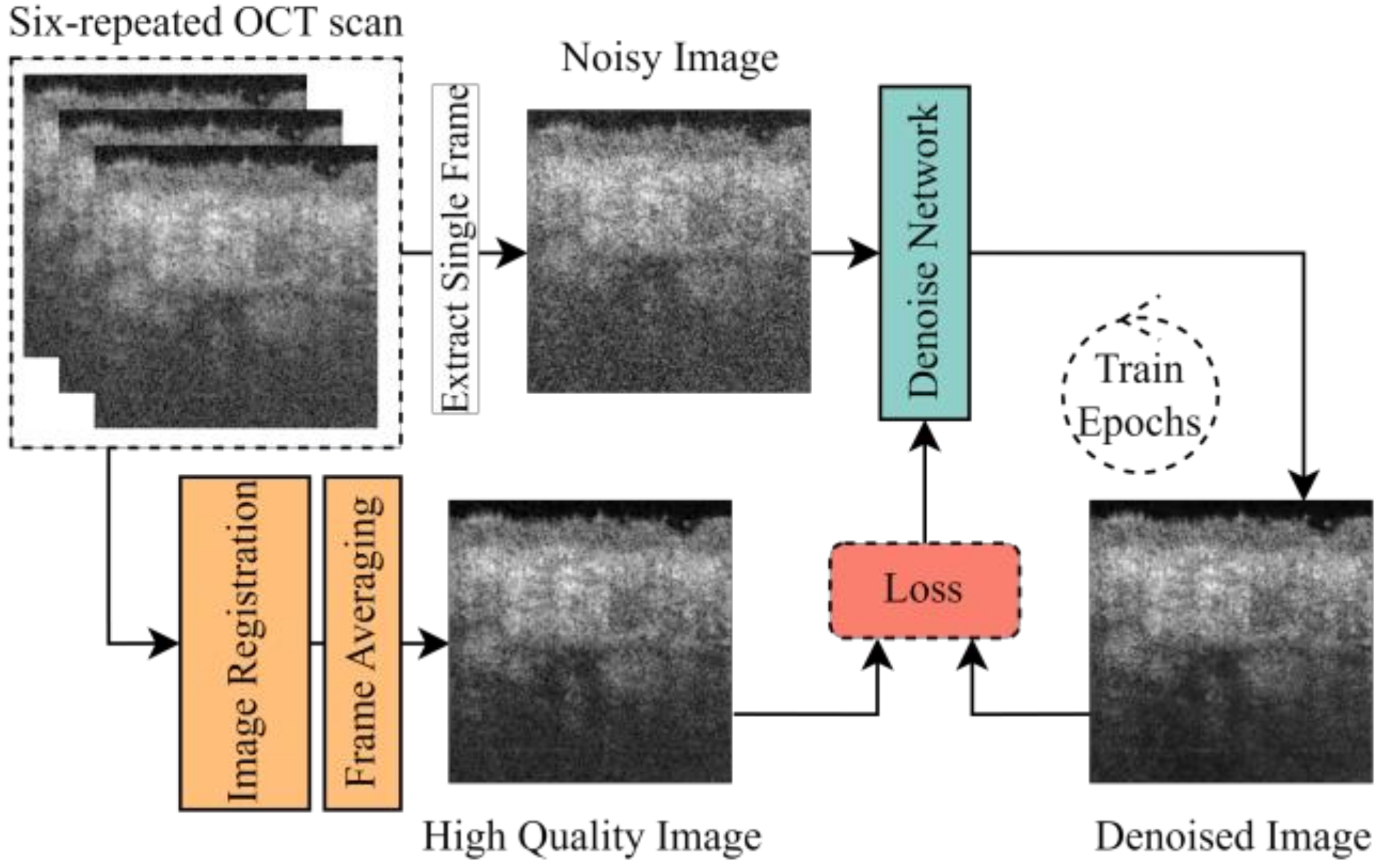
2.2. Definition of OCT Image Denoising

The data collection and pre-processing to obtain the counterpart high-quality images ( I H Q ) and noisy OCT images ( I N o i s y ) were mentioned in the above paragraph. Two types of OCT image denoising were involved in this study, those being the frame averaging and deep-learning-based methods. Assuming there is a four-repeated scan OCT signal that composes of four volumes V 1 ,   V 2 ,   V 3 , V 4 , the frame averaging method can be written as:
I f r a m e a v e r a g i n g = 1 N R i = 1 n V 1 i + V 2 i + V 3 i + V 4 i
where n represents the total pixels of the volume and V 1 i means the no. i pixel of the first volume. NR is the number of repeated scans in the OCT signal. The more repeated scans, the higher the quality of the output OCT images, but this also results in a longer data acquisition time and more unpredictable motion artifacts.
Additionally, the deep-learning-based method aims to learn the mapping relationship between the I H Q and I N o i s y and reduce the noise in the I N o i s y while maintaining significant structural signals. The denoised processing of the neural networks can be written as:
I D e n o i s e d = H W I N o i s y
where H W is the denoised neural network with trainable weights W and I D e n o i s e d is the output denoised image from the denoised network. As demonstrated in Figure 1, the I N o i s y is extracted from the single OCT scan. By calculating the loss with I H Q , the loss is then used to calculate the gradience for the neural network’s weights updating with the help of the optimizer algorithm, such as step gradient descent and Adam [25].

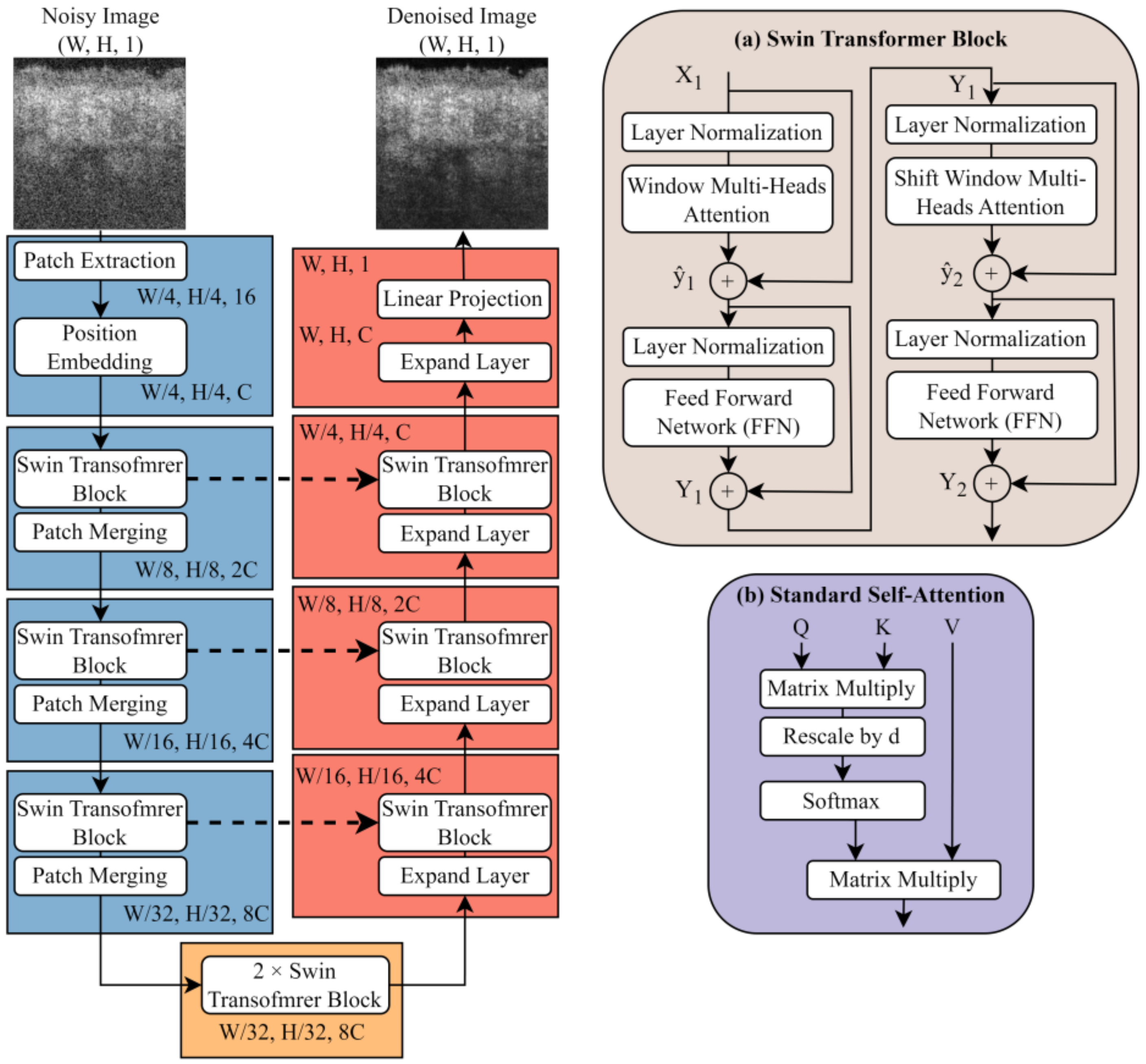
2.3. Lightweight U-Shape Swin Transformer

Figure 3 outlines the architecture of the proposed lightweight U-shape Swin (LUSwin) transformer. Assuming the shape of the LUSwin transformer model input is H × W, the first patch extraction layer will split the input image with patch size 4 × 4 without overlapping. Hence, the shape of the patch extraction layer output is H/4 × W/4 × (4 × 4). A position embedding layer with C features is then applied to the output image patches, and the output shape is H/4 × W/4 × C, where C is set as 64 in this study. The embedding output is then sent into a Swin transformer block (STB), which will not change the shape of the feature maps. In the encoder part, the patch merging layer is used to downsample the shape of the feature map and increase the feature dims of the feature map (e.g., input shape is H/4 × W/4 × C, and output shape is H/8 × W/8 × 2 C). The bottleneck has two STBs, and the output from the bottleneck is fed into the decoder. The expanded layer is aimed at upsampling the feature map and reducing the feature dims (e.g., from H/8 × W/8 × 2 C to H/4 × W/4 × C). The latest expanded layer in the decoder can 4× upsample the feature map, and the final linear projection layer has a hidden size of 1 to match the channel output.

2.3.1. Swin Transformer Block

In Figure 3a, the Swin transformer block (STB) [18,19] contains a window multi-head attention layer (WMA), a shift-windows multi-head attention layer (SWMA), a series of layer normalization (LN) layers, and two feed-forward networks (FFN). Taking X 1 as the input of the STB, the processing procedure of the STB can be written as follows:
y ^ 1 = W M A L N 1 X 1 + X 1
Y 1 = F F N 1 L N 2 y ^ 1 + y ^ 1
y ^ 2 = S W M A L N 3 Y 1 + Y 1
Y 2 = F F N 2 L N 4 y ^ 2 + y ^ 2
where FFN contains two linear projection layers with a GeLU activation layer. The WMA and SWMA layers are based on shifted windows operation. Different from the standard multi-head attention (MA), the shifted window can provide relative information between the neighbor pixels and increase the training efficiency. Given an input (X) with shape H × W × C for WMA, the WMA will first extract the window patch of the input and reshape it to H W W 2 × W 2 × C, where W is the size of the window in STB. Then, a standard self-attention layer (Figure 3b) is operated on each separate window patch with a shape W 2 × C. In this stage, the Q, K, and V sequences have the shape of W 2 × C, and the attention score of each window patch can be written as:
Attention   Score Q ,   K ,   V = Softmax QK T d + P V
where d is a parameter with a numerical value of 1 / d i m s   o f   Q and P is the trainable relative position encoding representing the position of each pixel. However, the performance of STB will be low if the window patch extraction is applied on the same position in WMA and SWMA; hence, a shift window is used in SWMA to provide the cross-window connections [18]. The shift size of the windows in SWMA is (W/2, W/2) in this study.

2.3.2. Patch Merging and Expand Layer

Patch Merging. Assuming the input patch ( P i n p u t ) has a shape of H × W × C, the patch will be first divided into four parts ( P 1 , P 2 , P 3 , P 4 ), and each part of the patch will be resampled to H/2 × W/2 × C by regaining the height (H) and width (W). The regaining operation is performed by sampling the elements by a position interval of 2 in the row and column direction [18]. After the resampling operation, these four parts with the shape H/2 × W/2 × C will be concatenated into a new patch ( P C ) with shape H/2 × W/2 × 4 C. Finally, a linear projection layer with feature dim 2 C is used to reduce the size of P C , and the output patch ( P o u t p u t ) of the patch merging layer has a shape of H/2 × W/2 × 2 C.
Expand Layer. Distinct from the patch merging layer, the aim of the expand layer is to upsample the shape of the input patch ( P i n p u t ). Assuming the shape of P i n p u t is H × W × C, a linear projection layer with a feature dim of 4 C is first applied to P i n p u t to expand the size of the channel dims of P i n p u t , and the output patch P E has a shape of H × W × 4 C. Then, processing by a reshaped layer, the output patch of the expanded layer P o u t p u t has a shape of 2 H × 2 W × C. A layer normalization layer is then applied to the P o u t p u t to increase the efficiency of the training.

2.4. Loss Function

Supervised training was used in this experiment. The combination of the L 2 loss (also known as mean square error (MSE)) and perceptual loss [27] were utilized as similarity metrics between the high-quality OCT images and the denoised images from the network. The L 2 loss is aimed at comparing two images pixel-by-pixel, as demonstrated in the following formula:
L 2 I ,   I ^ = i = 1 N I i I ^ i 2
where I is the high-quality image and I ^ is the denoised image from the networks. N is all the pixels in the images. The perceptual loss was then introduced to the network training and enhancement of the high-frequency details in the denoised images [28,29]. Different from the proposed implementation of perceptual loss in [27], the ImageNet2K pre-trained VGG19 network [30], which has a better performance than the original VGG16 network, was used to extract the feature map for perceptual loss calculation, as (9) shows:
L P I ,   I ^ = i = 1 N ϕ I ϕ   I ^ 2
where ϕ is the ImageNet2K dataset pre-trained VGG19 network for feature map extraction, I is the high-quality image, and I ^ is the denoised image from the networks. N is all the pixels in the extracted feature maps. Finally, the combined loss function ( L C ) is formulated as follows:
L C I ,   I ^ = η × L 2 I ,   I ^ + μ × L P I ,   I ^
where I is the high-quality image and I ^ is the denoised image from the networks. η and μ are control parameters for the L C function.

2.5. Implementation Details

The training of all the networks was based on TensorFlow 2.8.0 backend [31]. The training took place on an Nvidia GTX1080 Ti (NVIDIA Corporation, Santa Clara, CA, USA) with 11 GB memory. We trained our LUSwin transformer using 1000 epochs. The batch size was 16. An Adam [25] optimizer with a learning rate of 0.0001, beta1 = 0.9, and beta2 = 0.99 was used as the training optimizer. The loss function was L C , which is mentioned in Equation (10), with η = 1 and μ = 0.01, and the setting of the weights is based on the experiment performed in [28]. An early stop strategy was used to save the best performance network trainable parameters when the metrics loss was not decreased in 50 epochs. Furthermore, to enhance the robustness of the trained network, a series of data argumentation methods were performed to train datasets during the network training, including image flipping horizontally by a random factor between 0 and 0.2, image shifting by a random factor between 0 and 0.2, and random adding of Gaussian noise with factors of mean = 0 and standard deviation = 0.1.
Regarding the initialization of the proposed LUSwin transformer, as shown in Figure 3, the C is set as 64, and the separate heads numbers for each Swin transformer block are 2, 4, 8, and 16 from shallow to deep (e.g., the 1st Swin transformer block with 1 × C has 2 heads, and the Swin transformer block in the bottleneck area with 8 × C has 16 heads). The window size for all Swin transformer blocks is 8 with a shifting size of 4.

2.6. Performance Comparison Methods

2.6.1. Comparison with the Neural Networks

To evaluate the denoising performance of the proposed LUSwin transformer, a series of trainable neural networks were trained with the same datasets for comparison, including DnCNN [32], U-Net [20], SRGAN [28], ESRGAN [29], TransUNet [33], and Swin-UNet [19]. Among them, SRGAN and ESRGAN were proposed for natural image super-resolution. To reduce the influence of the network training details, the implementation details of DnCNN, SRGAN, and ESRGAN are the same as the published one given. In terms of U-Net, TransUNet, and Swin-UNet, which are first proposed for medical image segmentation, use the same loss function (i.e., L c in (10)) as the proposed LUSwin transformer. In terms of the optimizer, epochs, batch size, early stop strategy, and data argumentation, all the compared used networks have the same setup that was discussed in Section 2.5.

2.6.2. Comparison of the Loss Function

As indicated in Equation (10), the loss function used in this study is combined with L 2 loss and perceptual loss. Although perceptual loss has proven that it can enhance the reconstructed image’s high-frequency details in natural image reconstruction and super-resolution tasks, there is still a lack of study on how perceptual loss can influence the trained network denoised performance with an OCT structural images dataset. Hence, we performed a comparison study on the loss function L C with a different setup of the weights parameters. In this stage, the η to control the L 2 loss is maintained at 1, and the μ to control the perceptual loss is set as 1, 0.1, 0.01 (proposed implementation details), and 0.001 for the comparison study.

2.6.3. Ablation Study on LUSwin Transformer

To investigate the denoising performance of the proposed LUSwin transformer under a reducing neural network size, we further performed an ablation study in terms of the channel size (i.e., C in Figure 3) and the number of pairs of downsample–upsample blocks (i.e., blue and red blocks in Figure 3), and the details of the setup of the ablation study are given in Table 2. The control group has the same implementation details as Section 2.5, and the L2-loss (Equation (8)) is used to reduce the influence of the loss function in the ablation study.

2.7. Quantitative Image Quality Assessment

In this study, the peak signal-to-noise ratio (PSNR) and structural similarity index measure (SSIM) are used to quantitatively compare the performance of the different methods. In this stage, the ground-truth image generated by a six-repeated OCT scan was used as the reference image. The formulation of the PSNR is shown as Equation (11)
PSNR I ,   I ^ = 10 log I m a x 2 MSE I ,   I ^
where I is the reference image and I ^ is the denoised image from the different methods. I m a x is the maximum numerical value of the image; in this study, the maximum value is normalized to 1. MSE is the mean square error between the reference image and the denoised image. Different from the PSNR, SSIM is an objective evaluation method based on luminance, contrast, and structure to evaluate the similarity between the reference image and the denoised image [34], as shown in the following (12):
SSIM I ,   I ^ = 2 μ I μ I ^ + C 1 μ I 2 + μ I ^ 2 + C 1 L α × 2 σ I σ I ^ + C 2 σ I 2 + σ I ^ 2 + C 2 C β × σ I I ^ + C 3 σ I σ I ^ + C 3 S γ
where C 1 , C 2 , and C 3 are the constants to stabilize the calculation. σ I means the variance of the image and σ I σ I ^ represents the covariance of the denoised image and the reference image. μ is the mean operation of the image. α , β , and γ are the values > 0 to adjust the weights between the luminance (L), contrast (C), and structure (S).

3. Results

To evaluate the denoising performance, quantitative comparison and visual observation are used in this section. The comparison data are based on the validation datasets mentioned in Section 2.1, which are separated from network training datasets. In quantitative and visual comparison, six-repeated OCT signals were used as the ground-truth image for PSNR and SSIM calculation. The first four-repeated OCT signals from the six-repeated OCT signals were selected to generate the baseline reference image by the frame averaging method. The inputs of the denoised networks were low-quality OCT images from the one-repeated scan. Furthermore, in the visual observation comparison, we used the B-frame images with a shape of 600 × 192 (transverse axis × axial axis).

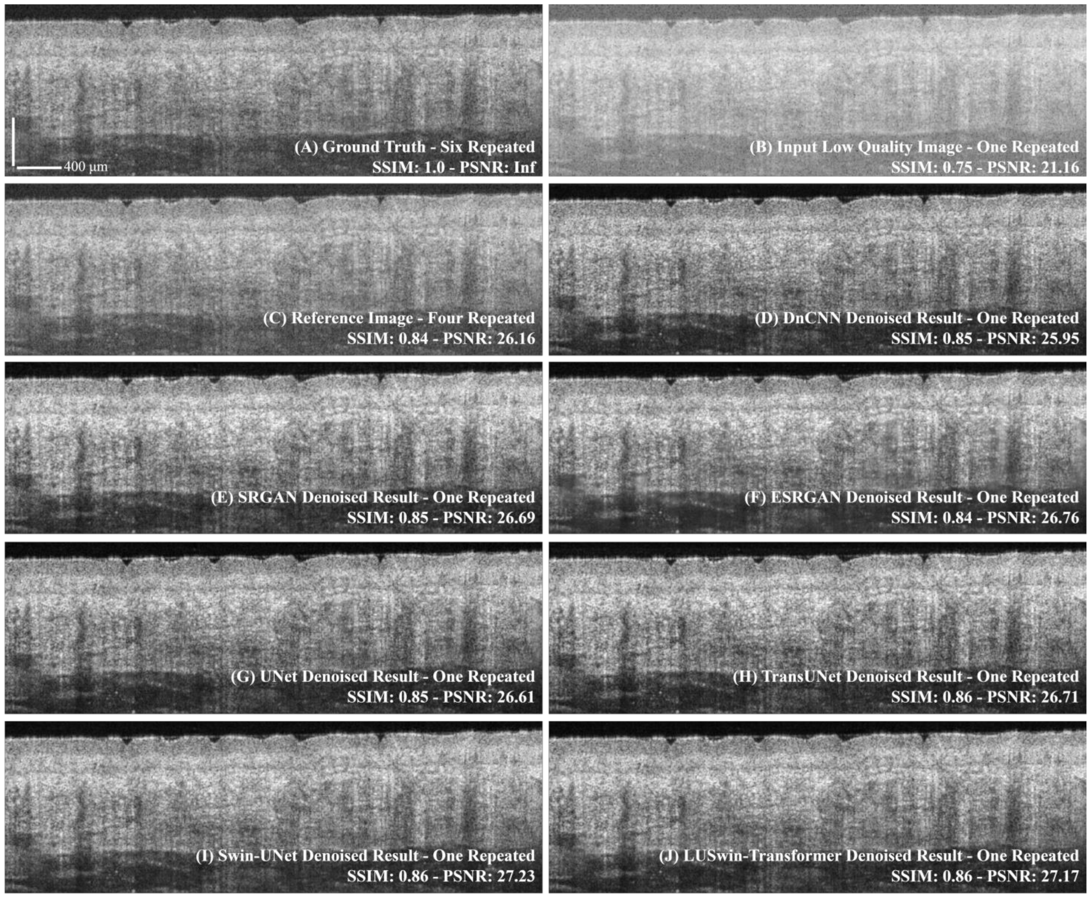
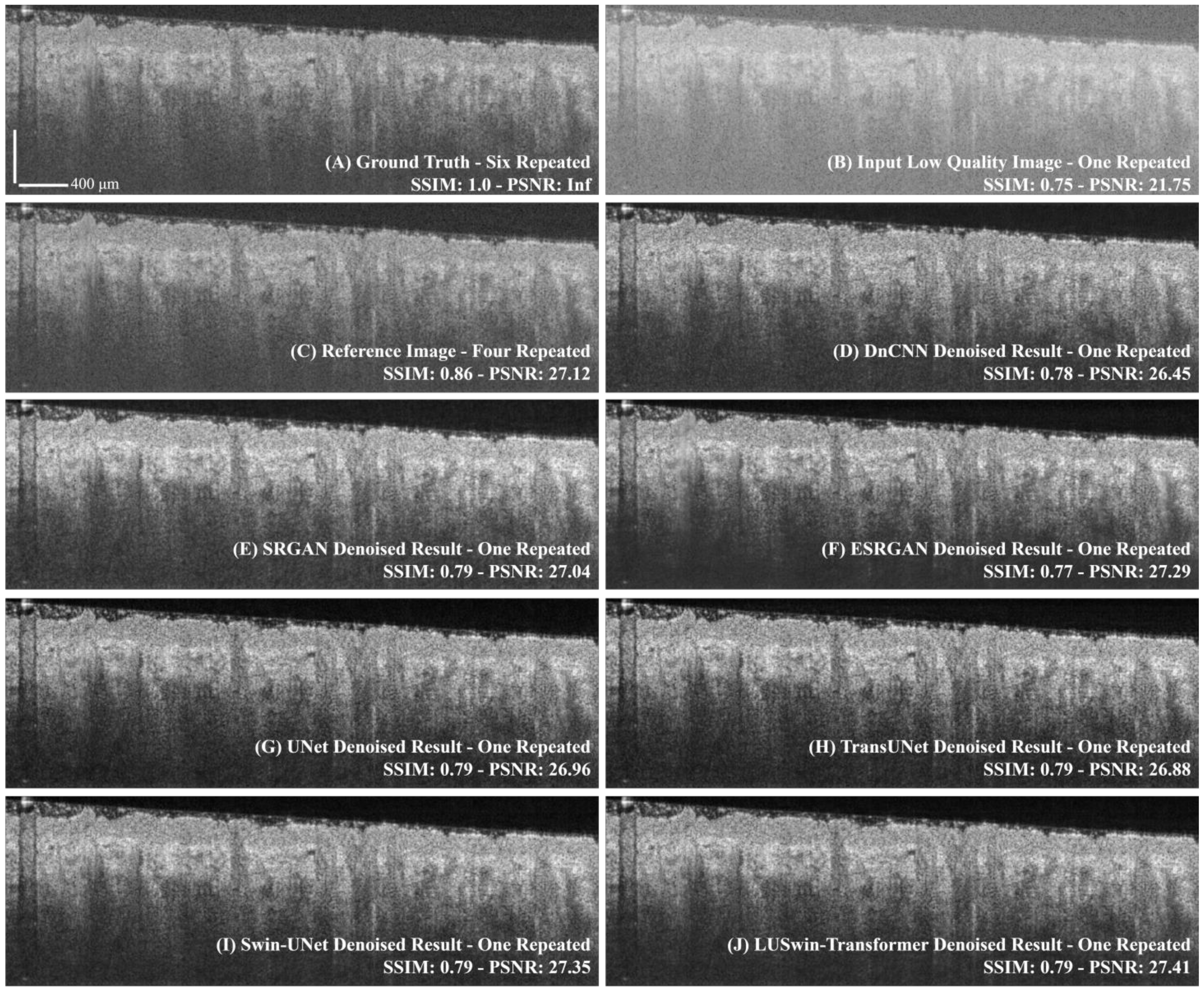
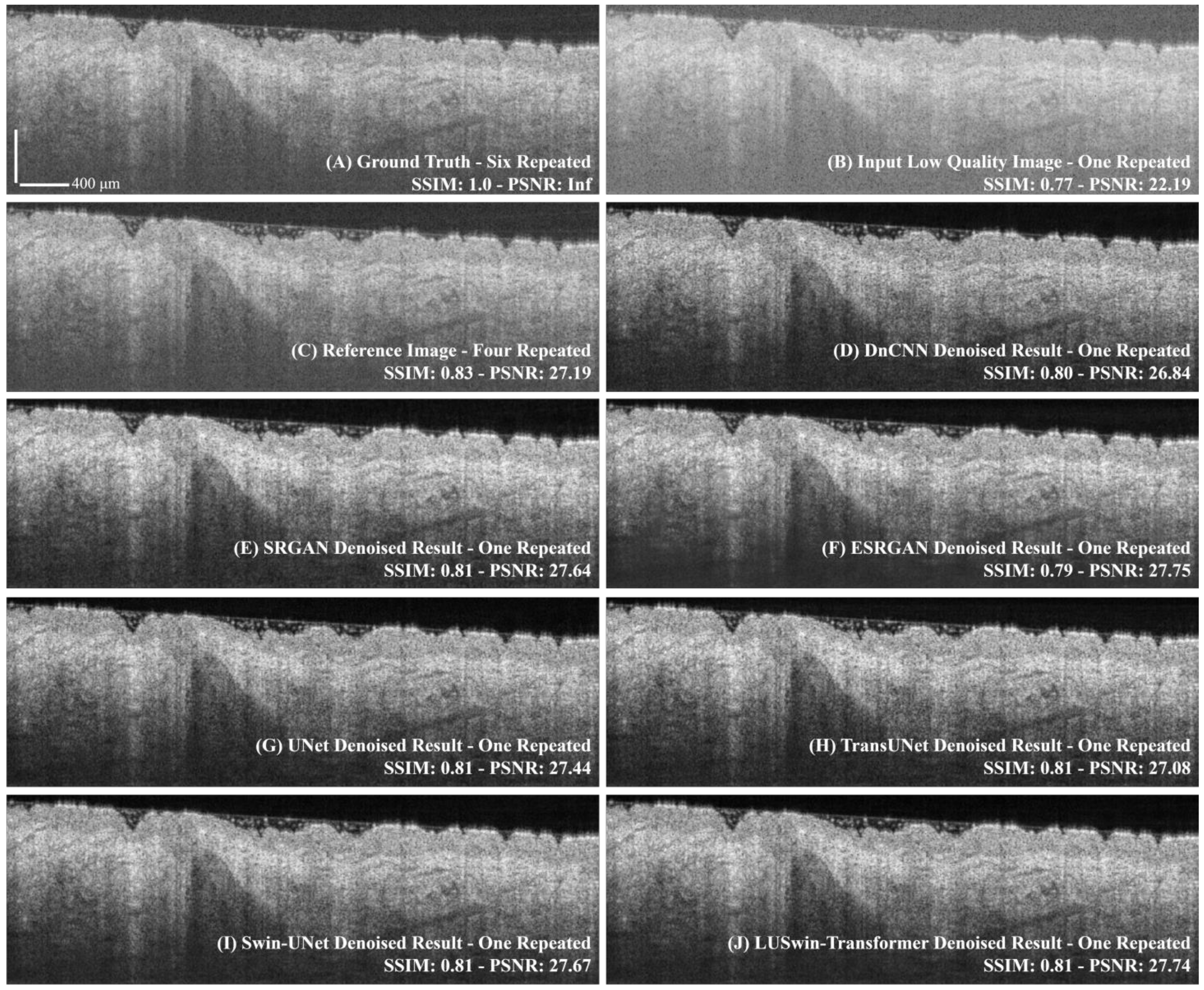
3.1. Comparison of the Different Networks

Table 3 demonstrates the quantitative comparison between the different methods. The floating-point operations (FLOPs) and network parameters (Params) are used to compare the computational cost of the networks. In the comparison of the results, except for the DnCNN, all the neural networks can provide better mean PSNR results than the baseline reference (mean PSNR: 26.19). Among them, Swin-UNet has the best PSNR (26.94) performance, but the difference with the LUSwin transformer (26.92) is slight, while the second best LUSwin transformer has the smallest FLOPs (3.9299 G), which is approximately three times smaller than Swin-UNet. Among the CNN-type networks that employ residual connections, SRGAN (mean PSNR: 26.42) and ESRGAN (mean PSNR: 26.45) outperform DnCNN (mean PSNR: 25.32) and achieve more competitive results. In contrast, UNet has a higher PSNR (26.73) result than ESRGAN, while the FLOPs (59.882 G) are significantly smaller than ESRGAN (FLOPs: 258.51 G). TransUNet has smaller FLOPs (23.014 G) than UNet and higher SSIM (0.796), but contrarily performs worse than UNet in PSNR (26.68) result. Nevertheless, the frame averaging method with a four-repeated scan has a higher SSIM (0.858) result compared to all the denoised images by neural networks.
Figure 4 is the visual comparison between different methods. After comparing the denoised images by networks with the ground truth (A) and reference (C), we observed that they exhibit higher contrast and fewer noises. We believe that this improvement is due to the use of the L 2 loss function, which is also supported by [35]. In terms of visual observation, the difference between the neural networks is slight; however, excluding the DnCNN, the denoised images from the networks have a higher PSNR than the reference image (C) (PSNR: 26.16). Among them, the result from Swin-UNet (I) is the best (PSNR: 27.23) and the LUSwin transformer (J) is the second-best (PSNR: 27.17). Nevertheless, the SSIM results from neural networks are lower than the reference (C) (SSIM: 0.89), which has a similar situation to the quantitative results in Table 3. Our supposition is the cause of the higher contrast in the denoised images by neural networks. Additionally, to present the robustness and advanced denoising performance of the LUSwin transformer, two alternative denoised B-frame results that represent two different scan positions (i.e., face and neck) are presented in Appendix Figure A1 and Figure A2.

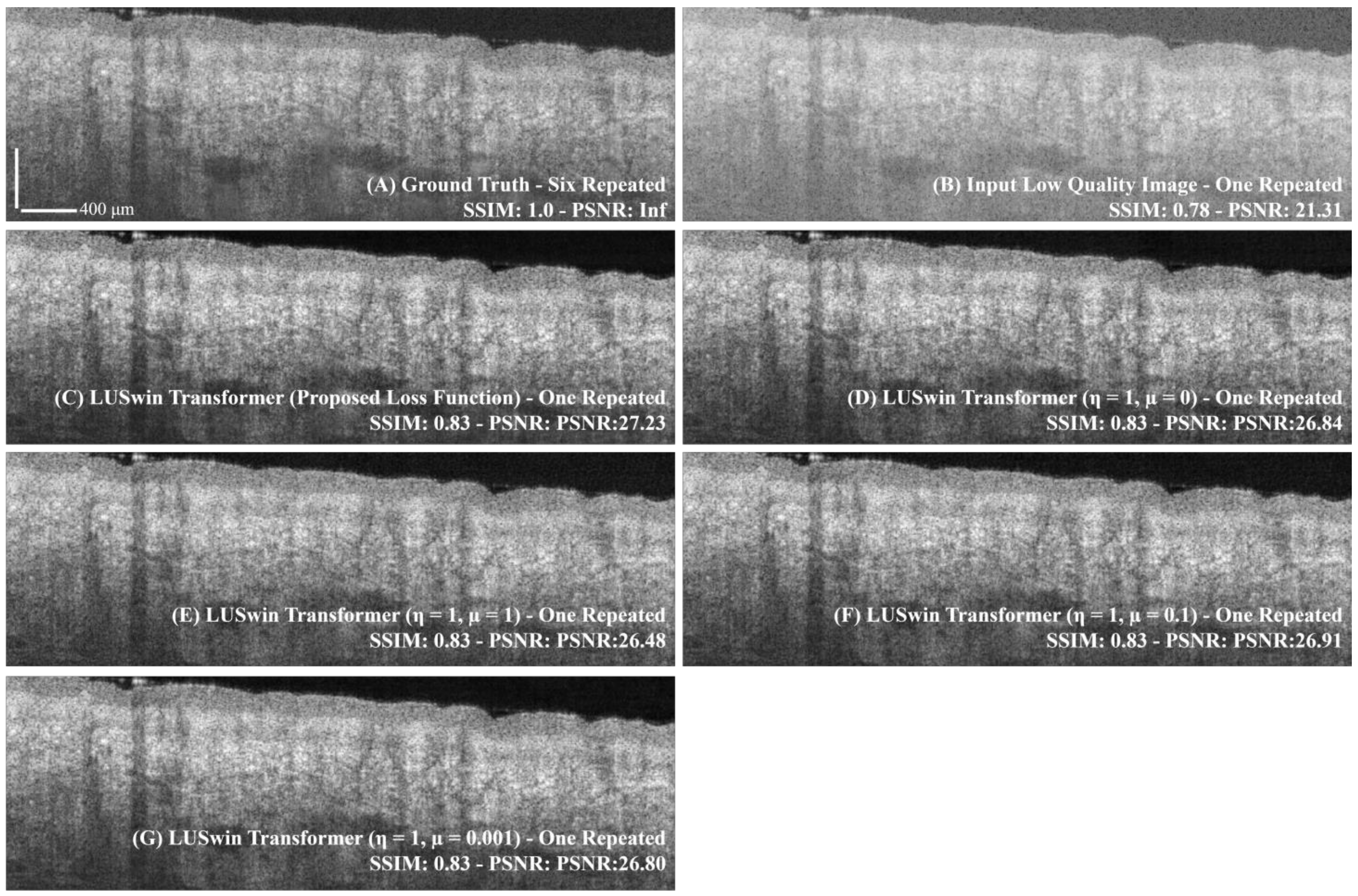
3.2. Comparison of the Different Loss Functions

Table 4 is a quantitative comparison of the LUSwin transformer trained under different loss functions. Compared with the L 2 -only result and other compared used setups of the L c loss function, the LUSwin transformer trained with the proposed L c has a higher mean PSNR (26.92) and SSIM (0.796) results. With respect to the visual comparison, in Figure 5, the proposed L c result (C) (PSNR: 27.23) and L c with μ   = 0.1 (F) (PSNR: 26.91) can provide less noise than the L 2 -only result (D) (PSNR: 26.84), while all of them have a higher contrast than the ground truth (A) and input (B).

3.3. Ablation Study Result

Table 5 presents a quantitative comparison between the proposed LUSwin transformer (control group) and its lighter variants, which employ different initialization parameters (i.e., the channel size) and architectures (i.e., the number of pairs of downsampled–upsampled blocks). The details of the experimental setup for each group can be found in Table 2, and the validation dataset is the same as mentioned in Table 3.
In the comparison of the results, the C-32 group demonstrates the lowest FLOPs (1.0447 G), but also the worst denoising performance (PSNR: 26.61; SSIM: 0.788). Both C-48 (PSNR: 26.72) and B-3 (PSNR: 26.61) groups exhibit similar performance, but the C-48 achieves a smaller FLOPs value (2.2561 G compared to 2.9267 G in B-3). Among them, the control group that utilizes the proposed implementation details achieved the best performance in terms of PSNR (26.77) and SSIM (0.792).

4. Discussion

In this study, we proposed a lightweight U-shape Swin (LUSwin) transformer to form an OCT image denoising pipeline for a fast one-repeated OCT scan in skin application. The results of the experiments demonstrate that the proposed LUSwin transformer has achieved a good denoising performance. Compared to the best performance Swin-UNet in this study, the LUSwin transformer has an approximately three times lower neural network size and FLOPs, while the degradation of the denoising performance is slight. In terms of network robustness and generalization, the LUSwin transformer has demonstrated that it can provide good denoising performance for noisy OCT images generated from five different scan positions (i.e., palm thenar, back of palm, forearm, face, and neck). Moreover, we introduced perceptual loss to improve the performance of the LUSwin transformer and enhance the training efficiency. Finally, the proposed LUSwin transformer has the lowest FLOPs among a series of state-of-the-art networks in image denoising, while providing advanced denoising performance.
Table 3 shows the quantitative comparison among the different methods, and most of the denoising networks improved the PSNR of the one-repeated noisy OCT image better than the four-repeated frame-averaging method, except the DnCNN. Of the denoising networks in this study, the proposed LUSwin transformer has the lowest computational cost as measured by FLOPs (3.9299 G), while achieving the second highest PSNR (26.92) and the highest SSIM (0.796). Regarding the utilization of the transformer, the comparison between the TransUNet (represents the pure transformer) and the LUSwin transformer (represents the Swin transformer) shows that the Swin transformer can enhance the denoising performance in terms of PSNR (26.92 > 26.68) while reducing the FLOPs (23.014 G > 3.9299 G) and network size (Parameters: 52.351 M > 11.922 M), and those advantages also exhibit in the comparison between Swin-UNet and TransUNet. Among the various CNN-type networks considered, UNet exhibits the highest PSNR (26.73) and SSIM (0.789). While SRGAN and ESRGAN have shown competitive performance in natural image super-resolution, our results demonstrate that in the denoising task, these methods underperform relative to UNet in regard to SSIM and PSNR. Our analysis suggests that the four-repeated frame averaging method exhibits limited performance in improving PSNR due to its calculation of the mean individual pixel intensity over the temporal frames, which preserves speckle information. Among the denoised results by the networks, TransUNet (SSIM: 0.796) and LUSwin transformer (SSIM: 0.796) have best improved the SSIM of the one-repeated noisy image. Nevertheless, the frame averaging method has a higher SSIM than all the denoised images by neural networks, and we hypothesize that this is because of the higher contrast in the network denoised images, as Figure 4D–J shows.
Figure 4 and Figure A1 and Figure A2 show that the B-frame images denoised by neural networks can improve contrast and noise reduction based on the input low-quality noisy image (B). We conjecture that this is because of the L 2 loss function, which is also supported by the results presented by Liu et al. [35]. Although the SSIM results of all the network-denoised images are lower than the reference (C), all of them can provide a higher contrast regarding the visual observations. Among them, the Swin-UNet (I) and LUSwin transformer (J) achieve the best quantitative results in terms of PSNR.
Table 4 and Figure 5 indicate that the introduced perceptual loss with the proposed implementation details can improve the denoising performance of the LUSwin transformer. Furthermore, our comparative study of the loss function ( L C ) recommends that the optimal perceptual loss weight is around 0.01. Since the weight is too large or too small (i.e., μ = 1 or μ = 0.001), it will decrease the denoising performance and training efficiency of neural networks. Although the training with the proposed loss function (i.e., L c ) requires an additional computation resource to output the feature maps from the VGG19 networks, which requires more time for training, the processing speed of the denoising operation is not influenced, and the utilization of the proposed L c is worthwhile.
Table 5 presents an ablation study that investigates the performance of the proposed LUSwin transformer when the network size is reduced. The comparison between different channel size setups indicates that decreasing the channel size (i.e., from 64 to 32) negatively impacts the denoising performance, with the PSNR dropping from 26.77 to 26.61. Moreover, reducing the number of downsampled–upsampled block pairs from 4 to 3 also leads to decreased denoising performance (PSNR from 26.77 to 26.71). In the comparison between the C-48 and B-3 results, reducing the channel size while maintaining the network depth (i.e., pairs of the downsampled–upsampled blocks) can provide a better denoising performance (PSNR: 26.72 > 26.71), while the FLOPs is smaller (2.2561 G < 2.9267 G). However, it is important to note that decreasing the neural network size of the LUSwin transformer can lead to a lower denoising performance. Consequently, we recommend using the LUSwin transformer with the proposed implementation details for optimal results in this study.
Our work has limitations in the training strategy. During the experiment stage, we found that the adversarial training for OCT image denoising will bring an unstable situation of network training and result in lower performance in the PSNR results. Although we investigated the strategies of relativistic average standard (RaS)-GAN [36], a label-smoothing method for discriminator, and Wasserstein GAN [37], the instability of the network training was not solved for encoder–decoder type networks (i.e., UNet, TransUNet, Swin-UNet, and LUSwin transformer). Therefore, we will investigate a more stable and higher efficiency method to introduce adversarial loss into the proposed LUSwin transformer and obtain a better competitive result in OCT image denoising.

5. Conclusions

In this study, we proposed an LUSwin transformer to build up an OCT image denoising pipeline for skin applications. The proposed LUSwin transformer achieved good competitive denoising results (PSNR: 26.92; SSIM:0.796) among different state-of-the-art networks while having a lightweight size design. In terms of network generalization and robustness, the denoising pipeline can perform stable denoising processing on five different positions of skin, representing different skin features. The proposed denoising pipeline can reduce the noise of the one-repeated noisy OCT images and improve the contrast and PSNR performance, which is useful for a fast OCT scan in skin applications.

Author Contributions

Conceptualization, J.L. and C.L.; methodology, software, validation, J.L.; formal analysis, J.L.; investigation, C.L.; resources, Z.H.; data curation, J.L., C.L. and Z.H.; writing—original draft preparation, J.L.; writing—review and editing, C.L. and Z.H.; visualization, J.L.; supervision, C.L. and Z.H.; project administration, C.L. and Z.H. All authors have read and agreed to the published version of the manuscript.

Funding

This research received no external funding.

Institutional Review Board Statement

The study was conducted in accordance with the Declaration of Helsinki and approved by the School of Science and Engineering Research Ethics Committee of the University of Dundee (code: UOD_SSREC_PGR_2022_003).

Informed Consent Statement

Informed consent was obtained from all subjects involved in the study. Written informed consent has been obtained from the patient(s) to publish this paper.

Data Availability Statement

The data presented in this study are available on request from the corresponding author. The data are not publicly available due to ethical restrictions.

Acknowledgments

The authors would like to express their gratitude to Tianyu Zhang, Yilong Zhang, Chunhui Li and Zhihong Huang for their support.

Conflicts of Interest

The authors declare no conflict of interest.

Appendix A

Figure A1. The visual comparison between the different methods. The image is selected from participant #011, representing the neural network performance on the face. (A) High-quality ground-truth image with six-repeated scans. (B) Low-quality input image with one-repeated scan. (C) High-quality reference image with four-repeated scans. (DJ) are neural networks denoised results from (D) DnCNN, (E) SRGAN, (F) ESRGAN, (G) UNet, (H) TransUNet, (I) Swin-UNet, and (J) LUSwin transformer. The white label is scale bar with 400 μm.
Photonics 10 00468 g0a1
Figure A2. The visual comparison between the different methods. The image is selected from participant #005, representing the neural network performance on the neck. (A) High-quality ground-truth image with six-repeated scans. (B) Low-quality input image with one-repeated scan. (C) High-quality reference image with four-repeated scans. (DJ) are neural networks denoised results from (D) DnCNN, (E) SRGAN, (F) ESRGAN, (G) UNet, (H) TransUNet, (I) Swin-UNet, and (J) LUSwin transformer. The white label is scale bar with 400 μm.
Photonics 10 00468 g0a2

References

  1. Honari, G. Skin structure and function. In Sensitive Skin Syndrome; CRC Press: Boca Raton, FL, USA, 2017; pp. 16–22. [Google Scholar]
  2. Fujimoto, J.W.; Drexler, G. Introduction to OCT. In Optical Coherence Tomography: Technology and Applications; Fujimoto, J.G., Drexler, W., Eds.; Springer International Publishing: Cham, Switzerland, 2015; pp. 3–64. [Google Scholar] [CrossRef]
  3. Levine, A.; Wang, K.; Markowitz, O. Optical coherence tomography in the diagnosis of skin cancer. Dermatol. Clin. 2017, 35, 465–488. [Google Scholar] [CrossRef]
  4. Mogensen, M.; Thrane, L.; Jørgensen, T.M.; Andersen, P.E.; Jemec, G.B.E. Optical coherence tomography for imaging of skin and skin diseases. In Seminars in Cutaneous Medicine and Surgery; WB Saunders: Philadelphia, PA, USA, 2009; pp. 196–202. [Google Scholar]
  5. Kollias, N.; Stamatas, G.N. Optical non-invasive approaches to diagnosis of skin diseases. In Journal of Investigative Dermatology Symposium Proceedings; Elsevier: Amsterdam, The Netherlands, 2002; pp. 64–75. [Google Scholar]
  6. Wang, Y.-J.; Wang, J.-Y.; Wu, Y.-H. Application of Cellular Resolution Full-Field Optical Coherence Tomography in vivo for the Diagnosis of Skin Tumours and Inflammatory Skin Diseases: A Pilot Study. Dermatology 2021, 238, 121–131. [Google Scholar] [CrossRef]
  7. Chen, I.-L.; Wang, Y.-J.; Chang, C.-C.; Wu, Y.-H.; Lu, C.-W.; Shen, J.-W.; Huang, L.; Lin, B.-S.; Chiang, H.-M. Computer-aided detection (CADe) system with optical coherent tomography for melanin morphology quantification in melasma patients. Diagnostics 2021, 11, 1498. [Google Scholar] [CrossRef]
  8. Wu, W.; Tan, O.; Pappuru, R.R.; Duan, H.; Huang, D. Assessment of frame-averaging algorithms in OCT image analysis. Ophthalmic Surg. Lasers Imaging Retin. 2013, 44, 168–175. [Google Scholar] [CrossRef] [PubMed]
  9. Liu, H.; Lin, S.; Ye, C.; Yu, D.; Qin, J.; An, L. Using a dual-tree complex wavelet transform for denoising an optical coherence tomography angiography blood vessel image. OSA Contin. 2020, 3, 2630–2645. [Google Scholar] [CrossRef]
  10. Huang, S.; Tang, C.; Xu, M.; Qiu, Y.; Lei, Z. BM3D-based total variation algorithm for speckle removal with structure-preserving in OCT images. Appl. Opt. 2019, 58, 6233–6243. [Google Scholar] [CrossRef] [PubMed]
  11. Bayhaqi, Y.A.; Hamidi, A.; Canbaz, F.; Navarini, A.A.; Cattin, P.C.; Zam, A. Deep-Learning-Based Fast Optical Coherence Tomography (OCT) Image Denoising for Smart Laser Osteotomy. IEEE Trans. Med. Imaging 2022, 41, 2615–2628. [Google Scholar] [CrossRef]
  12. Mehdizadeh, M.; MacNish, C.; Xiao, D.; Alonso-Caneiro, D.; Kugelman, J.; Bennamoun, M. Deep feature loss to denoise OCT images using deep neural networks. J. Biomed. Opt. 2021, 26, 046003. [Google Scholar] [CrossRef]
  13. Dong, Z.; Liu, G.; Ni, G.; Jerwick, J.; Duan, L.; Zhou, C. Optical coherence tomography image denoising using a generative adversarial network with speckle modulation. J. Biophotonics 2020, 13, e201960135. [Google Scholar] [CrossRef]
  14. Qiu, B.; You, Y.; Huang, Z.; Meng, X.; Jiang, Z.; Zhou, C.; Liu, G.; Yang, K.; Ren, Q.; Lu, Y. N2NSR-OCT: Simultaneous denoising and super-resolution in optical coherence tomography images using semisupervised deep learning. J. Biophotonics 2021, 14, e202000282. [Google Scholar] [CrossRef]
  15. Zhang, X.; Li, Z.; Nan, N.; Wang, X. Denoising algorithm of OCT images via sparse representation based on noise estimation and global dictionary. Opt. Express 2022, 30, 5788–5802. [Google Scholar] [CrossRef] [PubMed]
  16. Odena, A.; Dumoulin, V.; Olah, C. Deconvolution and checkerboard artifacts. Distill 2016, 1, e3. [Google Scholar] [CrossRef]
  17. Dosovitskiy, A.; Beyer, L.; Kolesnikov, A.; Weissenborn, D.; Zhai, X.; Unterthiner, T.; Dehghani, M.; Heigold, G.; Gelly, S.; Uszkoreit, J.; et al. An image is worth 16x16 words: Transformers for image recognition at scale. arXiv 2020, arXiv:2010.11929. [Google Scholar]
  18. Liu, Z.; Lin, Y.; Cao, Y.; Hu, H.; Wei, Y.; Zhang, Z.; Lin, S.; Guo, B. Swin transformer: Hierarchical vision transformer using shifted windows. In Proceedings of the IEEE/CVF International Conference on Computer Vision, Montreal, BC, Canada, 10–17 October 2021; pp. 10012–10022. [Google Scholar]
  19. Cao, H.; Wang, Y.; Chen, J.; Jiang, D.; Zhang, X.; Tian, Q.; Wang, M. Swin-unet: Unet-like pure transformer for medical image segmentation. arXiv 2021, arXiv:2105.05537. [Google Scholar]
  20. Ronneberger, O.; Fischer, P.; Brox, T. U-net: Convolutional networks for biomedical image segmentation. In International Conference on Medical Image Computing and Computer-Assisted Intervention; Springer: Berlin/Heidelberg, Germany, 2015; pp. 234–241. [Google Scholar]
  21. Zhang, T.; Zhou, K.; Rocliffe, H.R.; Pellicoro, A.; Cash, J.L.; Wang, W.; Wang, Z.; Li, C.; Huang, Z. Windowed Eigen-Decomposition Algorithm for Motion Artifact Reduction in Optical Coherence Tomography-Based Angiography. Appl. Sci. 2022, 13, 378. [Google Scholar] [CrossRef]
  22. Brash, D.E.; Ziegler, A.; Jonason, A.S.; Simon, J.A.; Kunala, S.; Leffell, D.J. Sunlight and sunburn in human skin cancer: p53, apoptosis, and tumor promotion. J. Investig. Dermatol. Symp. Proc. 1996, 1, 136–142. [Google Scholar]
  23. Cheng, Y.; Chu, Z.; Wang, R.K. Robust three-dimensional registration on optical coherence tomography angiography for speckle reduction and visualization. Quant. Imaging Med. Surg. 2021, 11, 879. [Google Scholar] [CrossRef]
  24. Klein, S.; Staring, M.; Murphy, K.; Viergever, M.A.; Pluim, J.P.W. Elastix: A toolbox for intensity-based medical image registration. IEEE Trans. Med. Imaging 2009, 29, 196–205. [Google Scholar] [CrossRef] [PubMed]
  25. Kingma, D.P.; Ba, J. Adam: A method for stochastic optimization. arXiv 2014, arXiv:1412.6980. [Google Scholar]
  26. He, K.; Zhang, X.; Ren, S.; Sun, J. Deep residual learning for image recognition. In Proceedings of the IEEE Conference on Computer Vision and Pattern Recognition, Las Vegas, NV, USA, 27–30 June 2016; pp. 770–778. [Google Scholar]
  27. Johnson, J.; Alahi, A.; Fei-Fei, L. Perceptual losses for real-time style transfer and super-resolution. In European Conference on Computer Vision; Springer: Berlin/Heidelberg, Germany, 2016; pp. 694–711. [Google Scholar]
  28. Ledig, C.; Theis, L.; Huszár, F.; Caballero, J.; Cunningham, A.; Acosta, A.; Aitken, A.; Tejani, A.; Totz, J.; Wang, Z.; et al. Photo-realistic single image super-resolution using a generative adversarial network. In Proceedings of the IEEE Conference on Computer Vision and Pattern Recognition, Honolulu, HI, USA, 21–26 July 2017; pp. 4681–4690. [Google Scholar]
  29. Wang, X.; Yu, K.; Wu, S.; Gu, J.; Liu, Y.; Dong, C.; Qiao, Y.; Loy, C.C. Esrgan: Enhanced super-resolution generative adversarial networks. In Proceedings of the European Conference on Computer Vision (ECCV), Munich, Germany, 8–14 September 2018; p. 0. [Google Scholar]
  30. Simonyan, K.; Zisserman, A. Very Deep Convolutional Networks for Large-Scale Image Recognition. arXiv 2014, arXiv:1409.1556. [Google Scholar]
  31. Abadi, M.; Barham, P.; Chen, J.; Chen, Z.; Davis, A.; Dean, J.; Devin, M.; Ghemawat, S.; Irving, G.; Isard, M.; et al. Tensorflow: A system for large-scale machine learning. In 12th {USENIX} Symposium on Operating Systems Design and Implementation ({OSDI} 16); USENIX: Berkely, CA, USA, 2016; pp. 265–283. [Google Scholar]
  32. Zhang, K.; Zuo, W.; Chen, Y.; Meng, D.; Zhang, L. Beyond a gaussian denoiser: Residual learning of deep cnn for image denoising. IEEE Trans. Image Process. 2017, 26, 3142–3155. [Google Scholar] [CrossRef] [PubMed]
  33. Chen, J.; Lu, Y.; Yu, Q.; Luo, X.; Adeli, E.; Wang, Y.; Lu, L.; Yuille, A.L.; Zhou, Y. Transunet: Transformers make strong encoders for medical image segmentation. arXiv 2021, arXiv:2102.04306. [Google Scholar]
  34. Wang, Z.; Bovik, A.C.; Sheikh, H.R.; Simoncelli, E.P. Image quality assessment: From error visibility to structural similarity. IEEE Trans. Image Process. 2004, 13, 600–612. [Google Scholar] [CrossRef] [PubMed]
  35. Liu, X.; Huang, Z.; Wang, Z.; Wen, C.; Jiang, Z.; Yu, Z.; Liu, J.; Liu, G.; Huang, X.; Maier, A.; et al. A deep learning based pipeline for optical coherence tomography angiography. J. Biophotonics 2019, 12, e201900008. [Google Scholar] [CrossRef]
  36. Jolicoeur-Martineau, A. The relativistic discriminator: A key element missing from standard GAN. arXiv 2018, arXiv:1807.00734. [Google Scholar]
  37. Arjovsky, M.; Chintala, S.; Bottou, L. Wasserstein generative adversarial networks. In Proceedings of the International Conference on Machine Learning, Sydney, NS, Australia, 6–11 August 2017; pp. 214–223. [Google Scholar]
Figure 1. The OCT structural image denoising pipeline including the training pipeline. The noisy structural image is generated based on the single OCT-scanned B-frame. The high-quality image is generated by the frame averaging method [8] with six-repeated OCT-scanned B-frames. In the training stage, the denoised image from the denoise network was used to calculate the loss for the neural network’s trainable weights updating. In the test stage, the denoised image is compared with the high-quality image to evaluate the performance of the denoise network based on validation sets.
Photonics 10 00468 g001
Figure 2. The system schematic of the swept-source (SS) OCT system in this study. The data acquisition card used in the personal computer (PC) is an ATS9371 from AlazarTechTM, and the sample lens in the system is an LSM03 from Thorlabs with a 35 mm focus length. (a) A demonstration of the data acquisition with a flexible hand-held scan probe, which is built-in in the SSOCT system.
Photonics 10 00468 g002
Figure 3. The architecture of the lightweight U-shape Swin transformer, which consists of an encoder (blue zone), bottleneck (organ zone), and decoder (red zone). W and H are the width and height of the image and feature map, respectively. C is the channel of the tensor, which is set to 64 in this study for the proposed LUSwin transformer. The bold dotted line between the encoder and decoder is a skip connection to provide residual learning and improve the training efficiency [26]. Patch merging is used to downsample the shape of the feature map, while the expanded layer is used to upsample the feature map. (a) The Swin transformer block (STB) used in the LUSwin transformer. (b) The demonstration of self-attention [17]. Q, K, and V are the sequences from the linear projection operation. In multi-head attention, Q, K, and V are split into multi-head and then sent into the self-attention layer. d is a parameter with a numerical value of 1 / d i m s   o f   Q , and the output of the rescale is Q × K T d i m s   o f   Q .
Photonics 10 00468 g003
Figure 4. The visual comparison between the different methods. The image is selected from participant #004, representing the neural network performance on the palm thenar. (A) High-quality ground-truth image with six-repeated scans. (B) Low-quality input image with one-repeated scan. (C) High-quality reference image with four-repeated scans. (DJ) are the neural networks’ denoised results from (D) DnCNN, (E) SRGAN, (F) ESRGAN, (G) UNet, (H) TransUNet, (I) Swin-UNet, and (J) LUSwin transformer. The white label is a scale bar with 400 μm.
Photonics 10 00468 g004
Figure 5. The visual comparison between the different utilization of the loss function. The image is selected from participant #014, representing the neural network performance on the palm thenar. (A) High-quality ground-truth image with six-repeated scans. (B) Low-quality input image with one-repeated scan. (C) The denoised output from the LUSwin transformer with the proposed loss function and implementation details ( η = 1, μ = 0.01). (D) The denoised output from the LUSwin transformer with L 2 -only loss function ( η = 1, μ = 0). (E) The denoised output from the LUSwin transformer with L c ( η = 1, μ = 1) loss function. (F) The denoised output from the LUSwin transformer with L c ( η = 1, μ = 0.1) loss function. (G) The denoised output from the LUSwin transformer with L c ( η = 1, μ = 0.001) loss function. The white label is a scale bar with 400 μm.
Photonics 10 00468 g005
Table 1. Selected six-repeated OCT signals from the participants and relative scan positions.
Participant IDScan PositionsNumber of DataBiological Sex
#001Palm Thenar1Male
#002Palm Thenar2Male
#003Forearm (Arm)2Female
Neck2
#004Palm Thenar1Female
#005Neck1Male
Face1
#006Palm Thenar2Male
#007Palm Thenar1Male
#008Back of Palm2Female
Forearm (Arm)2
#009Neck2Female
#010Face2Male
#011Face1Male
#012Palm Thenar2Male
#013Palm Thenar1Female
#014Palm Thenar1Female
Forearm (Arm)1
#015Palm Thenar1Male
#016Palm Thenar1Female
Table 2. Ablation study setup of the proposed LUSwin transformer.
ExperimentsChannel Size (C)Pairs of Downsample–Upsample Blocks
Control Group644
Channel-4848 *4
Channel-3232 *4
Block-3643 *
* The parameter marked in bold is the different setup from the control group.
Table 3. Quantitative comparison (average ± standard deviation) with different methods.
MethodTypeRepeat ScanFLOPs * (G)Params * (M)PSNRSSIM
Input ImageN/A1-RepeatedN/AN/A21.28 ± 1.090.746 ± 0.047
ReferenceN/A4-RepeatedN/AN/A26.19 ± 1.230.858 ± 0.035
DnCNN [32]CNN1-Repeated40.9240.55725.32 ± 0.010.787 ± 0.040
SRGAN [28]CNN41.6840.56726.42 ± 0.910.792 ± 0.038
ESRGAN [29]CNN258.513.50626.45 ± 1.150.765 ± 0.051
UNet [20]CNN59.88234.56526.73 ± 0.630.789 ± 0.044
TransUNet [33]Transformer23.01452.35126.68 ± 0.010.796 ± 0.037
Swin-UNet [19]Transformer16.11750.28326.94 ± 0.580.795 ± 0.040
LUSwin TransformerTransformer3.929911.92226.92 ± 0.700.796 ± 0.040
* FLOPs: Floating point operations, the amount of calculation in the network. Smaller FLOPs mean faster neural network processing speed. The FLOPs calculation in this study is based on an input shape of 192 × 192 × 1. * Params (M): Parameter of the neural networks (unit: million).
Table 4. Quantitative comparison of the loss function based on the LUSwin transformer.
Loss Function η μ PSNRSSIM
L 2   ( μ   =   0 ) 1026.77 ± 0.530.792 ± 0.04
L C   ( μ   =   1 ) 1126.35 ± 0.540.793 ± 0.04
L C   ( μ   =   0.1 ) 10.126.71 ± 0.560.794 ± 0.04
L C (proposed)10.0126.92 ± 0.700.796 ± 0.04
L C   ( μ   =   0.001 ) 10.00126.76 ± 0.480.792 ± 0.04
Table 5. Quantitative comparison of the different setups of the LUSwin transformer.
Experiments *FLOPs (G)Params (M)PSNRSSIM
Control Group3.929911.92226.77 ± 0.530.792 ± 0.04
Channel (C)-482.25616.72626.72 ± 0.570.791 ± 0.04
Channel (C)-321.04473.01326.61 ± 0.510.788 ± 0.04
Block (B)-32.92672.98526.71 ± 0.530.791 ± 0.04
* Experiments. As mentioned in Table 2, channel C represents the channel size in Figure 3, and block B represents the number of pairs of downsampled (blue)–upsampled (red) blocks in Figure 3. The name of the experiments is thereby written as C-48, C-32, and B-3 in the main text.
Disclaimer/Publisher’s Note: The statements, opinions and data contained in all publications are solely those of the individual author(s) and contributor(s) and not of MDPI and/or the editor(s). MDPI and/or the editor(s) disclaim responsibility for any injury to people or property resulting from any ideas, methods, instructions or products referred to in the content.

