1. Introduction
In recent years, research into the cavity optomechanical system [
1,
2] has received more attention as a crossover research area between quantum optics and nano science. Studies about the cavity optomechanical system include the ground state cooling of mechanical oscillators [
3,
4], parametric normal-mode splitting [
5,
6], the preparation of non-classical states [
7,
8,
9] and the slow light effect [
10,
11,
12]. In the process of studying the cavity optomechanical system, Agarwal and his co-workers found the optomechanically induced transparency (OMIT) [
13]. The optomechanically induced transparency was fairly similar to the electromagnetically induced transparency (EIT) [
14]. We know that the electromagnetically induced transparency is a quantum coherent phenomenon: when a probe field interacts resonantly with a three-level atomic system driven by a strong coupling field, due to the quantum coherent control from the strong coupling field, coupling transition can occur, producing a pair of dressed state transitions. This changes the transition of the probe field into two transitions and leads destructive interference to absorption. Finally, the three-level atomic medium completely takes on the transparency phenomena for the probe field. EIT has become a quantum-manipulation technology widely used to manipulate quantum coherent media, based on the technology of EIT, double Fano resonance in a plasmonic double-grating structure [
15], a plasmonic multilayer system [
16] and metamaterial-induced transparency [
17].
The theoretical scheme of OMIT was first proposed by Agarwal and Huang in 2010 in Ref. [
13], and their studies showed how the probe field became transparent in optomechanical systems driven by a strong coupling field. Through the driving of this strong field, the first harmonic was generated. The reason for transparency was the occurrence of the destructive interference between the probe field and the first harmonic. In the year when the theory of OMIT was proposed, it was experimentally realized by Kippenberg’s group [
18]. Since then, OMIT has been considered for some physical systems, such as: superconducting loop systems [
19]; Fabry–Perot optical cavities with semi-permeable film in the middle [
20]; cascaded multimode-cavity optomechanical systems [
21]; Bogoliubov mechanical modes [
22]; cavity optomechanical systems with Kerr effect [
23] and diamond optomechanical crystals [
24]. Jing’s group obtained the optomechanically induced transparency in parity–time-symmetric microresonators [
25]. Using the quantum manipulation of OMIT, the generation of second-order and higher-order sidebands in the cavity optomechanical system was reported [
26,
27,
28]. In addition to the OMIT for a single probe field, researchers investigated two-color, electromagnetically induced transparency in a hybrid optomechanical system [
29]. Alongside in-depth studies about OMIT, this quantum coherence phenomenon was extended to a micro-resonator, coupled with nanoparticles [
30] and a spinning resonator [
31]. Because of the extremely narrow transparency peak, OMIT has a wide range of applications in precision measurements [
32,
33].
The reason why the optomechanical system exhibits so many novel physical phenomena is due to the important role of quantum nonlinearity. By using the Duffing nonlinearity, Franco’s group investigated steady-state mechanical squeezing in an optomechanical system [
34]. Regarding the coupling of the mechanical oscillator with the cavity field, the general processing mode is to treat the mechanical oscillator as a harmonic oscillator, meaning the mechanical oscillator has harmonic oscillator potential which is a quadratic function relating to position. In this work, we assumed that the mechanical oscillator had an anharmonic potential that included a cubic term besides the quadratic term of position. We investigated the optomechanically induced transparency of the optomechanical system, under the condition of the existence of a cubic anharmonic potential. We discussed the absorption and the dispersion spectrum of the output probe field in the system, under different strengths of mechanical nonlinearity and different values of other parameters. We found that the peak of the absorption and the dispersion spectrum will be asymmetric and the window of OMIT will deviate from the resonance point when a cubic nonlinearity oscillator exists in a system.
Our theoretical studies are based on current experimental progress in the field of cavity optomechanics. In order to numerically simulate the OMIT, our selections of parameters come from some experimental data. The research content of this paper is divided into three parts. In
Section 2, we describe the physical model, give the Hamiltonian of the system, and obtain the steady-state expectation values of the system operators. Next, we explain how we calculated the quantum fluctuations of the operators and the steady conditions. Then, we explain how we obtained the response of the cavity optomechanical system to the probe field. In
Section 3, we discuss influences of cubic anharmonic potential and other parameters on the absorption and the dispersion spectrum of the output probe field in the system. We briefly draw a conclusion in
Section 4.
2. Physical Model and Methods
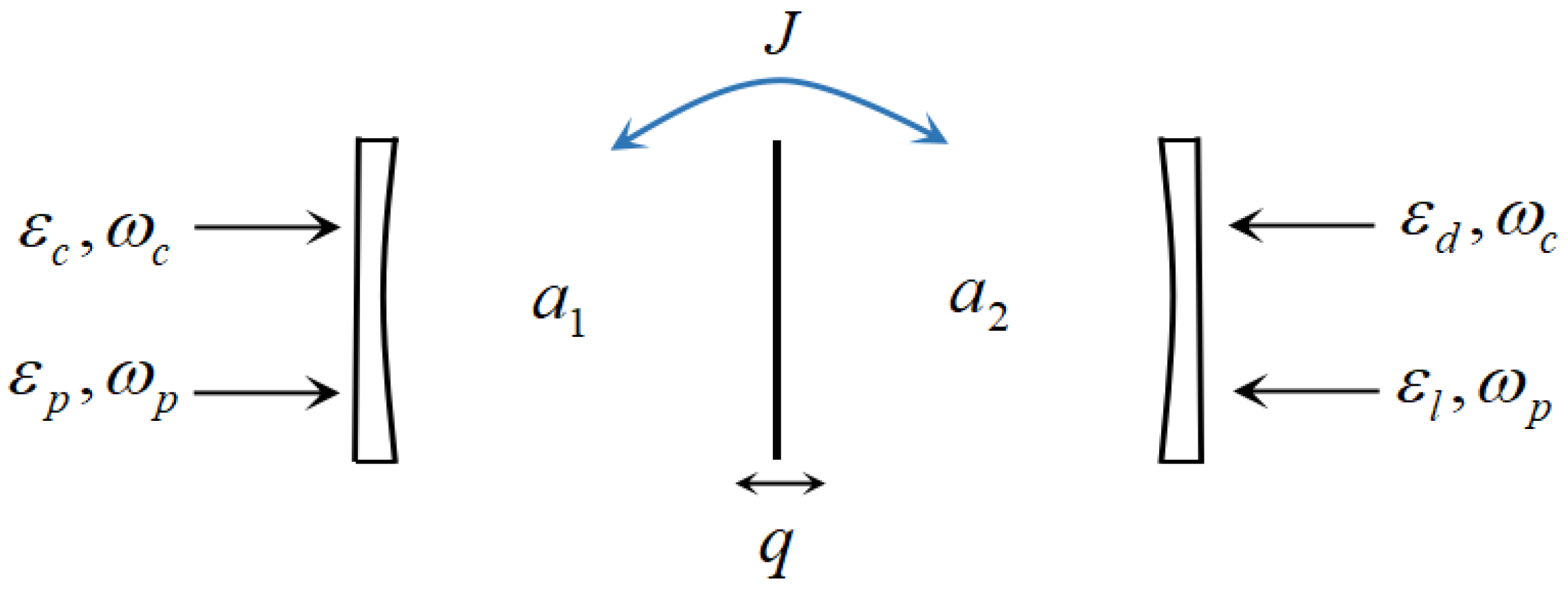
We considered a partially transparent membrane placed in the middle of a cavity. Due to the partial transmission and reflective property of the membrane, the membrane and the mirrors on the left and right sides of the cavity can form two cavities, respectively, as shown in
Figure 1. The membrane coupled with the two optical cavities simultaneously. When the cavities were driven by strong coupling fields, mechanical motion of the membrane occurred due to the radiation pressure force. In this system, we assumed that the membrane had potential that included harmonic oscillator potential, as well as anharmonic potential which related to the function of cubic of position. Here, the membrane was called a cubic anharmonic oscillator [
35], and it had nonlinear potential energy. In
Figure 1, two strong coupling fields (two weak probe fields) with the same frequency
ωc (the frequency
ωp of the two weak probe fields) and amplitudes
εc and
εd (the amplitudes
εp and
εl of the two weak probe fields) were used to drive cavity
a1 and
a2, respectively. This type of system has been studied on some phenomena in experiments [
36,
37,
38].
We describe the two optical cavities, respectively, by annihilation operators
ai and creation operators
while
are the resonance frequencies of the cavities and
are the decay rates of the cavities. The annihilation operators and creation operators are restricted by the commutation relation
. The mechanical oscillator, with a frequency
ωm and a damping rate
γm, is described by displacement operator
q and momentum operator
p. These two operators satisfy the relation
. The Hamiltonian of the cubic anharmonic oscillator is then given by
, where
m denotes the effective mass of the oscillator, and
α is the strength of the mechanical nonlinearity. Differences in
α lead to different coupling-constant behavior [
35]. It was found that the strength of the mechanical nonlinearity
α can be about 11 × 10
7 N/m
2 in a system containing a movable mirror and a cubic anharmonic oscillator [
39]. The first two terms in the above Hamiltonian represent the potential energy and kinetic energy of the harmonic oscillator, respectively, and the third term is the potential energy produced by the cubic mechanical nonlinearity. We write operators
p and
q as dimensionless momentum operator
P and displacement operator
Q.
P and
Q are defined by
and
, in which
is the amplitude of the zero-point motion of the mechanical oscillator and
is Planck constant.
P and
Q satisfy the relation
. Therefore, the Hamiltonian of the cubic anharmonic oscillator can be written as
,
. Since the cubic potential energy
is much smaller than the quadratic potential energy, we can think of the cubic potential energy as a perturbation. In the rotating-wave frame of coupling frequency
ωc, the total Hamiltonian of the optomechanical system can be written as:
Here, are the detuning between cavities and coupling fields, and is the detuning between probe fields and coupling fields. The first and the second terms are the energy of two cavities. The fourth and fifth terms represent the interaction between the mechanical oscillator and the two optical cavities, respectively, which was caused by radiation pressure with the coupling strength , with li being the length of cavities. The sixth term describes the Hamiltonian of the interaction between the two optical cavities. J is the coupling strength between the two cavities. The last four terms express the coupling of the coupling fields and the probe fields to the two optical cavities, respectively. The amplitudes of two coupling fields εd and εd are related to the decay rates κ1 and κ2 of the two optical cavity fields, the laser powers and and the frequency ωc of input fields, so they are described as and .
With the Hamiltonian written above in Equation (1), the dynamics of the system can be described by the quantum Langevin equation using the Heisenberg–Langevin equation:
Here,
is the input quantum vacuum noise in optical cavities with zero mean value
, and
is the nonzero time-domain correlation function, while
ξ is the thermal noise caused by the Brownian motion of the mechanical oscillator. The correlation function in the time domain is:
and its mean value is zero
. In the above equation,
kB is the Boltzmann constant and
T is the ambient temperature of the system. In this paper, we discuss the average response of the system to the input probe field; thus, the effect of the noise can be ignored in the subsequent calculations. Since the probe field, compared to the coupling field, is a weak field, the effect of the probe field can be regarded as a perturbation. Therefore, due to the perturbation effect of the probe field, each operator can be viewed as the sum of a steady-state mean value and small fluctuation, so we obtain
,
,
. The steady-state mean value is related to the input coupling field. In the absence of probe fields
εp and
εl, we can obtain the steady-state mean values of operators in the system:
With denoting the effective detuning between two cavities and coupling fields, respectively, giQs is the optomechanical coupling strength of the mechanical oscillator and the two cavities, respectively. It can be noticed from the above equations that the steady-state mean value of the mechanical oscillator Qs depends on the mechanical nonlinearity strength α and the number of cavity photons .
The quantum Langevin equations in Equation (2) are nonlinear equations, so we solve them by keeping the only linear terms of fluctuation operators and ignoring quadratic higher-order fluctuation. Therefore, the linearized quantum Langevin equations of fluctuation operators are shown as:
Due to the presence of the operators
, the amplitude and phase quadrature fluctuation operators of the cavities are introduced as
,
,
,
. The Langevin equations above in Equation (5) therefore can be written in the following matrix form:
where
f(
t),
fin and the coefficient matrix
M in Equation (6) are shown as follows:
Here,
,
,
,
,
,
,
,
. When the real parts of the eigenvalues of the coefficient matrix
M are negative, the system may be in a steady state. We can use the method of the Routh–Hurwitz stability criterion [
40] to derive the stability conditions for the system. In the following discussion, it is necessary to make reasonable choices and adjustments to ensure that the system is always in a steady state.
For simplicity of calculation, we assumed that the membrane was a perfect semi-transmissive and semi-reflective membrane, and we let the amplitudes of the two probe fields be equal, that is, we let
. This was under the assumption that it was reasonable to expand the fluctuation operators by the perturbation method, as the form
, where
. If we substitute the form of every operator into Equation (5), it can be solved as follows:
With further calculations, output fields for both cavities can be obtained from:
where
For studying the output fields of both two cavities, we needed to work out the output fields
and
, which can be obtained according to the input–output relation [
18]
. From the model, we found that the input fields were
and
. Therefore, the output fields of this system were written as Equation (11):
Meanwhile, we expanded the output fields into the form of
in the same way. Combined with the input–output relationship, the output response corresponding to the probe fields of the two cavities can be obtained as:
We characterized the properties of the output probe fields by quadrature of the fields
and
, where the real part represents the absorption property, and the imaginary part represents the dispersion property [
17].
3. Discussion and Results
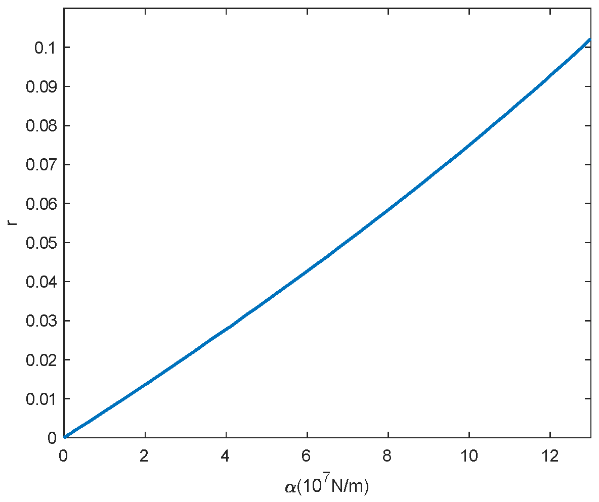
For this study, we first focused on the relationship between the ratio of the cubic potential energy to the quadratic potential energy of the mechanical oscillator and the mechanical nonlinearity strength
α. We assumed each coupling field drove cavities at the red-detuned mechanical sideband, making the effective detuning
and set
. Due to the steady condition, we referred to a study which has been worked out [
6], and the specific parameters were selected as follows: the frequencies of the input coupling fields are
GHz; the frequency of the mechanical oscillator is
MHz; the effective mass of the mechanical oscillator is
m = 12 pg; the coupling strength between the cavities and the mechanical oscillator is
Hz; the decay rate of the cavities is
; the damping rate of the mechanical oscillator is
Hz; the coupling strength between two cavities is
kHz and the power of the input coupling fields is
µw. It can be seen from Equations (9) and (10) that the output probe fields of the two cavities are the same under this set of parameters, which can be written as
.
Figure 2 shows the ratio of the cubic potential energy to the quadratic potential energy of the mechanical oscillator as a function of the mechanical nonlinearity strength
α. When the nonlinear strength
α increases from 0 to 12 × 10
7 N/m
2, the ratio of the cubic potential energy to the quadratic potential energy
increases as
α increases. When the mechanical nonlinearity strength reaches
α = 12 × 10
7 N/m
2, the ratio becomes
, which means the cubic potential energy is much smaller than the quadratic potential energy at steady state and can be regarded as a perturbation.
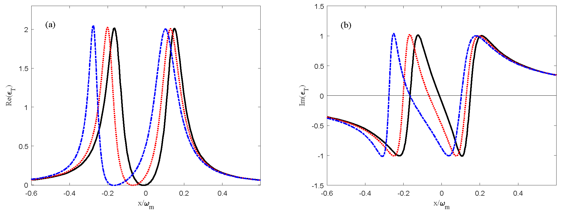
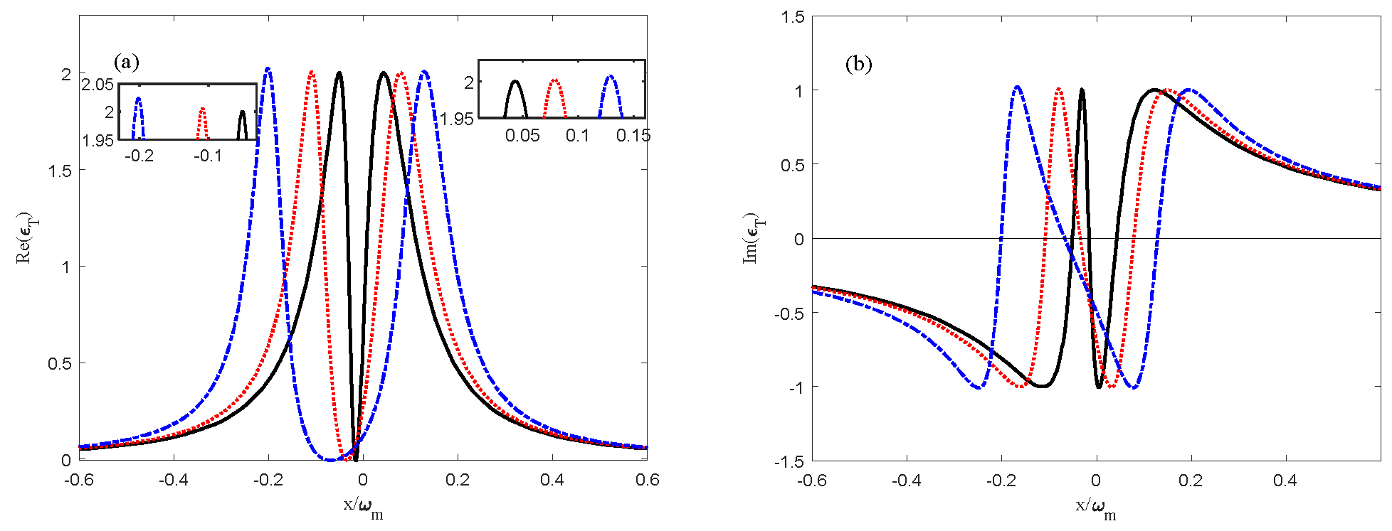
Next, we discuss the optomechanically induced transparency of the system containing a cubic anharmonic oscillator. We first considered the influence of the mechanical nonlinearity strength
α on the output probe field spectrum of the cubic potential energy contained in the mechanical oscillator. We plotted the real and the imaginary parts of the output field amplitude
εT versus the normalized frequency
x/
ωm for different mechanical nonlinearity strength
α = 0,
α = 5 × 10
7 N/m
2 and
α = 12 × 10
7 N/m
2. Here,
Figure 3a shows the real part of the output field amplitude
εT, and
Figure 3b shows the imaginary part of the output field amplitude
εT. As shown in
Figure 3a, there is a dip near
x = 0 where the detuning is
δ =
ωm as
α = 0. That is to say, the absorption effect of the optical system on the probe field is zero at the resonance when the mechanical nonlinearity strength is absent. The value of
εT is close to zero, and this means that the input probe field transmitted completely through the system without loss. With the increase in the mechanical nonlinearity strength, the two absorption peaks gradually become asymmetric; one absorption peak becomes higher and narrower, and the other absorption peak becomes lower and broader. At the same time, the positions of the two absorption peaks are shifted to the left, and the window width of the OMIT is slightly broader and is also shifted to the left and gradually deviated from the resonance point. The dispersion spectrum of the output field amplitude
εT is shown as
Figure 3b, and its slope represents the group delay. From the figure, we can see that as the mechanical nonlinearity strength increased, and the slope of the dispersion curve gradually decreased, which means the group delay became smaller near the point where the OMIT occurred.
Next, we discuss the differences between the spectrum of our OMIT and that of the standard OMIT in Ref. [
13]. In previous work [
13], the potential energy of a mechanical oscillator was
. In this case, when the oscillator was driven by the coupling field with frequency
ωc, it oscillated with the frequency
ωm, and the system generated harmonic wave with frequency
ωm +
ωc. If the
ωm +
ωc was equal to frequency
ωp of the probe field, interference phenomenon occured and the system could display a transparent window with two symmetrically distributed absorption peaks on both sides of the window, which is called the OMIT. However, in our paper, we considered that the membrane was in the potential energy with
+
which no longer represented a harmonic oscillator potential. The cubic anharmonic potential
changed the membrane’s oscillation frequency that was no longer equal to
ωm, so the position of the transparent window would shift, while the two absorption peaks were no longer strictly symmetrically changing the values of
α.
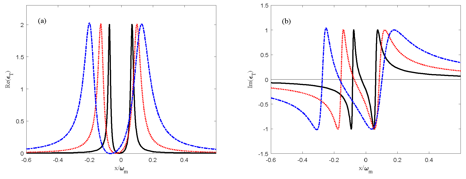
We plotted the output probe field amplitude
εT as a function of normalized detuning
x/
ωm for different decay rates
κ of the optical cavity field in
Figure 4. We chose the mechanical nonlinearity strength
α = 5 × 10
7 N/m
2 for the discussion of this part, and other parameters were the same as in
Figure 3. We focused on the corresponding output probe fields when the decay rates
κ were
κ = 0.02
ωm,
κ = 0.05
ωm and
κ = 0.1
ωm. It can be observed that the two absorption peaks became narrower gradually and had a slight tendency to become lower as the decay rate
κ became smaller and contracted towards the resonance point. The window width of OMIT became narrower, and the point where the OMIT appears shifted gradually to the right and closed towards the resonance point. In
Figure 4b, we find that the corresponding dispersion curve near the point where the absorption was zero became steeper as the decay rate decreased, and its slope increased as the decay rate decreased.
In addition to this, it can be seen that the coupling strength
g between the cavities and the oscillator, and the coupling strength
J between the two cavities are also factors affecting the output probe fields. In
Figure 5, we show the output probe field amplitude
εT as a function of normalized detuning
x/
ωm when the coupling strength
g between the cavities and the oscillator were
Hz,
Hz and
Hz. Mechanical nonlinearity strength
α = 5 × 10
7 N/m
2 was considered here, while the other parameters were the same as in
Figure 3. When the coupling strength
g became smaller, the two absorption peaks became lower and moved close to the resonance point, forming a narrower OMIT dip which also moved to the resonance point. The trend of the output probe field spectrum was similar to
Figure 4, but the reduction in
g could make the OMIT dip of the output field become narrower than in
Figure 4. The dispersion spectrum of the output probe field is plotted in
Figure 5b. We found that near the detuning corresponding to the OMIT dip, the slope of the curve became steeper as
g became smaller.
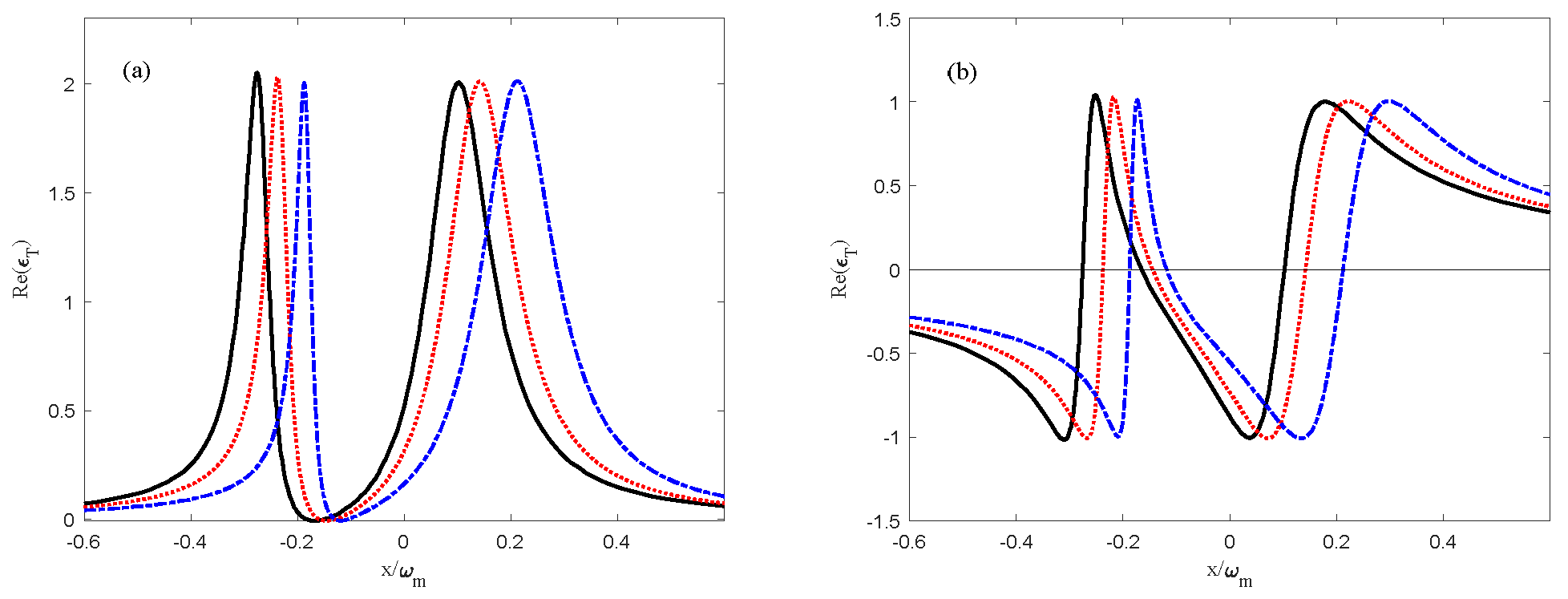
Finally, we discuss the influence of the coupling strength
J between the two cavities on output probe field
εT which is a function of normalized detuning
x/
ωm in
Figure 6. We chose the coupling strengths
kHz,
kHz and
kHz. When the coupling strength
J decreased, the two absorption peaks obviously became asymmetric. The absorption peak on the left became higher and wider and gradually moved away from the resonance point, while the absorption peak on the right became lower and narrower and moved towards the resonance point. Differing from the above discussion, the decrease in
J made the OMIT dip move towards to the left and away from the resonance point. In addition to this, the slope of the corresponding dispersion curve gradually became gentler as the coupling strength
J between the two cavities decreased.
4. Conclusions
Many phenomena have been achieved in the system with two cavities and an oscillator, such as coherent perfect absorption (CPA), coherent perfect transmission (CPT) and coherent perfect synthesis (CPS) [
41]. In this paper, we investigated the OMIT of the cavity optomechanical system containing a cubic anharmonic oscillator. We found that the presence of the cubic nonlinear anharmonic oscillator made the absorption spectrum of the output probe field become asymmetric and caused the OMIT dip to move away from the resonance point. These phenomena became stronger with the increase in the mechanical nonlinearity strength
α. Moreover, in the cavity optomechanical system with a cubic anharmonic oscillator, the decay rate of the cavity field, the coupling strength between the two optical cavities and the coupling strength between the cavities and the mechanical oscillator all affected the absorption peak of the output probe field and the position of the OMIT dip. Among these, a smaller decay rate of the cavity field, or a smaller coupling strength between the optical cavities and the mechanical oscillator led to a narrower OMIT dip, and the effective detuning where the OMIT occurred was closer to the resonance point
δ =
ωm. On the contrary, the effective detuning moved away from the resonance point
δ =
ωm where the OMIT occurred if the coupling strength between the two optical cavities decreased, even though the window width of OMIT was also slightly narrower. Besides this, the coupling strength between the two optical cavities also lead to a more obviously asymmetric phenomenon of the absorption peak, but it was opposite to the trend of the absorption peak height when the mechanical nonlinearity strength increased. Therefore, we found that we could adjust the position and width of the transparent window to achieve the OMIT required for different applications in this system. These results show that the influences of the cubic anharmonic potential on the spectrum of OMIT are significant, so we can detect the nonlinearity strength of the mechanical oscillator by measuring the shift of the transparent window. Our studies show the existence of cubic anharmonic potential to enhance the nonlinearity of the cavity optomechanical system; therefore, we can also extend this effect to the study of slow light and optical second-order sideband. Future research can also be extended to studying optomechanically induced amplification and optomechanically induced absorption, which provides optical information processing techniques for all-optical communication networks. Finally, we discuss the experimental feasibility of our scheme. With the development of micro/nano electromechanical technology, the optomechanical system has developed rapidly in recent years, and the parameters and scales of optomechanical systems have crossed the boundary between macro and micro. The oscillation frequency and effective mass values of the mechanical oscillator cover a very wide range, ranging from 10 to 10
9 Hz and from 10
3 to 10
−20 g, respectively. Electromagnetic radiation also spans the wavebands of microwaves and optical waves. In this paper, the frequencies of the input coupling fields were
GHz, the frequency of the mechanical oscillator was
MHz, and the effective mass of the mechanical oscillator was
m = 12 pg. Based on the current development of cavity optomechanical technology, maybe our scheme could be feasible for use in experiments.


