High-Quality Computational Ghost Imaging with a Conditional GAN


Abstract
:1. Introduction
2. Methods
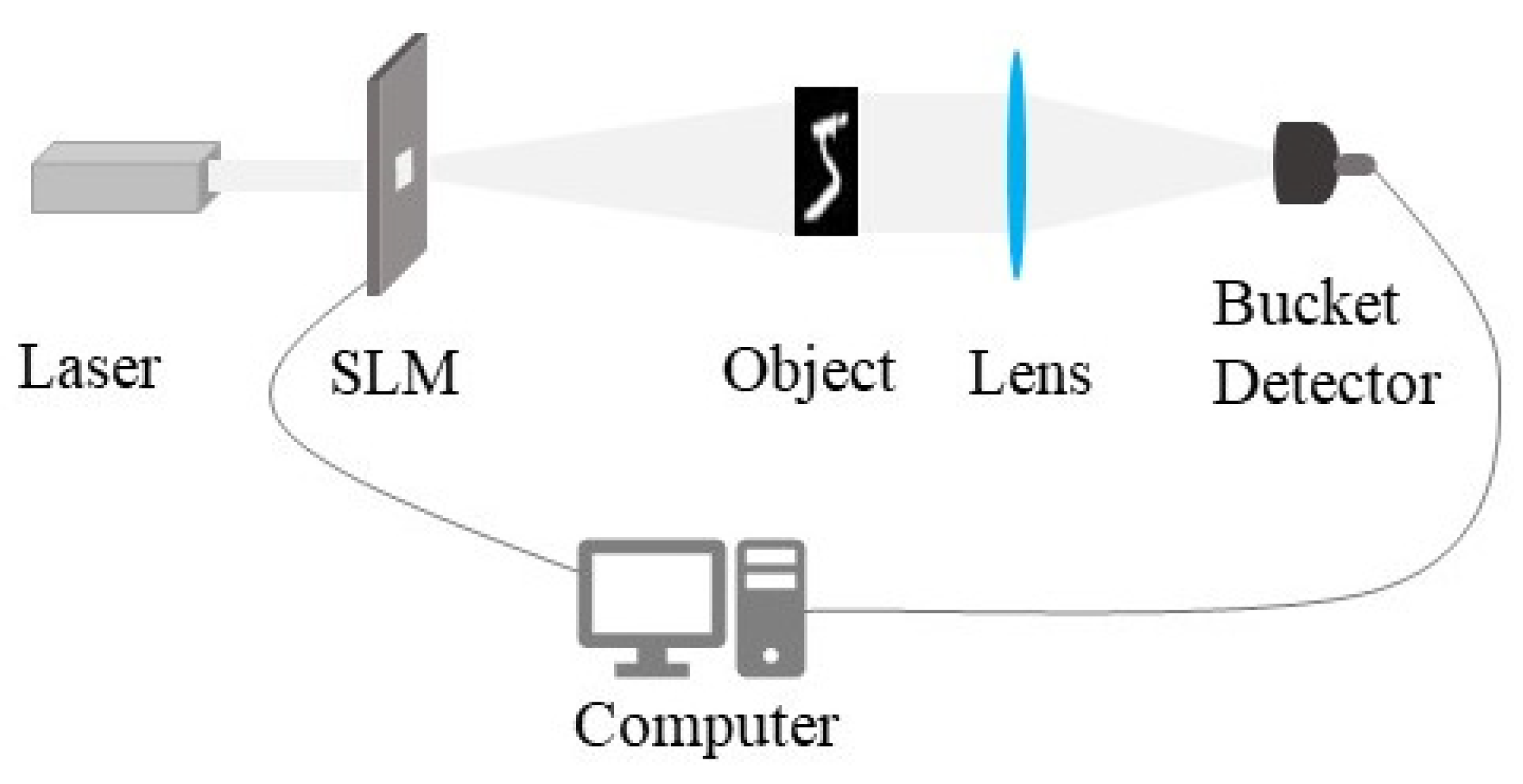
2.1. Imaging Scheme
2.2. Simulation
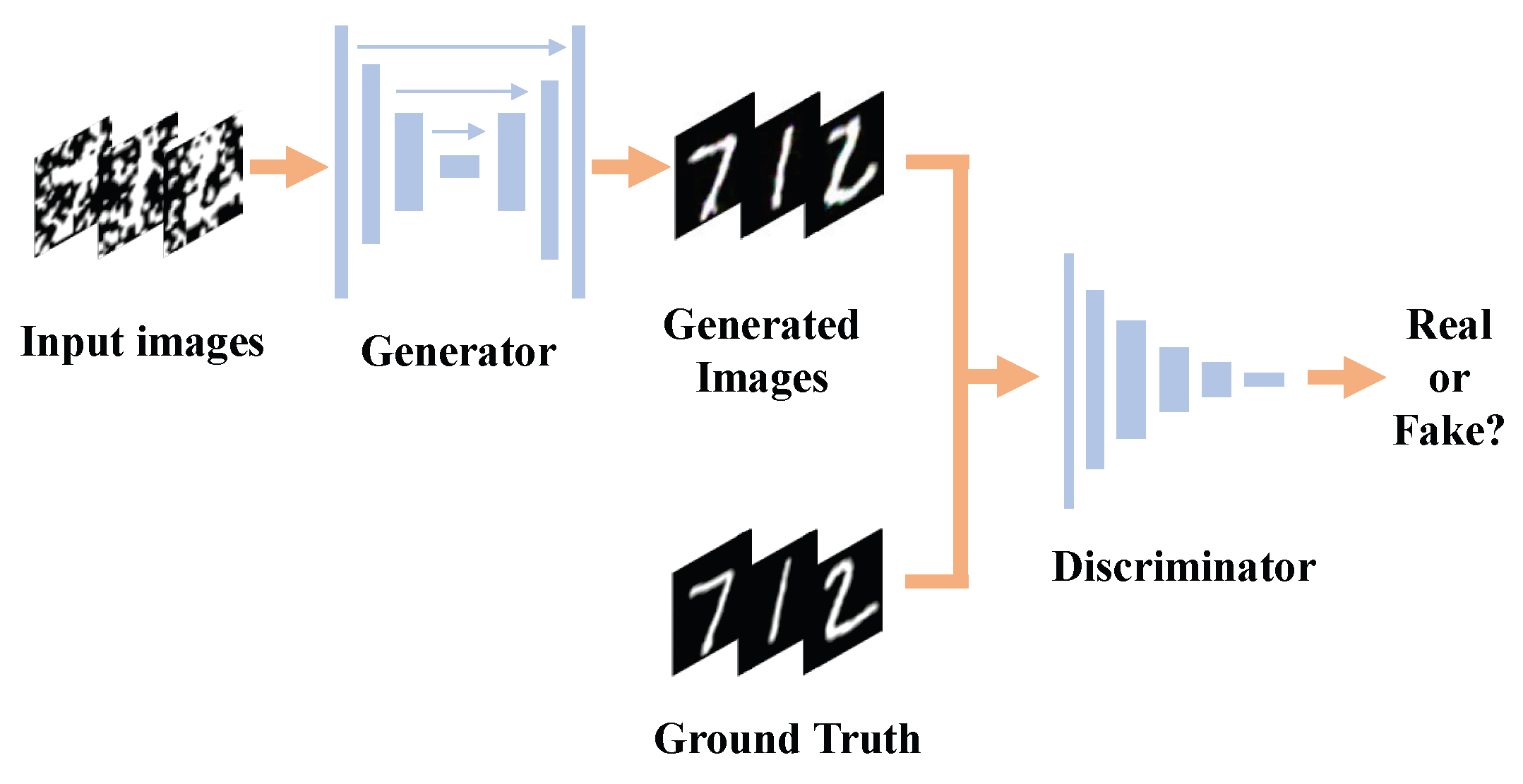
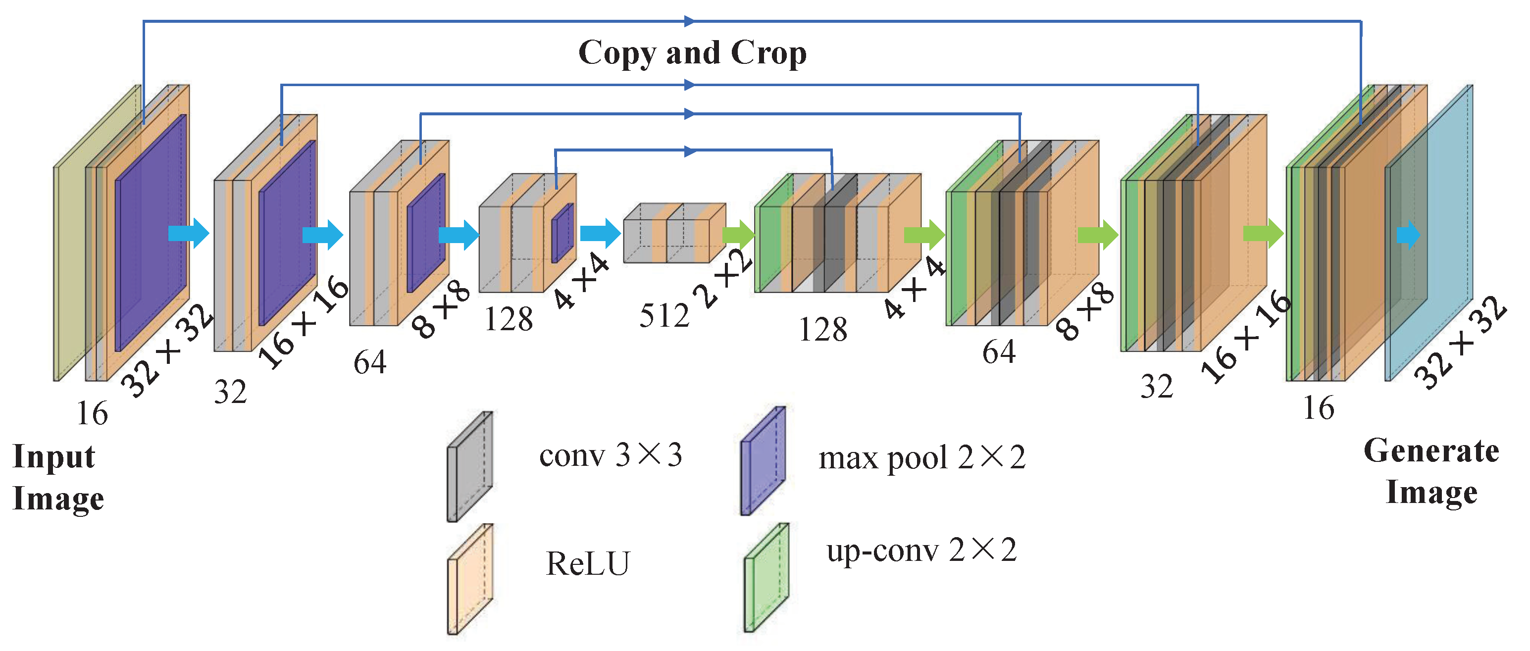
2.3. Network Structure
2.4. Preparation of Training Data and Network Training
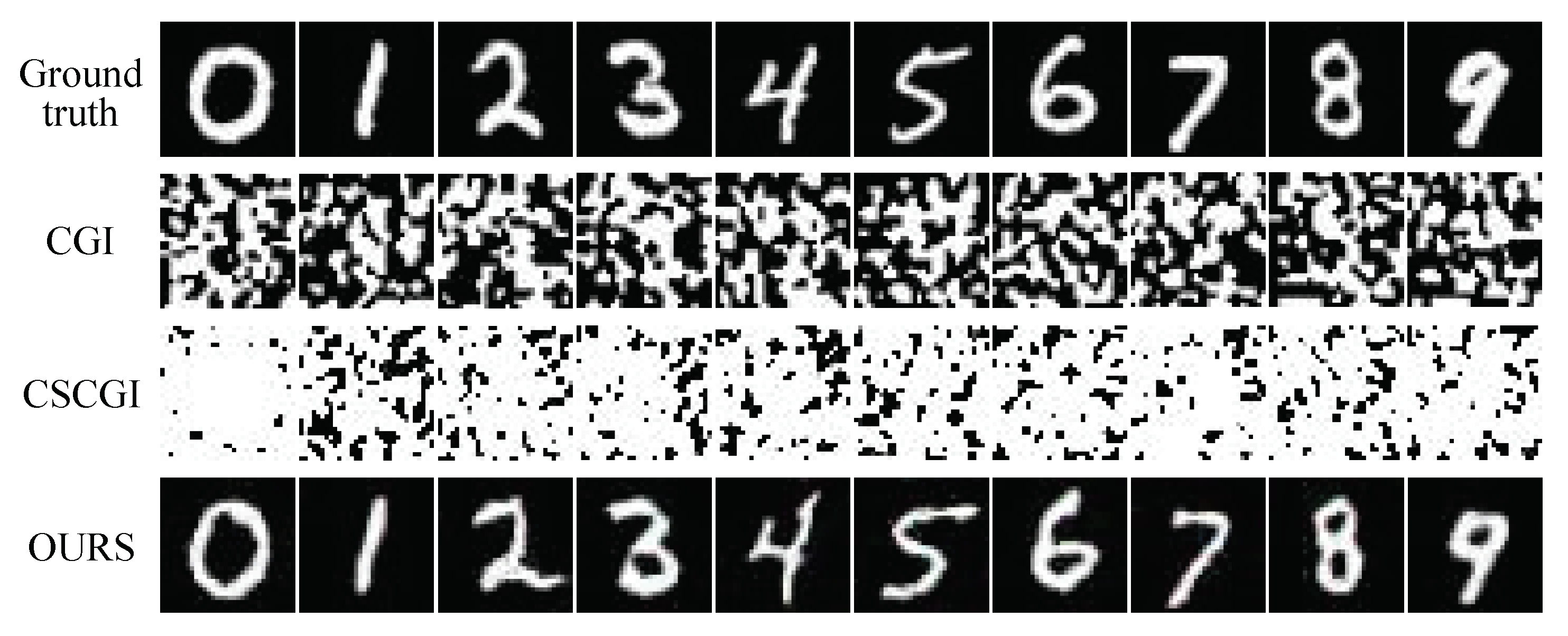
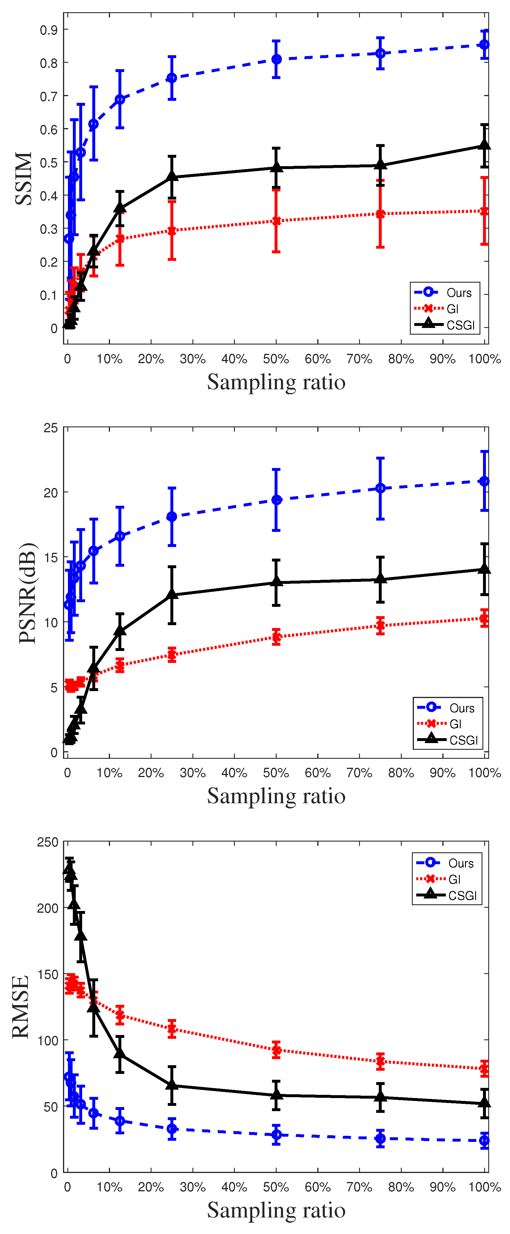
3. Results and Discussions
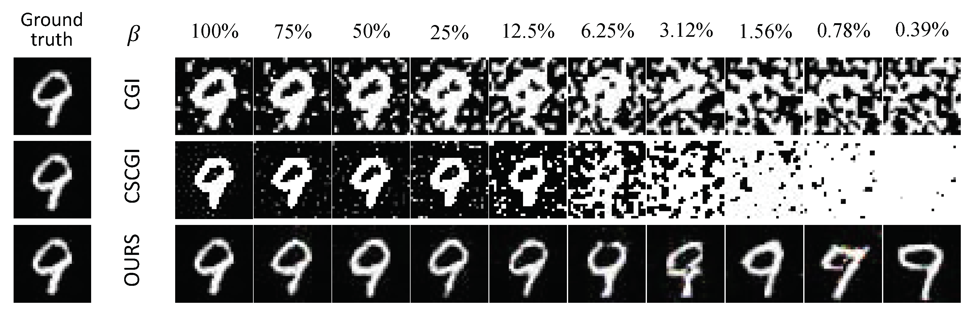
3.1. Results
3.2. Discussions
4. Conclusions
Author Contributions
Funding
Institutional Review Board Statement
Data Availability Statement
Acknowledgments
Conflicts of Interest
References
- Pittman, T.B.; Shih, Y.H.; Strekalov, D.V.; Sergienko, A.V. Optical imaging by means of two-photon quantum entanglement. Phys. Rev. A 1995, 52, R3429–R3432. [Google Scholar] [CrossRef]
- Shih, Y. Quantum Imaging. IEEE J. Sel. Top. Quantum Electron. 2007, 13, 1016–1030. [Google Scholar] [CrossRef]
- Shapiro, J.H.; Boyd, R.W. The physics of ghost imaging. Quantum Inf. Process. 2012, 11, 949–993. [Google Scholar] [CrossRef]
- Gatti, A.; Brambilla, E.; Bache, M.; Lugiato, L. Correlated imaging, quantum and classical. Phys. Rev. A 2003, 70, 235–238. [Google Scholar] [CrossRef] [Green Version]
- Cao, D.Z.; Xiong, J.; Wang, K. Geometrical optics in correlated imaging systems. Phys. Rev. A 2005, 71, 13801. [Google Scholar] [CrossRef] [Green Version]
- Zhang, P.; Gong, W.; Shen, X.; Han, S. Correlated imaging through atmospheric turbulence. Phys. Rev. A 2010, 82, 033817. [Google Scholar] [CrossRef] [Green Version]
- Shapiro, J.H. Computational Ghost Imaging. Phys. Rev. A 2008, 78, 061802. [Google Scholar] [CrossRef]
- Erkmen, B.I.; Shapiro, G.H. Ghost imaging: From quantum to classical to computational. Adv. Opt. Photonics 2010, 2, 405–450. [Google Scholar] [CrossRef]
- Ferri, F.; Magatti, D.; Lugiato, L.A.; Gatti, A. Differential Ghost Imaging. Phys. Rev. Lett. 2010, 104, 253603. [Google Scholar] [CrossRef] [Green Version]
- Sun, B.; Welsh, S.S.; Edgar, M.P.; Shapiro, J.H.; Padgett, M.J. Normalized ghost imaging. Opt. Express 2012, 20, 16892–16901. [Google Scholar] [CrossRef] [Green Version]
- Luo, K.H.; Huang, B.Q.; Zheng, W.M.; Wu, L.A. Nonlocal Imaging by Conditional Averaging of Random Reference Measurements. Chin. Phys. Lett. 2012, 29, 074216. [Google Scholar] [CrossRef] [Green Version]
- Gong, W.; Han, S. Correlated imaging in scattering media. Opt. Lett. 2011, 36, 394–396. [Google Scholar] [CrossRef] [Green Version]
- Yang, X.; Zhang, Y.; Xu, L.; Yang, C.H.; Wang, Q.; Liu, Y.-H.; Zhao, Y. Increasing the range accuracy of three-dimensional ghost imaging ladar using optimum slicing number method. Chin. Phys. B 2015, 24, 124202. [Google Scholar] [CrossRef]
- Ryczkowski, P.; Barbier, M.; Friberg, A.T.; Dudley, J.M.; Genty, G. Ghost imaging in the time domain. Nat. Photonics 2016, 10, 167–170. [Google Scholar] [CrossRef]
- Chen, X.; Jin, M.; Chen, H.; Wang, Y.; Qiu, P.; Cui, X.; Sun, B.; Tian, P. Computational temporal ghost imaging for long-distance underwater wireless optical communication. Opt. Lett. 2021, 46, 1938–1941. [Google Scholar] [CrossRef] [PubMed]
- Zhang, L.; Wang, Y.; Ye, H.; Xu, R.; Kang, Y.; Zhang, Z.; Zhang, D.; Wang, K. Camouflaged encryption mechanism based on sparse decomposition of principal component orthogonal basis and ghost imaging. Opt. Eng. 2021, 60, 013110. [Google Scholar] [CrossRef]
- Han, J.; Sun, L.; Lian, B.; Tang, Y. A deterministic matrix design method based on the difference set modulo subgroup for computational ghost imaging. IEEE Access 2021, 10, 66601–66610. [Google Scholar] [CrossRef]
- Zhao, H.; Wang, X.; Gao, C.; Yu, Z.; Wang, S.; Gou, L.; Yao, Z. Second-order cumulants ghost imaging. Chin. Opt. Lett. 2022, 20, 112602. [Google Scholar] [CrossRef]
- Bai, X.; Li, J.; Yu, Z.; Yang, Z.; Wang, Y.; Chen, X.; Yuan, S.; Zhou, X. Real single-channel color image encryption method based on computational ghost imaging. Laser Phys. Lett. 2022, 19, 125204. [Google Scholar] [CrossRef]
- Gao, Z.; Cheng, X.; Yue, J.; Hao, Q. Extendible ghost imaging with high reconstruction quality in strong scattering medium. Opt. Express 2022, 30, 45759–45775. [Google Scholar] [CrossRef]
- Lin, L.X.; Cao, J.; Zhou, D.; Hao, Q. Scattering medium-robust computational ghost imaging with random superimposed-speckle patterns. Opt. Commun. 2023, 529, 129083. [Google Scholar] [CrossRef]
- Cheng, J. Ghost imaging through turbulent atmosphere. Opt. Express 2009, 17, 7916–7921. [Google Scholar] [CrossRef] [PubMed]
- Gao, Z.; Cheng, X.; Chen, K.; Wang, A.; Hao, Q. Computational Ghost Imaging in Scattering Media Using Simulation-Based Deep Learning. IEEE Photonics J. 2020, 12, 1–15. [Google Scholar] [CrossRef]
- Zhao, C.; Gong, W.; Chen, M.; Li, E.; Wang, H.; Xu, W.; Han, A.S. Ghost imaging lidar via sparsity constraints. Appl. Phys. Lett. 2012, 101, 141123. [Google Scholar] [CrossRef] [Green Version]
- Chen, M.; Li, E.; Gong, W.; Bo, Z.; Xu, X.; Zhao, C.; Shen, X.; Xu, W.; Han, S. Ghost imaging lidar via sparsity constraints in real atmosphere. Opt. Photonic J. 2013, 3, 83–85. [Google Scholar] [CrossRef] [Green Version]
- Hardy, N.D.; Shapiro, J.H. Computational ghost imaging versus imaging laser radar for three-dimensional imaging. Phys. Rev. A 2013, 87, 023820. [Google Scholar] [CrossRef]
- Edgar, M.P.; Sun, B.; Bowman, R.; Welsh, S.S.; Padgett, M.J. 3D Computational Ghost Imaging. Int. Soc. Opt. Photonics 2013, 8899, 889902. [Google Scholar]
- Zhang, H.; Cao, J.; Zhou, D.; Cui, H.; Cheng, Y.; Hao, Q. Three-dimensional computational ghost imaging using a dynamic virtual projection unit generated by Risley prisms. Opt. Express 2022, 30, 39152–39161. [Google Scholar] [CrossRef]
- Ceddia, D.; Paganin, D.M. On Random-Matrix Bases, Ghost Imaging and X-ray Phase Contrast Computational Ghost Imaging. Phys. Rev. A 2018, 97, 062119. [Google Scholar] [CrossRef] [Green Version]
- Smith, T.A.; Shih, Y.; Wang, Z.; Li, X.; Adams, B.; Demarteau, M.; Wagner, R.; Xi, J.; Xia, L.; Zhu, R.Y. From optical to X-ray ghost imaging. Nucl. Instrum. Methods Phys. Res. Sect. A Accel. Spectrometers Detect. Assoc. Equip. 2019, 935, 173–177. [Google Scholar] [CrossRef] [Green Version]
- Yu, H.; Lu, R.; Han, S.; Xie, H.; Du, G.; Xiao, T.; Zhu, D. Fourier-Transform Ghost Imaging with Hard X Rays. Phys. Rev. Lett. 2016, 117, 113901. [Google Scholar] [CrossRef] [PubMed] [Green Version]
- Mizutani, Y.; Shibuya, K.; Iwata, T.; Takaya, Y. Fluorescence microscope by using computational ghost imaging. MATEC Web Conf. 2015, 32, 05001. [Google Scholar] [CrossRef] [Green Version]
- Yuan, S.; Wang, L.; Liu, X.; Zhou, X. Forgery attack on optical encryption based on computational ghost imaging. Opt. Lett. 2020, 45, 3917–3920. [Google Scholar] [CrossRef] [PubMed]
- Totero Gongora, J.S.; Olivieri, L.; Peters, L.; Tunesi, J.; Cecconi, V.; Cutrona, A.; Tucker, R.; Kumar, V.; Pasquazi, A.; Peccianti, M. Route to intelligent imaging reconstruction via terahertz nonlinear ghost imaging. Micromachines 2020, 11, 521. [Google Scholar] [CrossRef] [PubMed]
- Leibov, L.; Ismagilov, A.; Zalipaev, V.; Nasedkin, B.; Grachev, Y.; Petrov, N.; Tcypkin, A. Speckle patterns formed by broadband terahertz radiation and their applications for ghost imaging. Sci. Rep. 2021, 11, 20071. [Google Scholar] [CrossRef]
- Ismagilov, A.; Lappo-Danilevskaya, A.; Grachev, Y.; Nasedkin, B.; Zalipaev, V.; Petrov, N.V.; Tcypkin, A. Ghost imaging via spectral multiplexing in the broadband terahertz range. J. Opt. Soc. Am. B 2022, 39, 2335–2340. [Google Scholar] [CrossRef]
- Candes, E.J.; Romberg, J.; Tao, T. Robust uncertainty principles: Exact signal reconstruction from highly incomplete frequency information. IEEE Trans. Inf. Theory 2006, 52, 489–509. [Google Scholar] [CrossRef] [Green Version]
- Donoho, D.L. Compressed sensing. IEEE Trans. Inf. Theory 2006, 52, 1289–1306. [Google Scholar] [CrossRef]
- Katz, O.; Bromberg, Y.; Silberberg, Y. Compressive ghost imaging. Appl. Phys. Lett. 2009, 95, 131110. [Google Scholar] [CrossRef] [Green Version]
- Katkovnik, V.; Astola, J. Compressive sensing computational ghost imaging. J. Opt. Soc. Am. A 2012, 29, 1556–1567. [Google Scholar] [CrossRef] [Green Version]
- Du, J.; Gong, W.; Han, S. The influence of sparsity property of images on ghost imaging with thermal light. Opt. Lett. 2012, 37, 1067–1069. [Google Scholar] [CrossRef] [PubMed]
- Gong, W.; Han, S. Experimental investigation of the quality of lensless super-resolution ghost imaging via sparsity constraints. Phys. Lett. A 2012, 376, 1519–1522. [Google Scholar] [CrossRef] [Green Version]
- Chen, J.; Gong, W.; Han, S. Sub-Rayleigh ghost imaging via sparsity constraints based on a digital micro-mirror device. Phys. Lett. A 2013, 377, 1844–1847. [Google Scholar] [CrossRef]
- Sinha, A.T.; Lee, J.; Li, S.; Barbastathis, G. Lensless computational imaging through deep learning. Optica 2017, 4, 1117–1125. [Google Scholar] [CrossRef] [Green Version]
- Lyu, M.; Wang, W.; Wang, H.; Wang, H.; Li, G.; Chen, N.; Situ, G. Deep-learning-based ghost imaging. Sci. Rep. 2017, 7, 17865. [Google Scholar] [CrossRef] [Green Version]
- Shimobaba, T.; Endo, Y.; Nishitsuji, T.; Takahashi, T.; Nagahama, Y.; Hasegawa, S.; Sano, M.; Hirayama, R.; Kakue, T.; Shiraki, A.A. Computational ghost imaging using deep learning. Opt. Commun. 2017, 413, 147–151. [Google Scholar] [CrossRef] [Green Version]
- He, Y.; Wang, G.; Dong, G.; Zhu, S.; Chen, H.; Zhang, A.; Xu, Z. Ghost Imaging Based on Deep Learning. Sci. Rep. 2018, 8, 6469. [Google Scholar] [CrossRef] [PubMed] [Green Version]
- Zhang, C.; Zhou, J.; Tang, J.; Wu, F.; Cheng, H.; Wei, S. Deep unfolding for singular value decomposition compressed ghost imaging. Appl. Phys. B 2022, 128, 185. [Google Scholar] [CrossRef]
- Mirza, M.; Osindero, S. Conditional Generative Adversarial Nets. arXiv 2014, arXiv:1411.1784. [Google Scholar]
- Isola, P.; Zhu, J.; Zhou, T.; Efros, A.A. Image-to-Image Translation with Conditional Adversarial Networks. In Proceedings of the 2017 IEEE Conference on Computer Vision and Pattern Recognition (CVPR), Honolulu, HI, USA, 21–26 July 2017; pp. 5967–5976. [Google Scholar]
- Lecun, Y.; Bottou, L. Gradient-based learning applied to document recognition. Proc. IEEE 1998, 86, 2278–2324. [Google Scholar] [CrossRef] [Green Version]
- Bromberg, Y.; Katz, O.; Silberberg, Y. Ghost imaging with a single detector. Phys. Rev. A 2009, 79, 053840. [Google Scholar] [CrossRef] [Green Version]
- Katkovnik, V.; Astola, J.; Egiazarian, K. Discrete diffraction transform for propagation, reconstruction, and design of wavefield distributions. Appl. Opt. 2008, 47, 3481–3493. [Google Scholar] [CrossRef] [PubMed]
- Ronneberger, O.; Fischer, P.; Brox, T. U-Net: Convolutional Networks for Biomedical Image Segmentation. In Proceedings of the Medical Image Computing and Computer-Assisted Intervention-MICCAI 2015, Munich, Germany, 5–9 October 2015; pp. 234–241. [Google Scholar]
- Wang, Z.; Bovik, A.C.; Sheikh, H.R.; Simoncelli, E.P. Image Quality Assessment: From Error Visibility to Structural Similarity. IEEE Trans. Image Process. 2004, 13, 600–612. [Google Scholar] [CrossRef] [PubMed] [Green Version]


Disclaimer/Publisher’s Note: The statements, opinions and data contained in all publications are solely those of the individual author(s) and contributor(s) and not of MDPI and/or the editor(s). MDPI and/or the editor(s) disclaim responsibility for any injury to people or property resulting from any ideas, methods, instructions or products referred to in the content. |
© 2023 by the authors. Licensee MDPI, Basel, Switzerland. This article is an open access article distributed under the terms and conditions of the Creative Commons Attribution (CC BY) license (https://creativecommons.org/licenses/by/4.0/).
Share and Cite
Zhao, M.; Zhang, X.; Zhang, R. High-Quality Computational Ghost Imaging with a Conditional GAN. Photonics 2023, 10, 353. https://doi.org/10.3390/photonics10040353
Zhao M, Zhang X, Zhang R. High-Quality Computational Ghost Imaging with a Conditional GAN. Photonics. 2023; 10(4):353. https://doi.org/10.3390/photonics10040353
Chicago/Turabian StyleZhao, Ming, Xuedian Zhang, and Rongfu Zhang. 2023. "High-Quality Computational Ghost Imaging with a Conditional GAN" Photonics 10, no. 4: 353. https://doi.org/10.3390/photonics10040353