Article

Multiplane Image Restoration Using Multivariate Curve Resolution: An Alternative Approach to Deconvolution in Conventional Brightfield Microscopy

by
Sylvere Bienvenue Dion
1,*,
Don Jean François Ulrich Agre
1,
Akpa Marcel Agnero
1,2 and
Jérémie Thouakesseh Zoueu
1
1
Laboratoire d’Instrumentation Image et Spectroscopie (L2IS), Institut National Polytechnique Félix Houphouët-Boigny (INP-HB), Yamoussoukro BP 1093, Côte d’Ivoire
2
Département de Mathématiques-Physique-Chimie-Informatique, Université Jean Lorougnon Guédé, Daloa BP 150, Côte d’Ivoire
*
Author to whom correspondence should be addressed.
Photonics 2023, 10(2), 163; https://doi.org/10.3390/photonics10020163
Submission received: 10 November 2022 / Revised: 8 January 2023 / Accepted: 10 January 2023 / Published: 3 February 2023

Abstract

:
Three-dimensional reconstruction in brightfield microscopy is challenging since a 2D image includes from in-focus and out-of-focus light which removes the details of the specimen’s structures. To overcome this problem, many techniques exist, but these generally require an appropriate model of Point Spread Function (PSF). Here, we propose a new images restoration method based on the application of Multivariate Curve Resolution (MCR) algorithms to a stack of brightfield microscopy images to achieve 3D reconstruction without the need for PSF. The method is based on a statistical reconstruction approach using a self-modelling mixture analysis. The MCR-ALS (ALS for Alternating Least Square) algorithm under non-negativity constraints, Wiener, Richardson–Lucy, and blind deconvolution algorithms were applied to silica microbeads and red blood cells images. The MCR analysis produces restored images that show informative structures which are not noticeable in the initial images, and this demonstrates its capability for the multiplane reconstruction of the amplitude of 3D objects. In comparison with 3D deconvolution methods based on a set of No Reference Images Quality Metrics (NR-IQMs) that are Standard Deviation, ENTROPY Average Gradient, and Auto Correlation, our method presents better values of these metrics, showing that it can be used as an alternative to 3D deconvolution methods.

1. Introduction

The analysis of biological specimens requires, in many cases, for us to visualize their interior details. That has triggered research that implements optical sectioning. It is a powerful optical imaging technique which enables the three-dimensional (3D) reconstruction of the object and significantly improves the image contrast. Its implementation requires the recording of a stack of 2D images, which are taken at different z planes along the optical axis. Unfortunately, a 2D recorded image of a cell with a thickness that is greater than the depth of field of the microscope (as is the case of the most biological cells) results not only from the in-focus light, but also from the out-of-focus light. That leads to it completely to obscuring the in-focus details, and this greatly reduces the contrast of what remains. This is one of the major shortcomings in conventional optical microscopy. In addition, light which is out of focus is adversely affected by scatter, depending on the refractive index inhomogeneities, which are significantly present in biological tissue [1]. More light will appear to come from planes that are closer to the surface of the specimen than from those which are deeper inside of it [2]. This leads to the recording of a 2D image (which is a contribution of several sections of out-of-focus and in-focus light), where the details of the specimen’s structures have been removed [2,3,4,5]. Therefore, the 3D image is blurred. To remove this blurring, several techniques, either experimental or digital ones or both of them, have been proposed. The most common ones are Confocal Microscopy [2,6,7], Multiphoton microscopy [1,8] Structured Illumination Microscopy [5,9,10,11], Laser Sheet Microscopy [12,13], and Computational Optical Sectioning Microscopy (COSM) [3,4,14].
However, except for COSM, which employs a conventional brightfield microscope in the setup, the optical setups used in these advanced imaging techniques are complex and require a considerable data acquisition time and a considerable image post-processing time. In addition, the users need to be professionally trained to achieve image acquisition. The optical components required for these techniques increase the cost of the system. Therefore, a high-performance optical sectioning technique is at the expense of having a complex setup and its cost, which are factors that limits its combination with other systems, for example, robotic manipulation systems [15]. Thus, COSM is presented as an alternative approach to achieve brightfield optical sectioning [2,16]. This optical sectioning technique, generally, is linked to fluorescence microscopy, where photodamage and phototoxicity issues have been noted [17,18]. Adopting conventional brightfield microscopy for optical sectioning is of great significance because some of the biological specimens are not suitable for fluorescence imaging, it offers label-free imaging modalities, and it is simple, fast, and has a low cost. However, the technique has a poor optical sectioning ability [19,20]. Therefore, it is achieved using the computational deconvolution, which requires an accurate Point Spread Function (PSF). Modelling an accurate PSF is challenging, especially for conventional brightfield microscopy where the absorption and phase properties of the object must be considered [19,21]. The deconvolution in this case is not linear. A linear deconvolution can be considered in the case of purely phase or purely absorbing objects by neglecting the absorption part or phase part [19,21,22,23] by approximating the brightfield PSF [24] or by experimentally estimating the brightfield PSF [14]. Techniques using PSF models are becoming increasingly efficient [25], however, based on linear deconvolution, they can lead to approximate results or are not suitable for absorption and phase samples, such as biological cells with any properties of absorption.
In this study, we present a multiplane image restoration method. It is an alternative to computational deconvolution in brightfield microscopy that is based on the Multivariate Curve Resolution (MCR) analysis of z-scanning images taken with conventional brightfield microscopy. In addition to its speed, the simplicity, and the low cost of its setup, the technique is of great significance because of its implementation without the need for PSF and a priori knowledge of the samples. Efforts have recently been made in this direction in terms of the development of spatially incoherent annular illumination microscopy (SAIM) [20] and Optical Sectioning in Brightfield Microscopy (OSBM) [26]. However, SAIM requires us to modify the illumination, and OSBM is adapted for the phase samples. Our technique does not modify the conventional brightfield microscopy setup, and it is suitable for samples with light-absorbing properties. It uses transmittance images obtained using brightfield microscopy in transillumination. A 3D specimen with a thickness that is greater than the depth of field of the imaging system can be considered as a series of thin slices along the optical axis. The contributions of these thin slices are mixed in the image recorded. Here, a relationship between such an image and these thin slices is clearly derived from Beer–Lambert law. MCR, which is a self-modelling mixture analysis approach that was initially based on the multicomponent Beer–Lambert law, is used here to unmix the contributions of theses slices. The goal of this study is therefore to describe an alternative to deconvolution in conventional brightfield microscopy. Our technique was evaluated by making a comparison with it to the computational deconvolution microscopy methods.
The paper is organized as follows. Firstly, a background on deconvolution and MCR is given, which is followed by the methodology, which includes the experiments and the description of the way that the brightfield images are processed using MCR. The results are then presented and discussed.

2. Background and Related Work

2.1. Deconvolution

Deconvolution is an image restoration method which partially resolves the brightfield microscopy image distortion problem due to the imaging system limitations summarized in the 3D PSF and noise [4,14,27,28,29,30]. It is based on an image formation model that is defined by Equation (1). The goal is to approximate the intensity distribution f x , y , which is the ideal image that would be obtained if the imaging system had no defects, from the measurement g x , y and the PSF h x , y by considering the convolution model that is defined by Equation (1).
g x , y = f x , y h x , y + n x , y
where denote the convolution product and n x , y the noise term. In this paper, the described method is compared to the deconvolution methods such as Wiener filtering [27,28], Richardson–Lucy [27,31], and blind deconvolution [27,29]. Deconvolution is performed as described in [22], and the PSF used is the one developed by Aguet and Van de Ville [32], which is a version of the Gibson and Lanni theoretical PSF [33], with a few parameters.

2.2. Multivariate Curve Resolution

MCR is a set of high-performance statistical resolution methods, which allows for us to simultaneously extract the sample 𝐷, the spectra 𝑆 of the pure components, and their cartographies 𝐶 (concentrations profile) without any prior knowledge. They are thus meant to solve the mixture analysis problem based on the equation set by the multicomponent Beer–Lambert law [34,35,36,37]. The MCR analysis describes data according to the bilinear additive model given by Equation (2).
D = C S T + E
where E corresponds to the noise and errors matrix. The MCR method can therefore be applied to any data which can be effectively described by a bilinear equation model. However, the two ways of using the bilinear model must have clear meanings for this data system [35].
MCR, which was first designed for the analysis of single-order data matrices [38], has been then used to analyze multiway data matrices [39]. These kinds of data matrices including more than one matrix can be structured as a row-wise augmented matrix, a column-wise augmented matrix, or row and column-wise augmented matrices. The augmented matrices, which are also called multisets, are obtained according to the data structure. For spectroscopic imaging, the experimental data are a cube with x and y as the pixels number along two directions and n λ spectral channels number along the third direction. The cube is unfolded to obtain the matrix with x × y rows and n λ columns, to which the MCR algorithms are applied [40]. Note that a z-scanning brightfield optical microscope data set is analogous to the spectroscopic imaging data set with the difference that instead of having the number of spectral channels for the third direction, we have the number of planes in z direction along the optical axis.
The goal of MCR algorithms is to provide, following a bilinear model, the spectra and concentrations of pure species from a mixed original data table. For this work, an MCR-ALS (Multivariate Curve Resolution—Alternating Least Square) algorithm was used, it is freely available at: http://mcrals.info/ in MATLAB toolbox version. MCR-ALS is an iterative method that works by optimizing the initial estimates in an alternating least-squares way within each iterative cycle under the action of suitable constraints until the convergence criterion is fulfilled [35]. The initial estimates are based on the pure variable selection methods [41]. The constraints are mathematical conditions which are specific to the model of the measured data, which enable us to optimize the final solutions. The constraints commonly employed include non-negativity, unimodality, closure, equality, selectivity, species correspondence, model constraints, hard modelling, correlation constraints, spatial constraints, and sparseness constraints [35,42,43,44,45,46,47]. They restrict the ambiguities inherent in two-way MCR analysis. The concept of ambiguity means that different combinations of sets of concentration profiles and spectra can reproduce the original data set with the same fit quality. The ambiguities observed are permutation ambiguity, intensity ambiguity, and the most critical one, rotational ambiguity. In spectroscopic imaging, the use of the proper constraints and the number of them can provide a unique solution from a qualitative point of view [35,47]. Otherwise, an ambiguity assessment completes the MCR analysis. The aim of this work is mainly to show the potential of the MCR methods applied to z-scanning images to make multiplane reconstruction of 3D objects. Thus, the ambiguity assessment is ignored in the presentation of the results.

3. Materials and Methods

3.1. Experimental Setup

A brightfield optical microscope in transmission mode, which is presented in Figure 1, was used to acquire the in-focus and out-of-focus images. The beam of a partially coherent light source formed by a 405 nm laser diode and laser speckle reducer passes successively through collimating and condenser lenses to illuminate the sample. The sample images are then obtained using a dry objective lens with a numerical aperture (NA) of 0.65 and a 16 bits monochrome CMOS camera with a 5.5 μm × 5.5 μm pixel size and a resolution of 2048 × 1088 pixels. A motorized worm connected to the sample enable the z-scanning operation. The entire system is controlled by a MATLAB graphical interface.

3.2. Samples

The samples used in this work were 3 µm diameter microbeads on a coverslip surface and an unstained blood smear of a patient’s blood who had tested positive for malaria. Biological specimens are therefore both healthy and infected erythrocytes characterized by a biconcave shape, with a maximum thickness of about 2.8 μm [24], and by a common intense absorption band centered near 400 nm [48]. This makes the 405 nm diode laser coupled with a laser speckle reducer a suitable partially coherent light source for these biological samples, especially with this method, which can also be seen as a components separation strategy. The blood smear was prepared by a hospital biologist following the recommendations of the World Health Organization (WHO), which are described in the second edition of the ‘Learner’s guide of The Basic MALARIA MICROSCOPY’. It consists of a single layer of red and white blood cells which had been spread over less than half of the slide. The silica microbeads on the coverslip surface have been prepared by first introducing a concentrated solution of solid silica microbead into distilled water. A portion of this solution was spread on a coverslip, which was then left to air dry.

3.3. Image Recording and Pre-Processing

We used the theoretical formula given by Equation (3) to calculate the depth of the field. The result of the calculation corresponds to z 0.96   µ m . The assumed z-scanning step is then 1 µm. Five images, with one of them on the focal plane, and two of them on planes on both sides of the focal plane, were recorded to consider the whole thickness of the samples. This step was used for the comparison between the technique described in this article and deconvolution. Images with 0.5 µm and 2 µm z-scanning steps were also recorded to test the performance of the method.
z = λ n N A 2
where λ is the wavelength of the illuminating light, n is the refractive index of the medium between the coverslip and the objective front lens element, and N A equals the objective numerical aperture
Two types of images were recorded:
  • S m : image of the sample for plane m (sample measurement);
  • R m : image of the empty slide for plane m (reference measurement).
The object transmittance image T r m at the plane m is obtained using Equation (4).
T r m = S m R m

3.4. Z-Scanning Brightfield Microscopy Images as MCR Data Set

Equation (4) describes the image taken on a plane m , which is the transmittance of the object on this plane. For an image that has been recorded at a given focusing plane m , the image obtained is the contribution of the in-focus and out-of-focus planes. T r m can, therefore, be considered as the total transmittance due to intrinsic transmittances t p / m of each slice p as a function of the focusing plane m ; t p / m are the transmittances of the slices in the ideal situation, where they are the only ones to be lit while the focusing plane changed. The far-field Single Scattered Approximation, whose conditions for a small volume object which are quite thin and optically sparse, with a volume that is larger than the incident wavelength, and are satisfied by the imaging system added to its transillumination properties and absorption properties of the samples, allows us to consider that images T r m are mainly due to ballistic photons, and this can be described by the Beer–Lambert law [49,50,51,52], from which the relationship between T r m and t p / m , given by Equation (5), is deduced.
T r m = p = 2 2 t p / m
where t p / m can be written as given as Equation (6).
t p / m = exp s p / m × N 0 × L × C p / m
C p / m is the concentration; in this case, it provides information on the distribution of the absorbing and scattering particles in the extinction process. This distribution does not depend to the focusing plane m . In the following, we write it as C p ; p designates the slice that is being considered along the optical axis. S p / m = s p / m × N 0 × L is the response of the particles’ distribution C p as a function of the focusing position z , and it is the quantity which varies according to the illumination, where N 0 is Avogadro’s number, L = z is the length over which the extinction phenomenon is observed, and s p / m is the effective cross-section for the extinction of a plane p that focuses on plane m . This quantity varies along the z axis due to the beam size variation. Equation (5) can be rewritten as follows:
T r m = p = 2 2 exp S p / m × C p
applying the logarithm to Equation (7) makes it possible for us to obtain the sum presented in Equation (8).
log ( T r m ) = p = 2 2 S p / m × C p
Equation (9) is obtained by considering all of the m planes.
l o g T r = C S
where T r and C are the matrices vectors, in other words, cubes, and S is a matrix. Equation (9) shows that the z-scanning brightfield optical microscope images can be described according to a bilinear model. Thus, the MCR method algorithms can be applied to z-scanning images of conventional brightfield microscopy to retrieve information about the three-dimensional morphology of an object and its interior details. In Equation (9), being derived from the Beer–Lambert law, the phase effects are not considered, and the technique is therefore designed for the light-absorbing samples.

4. Results

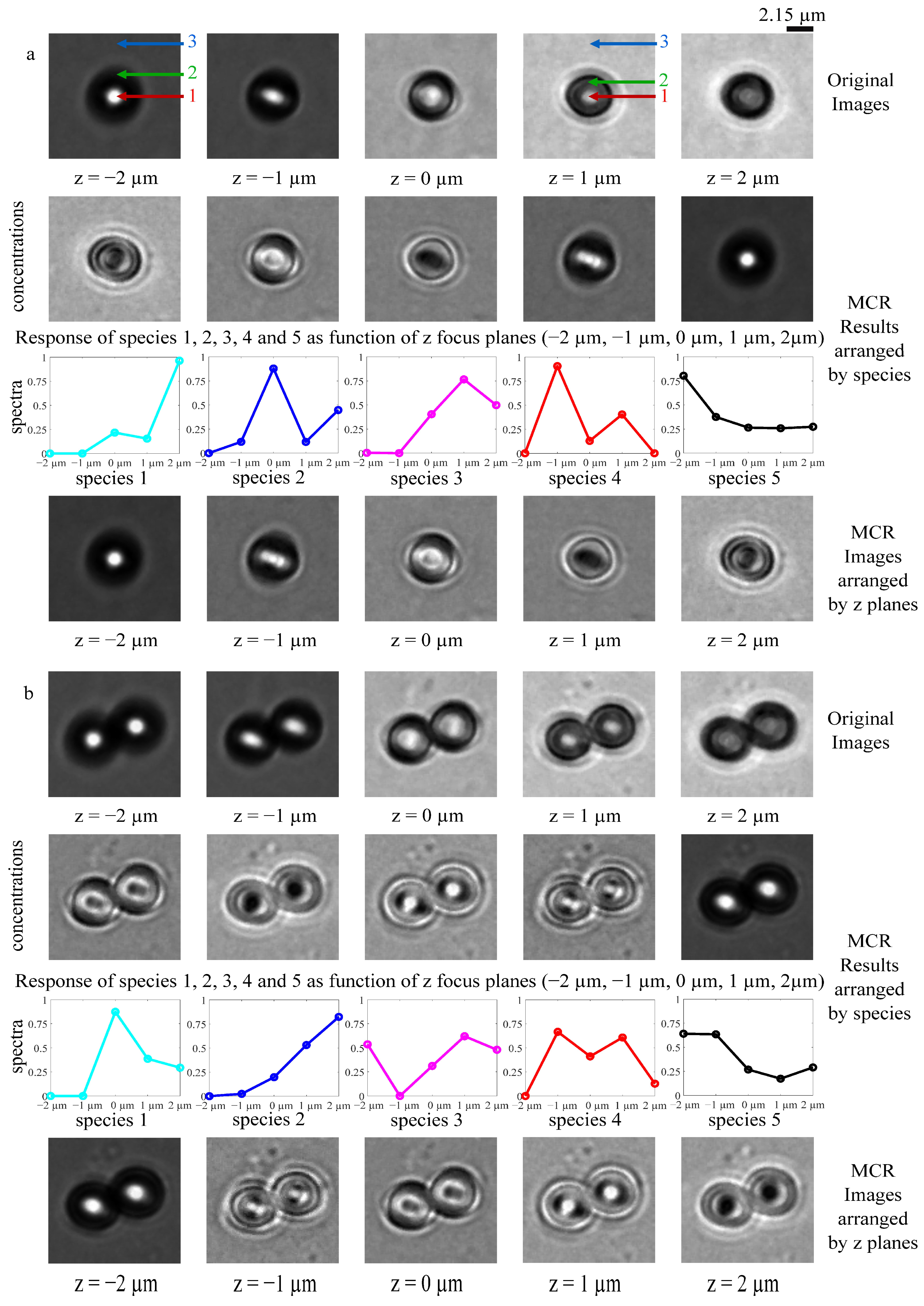
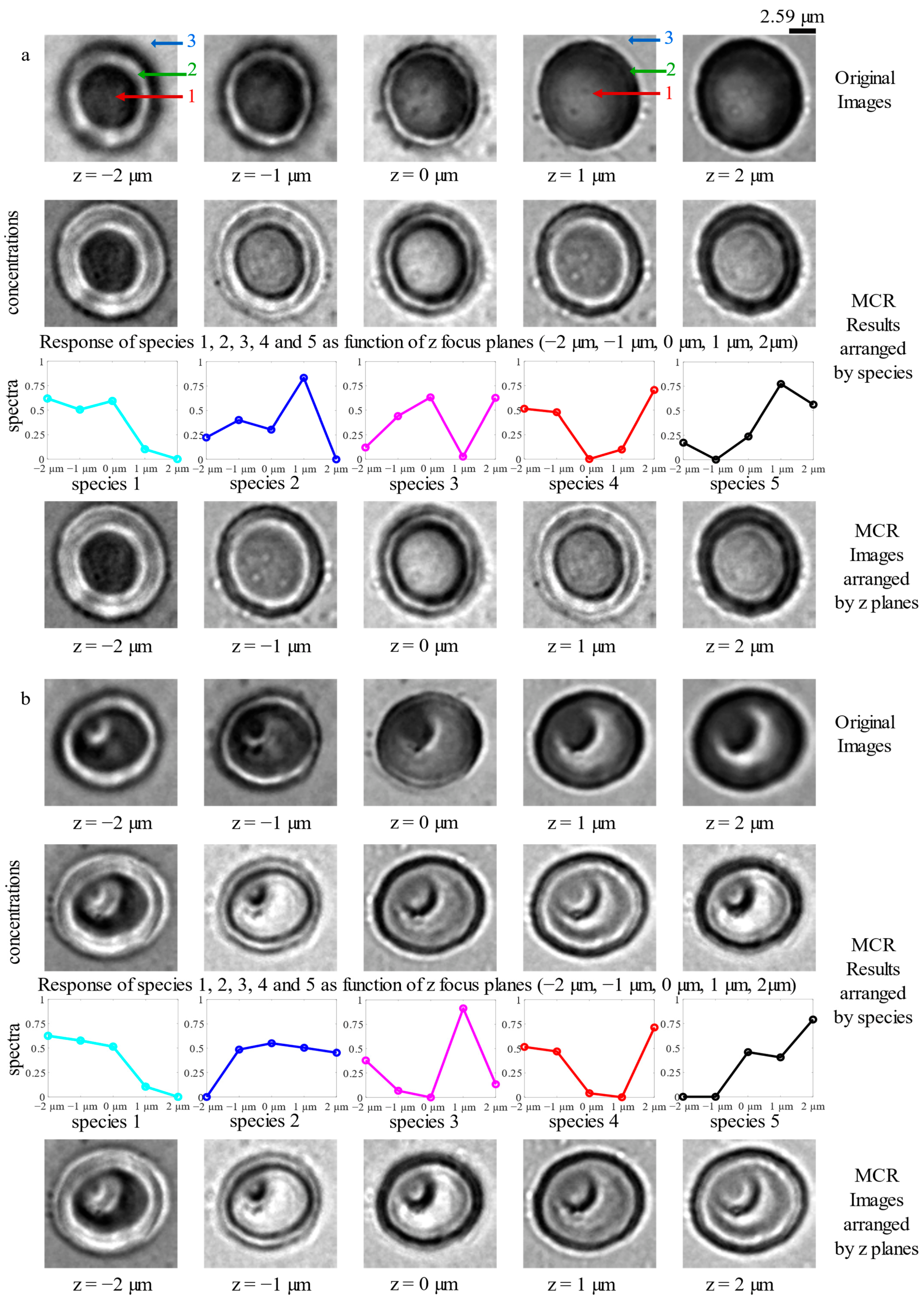
4.1. Multiplane Image Restoration of 3D Objects

The images and spectra obtained from the MCR analysis are presented first. In Figure 2 contains images of a single (a) and two (b) silica microbeads, and in Figure 3, there are images of an assumed-to-be-healthy erythrocyte (a) and an erythrocyte with a suspected parasite or parasite by-product within the cell (b). For each sample, both the pre-processed images acquired using the brightfield microscope and those resulting from the MCR analysis under non-negativity constraints are presented and compared. The original pre-processed images are arranged plane by plane, while the images obtained from the MCR analysis are arranged by species. The images from the MCR analysis are then ordered plane by plane. Each image is displayed between the maximum and minimum values of its own pixels. One of the findings is that the MCR analysis reduces the initial blur which therefore leads to sharper images with more pronounced edges.
Four regions can be distinguished on the original images. The first three regions are given by the numbers 1, 2, and 3 in the silica microbead and RBC original images at z = 2   µ m and at z = 1   µ m , repsectively. Regions 1 and 2 are the central parts of the samples that can be defined by the light extinction process that is specific to the sample’s optical properties. This central part is of great interest because it can provide the details regarding the volume content. Region 3 is the background-focused image, which is composed mainly of dried distilled water for the silica microbead and plasma for the erythrocyte. Region 4 is the region between the second one and the third one. It shows the sample edge, with the pixels intensity fluctuations due to the sample thickness, in addition to the refraction of light resulting from the changes in the refractive indices from the air to the sample. For the microbead, region 1 corresponds to the part of the sample that is closest to the objective. In the laser-source-to-CMOS-camera direction, this region is bright for the planes in front of the objective lens focal plane, and it is dark for the planes behind the objective lens focal plane. The same observation can be made with the erythrocyte sample, except that the part closest to the objective is now region 2. This observation, which tends to challenge the natural symmetry idea of the samples, is partly due to the aberrations of the objective lens, and it may have an influence on the reconstructed images. The MCR analysis allows us to recover regions 1 and 2 without any real correction of the differences in the grayscale due to the lens effect. For the assumed-to-be-healthy RBC that has a biconcave shape at rest, for example, the sections in the center are a disc, and those near the ends are rings. The MCR results are closer to this representation compared to the original images (see Figure 4), but region 1 and region 2 do not have same grayscale intensities at z = 2   µ m and z = 2   µ m . For the RBC with a suspected infection, the result is different. The biconcave shape is less well reconstructed for all of the planes, except for the plane at z = 2   µ m ; traces of the internal presence can be nevertheless noticed, and we suspect this internal presence is the origin of this difference. This presence, which was revealed after the MCR analysis for the planes z = 1   µ m , z = 0   µ m , z = 1   µ m , and z = 2   µ m , presents an earphone shape that is specific to the malaria parasite at the trophozoite stage. This earphone shape is not visible on the original images; this suggests that the MCR analysis can reveal the presence of hidden inner components. Moreover, the fact that the expected disc at the center from a biconcave shape was not retrieved for the plane z = −2 µm could mean that the parasite is in a part of the cell that is further from this plane, and in addition, that the cell is not at an advanced infection level. This clearly demonstrates that the MCR analysis is capable of providing information about the characterization of a target volume, especially for a biological sample. Our results suggest that brightfield microscopy coupled with MCR analysis can be an alternative, simple, and cost-effective 3D microscopy imaging technique.

4.2. Comparison with 3D Deconvolution

In order to compare this technique to the well-known 3D deconvolution methods, images from 3D deconvolution methods, such as Wiener filtering, Richardson–Lucy, and blind deconvolution, are presented in Figure 5 and Figure 6. For the microbead silica images, the MCR images are the sharpest ones, except for the images at z = 0   µ m . For RBC, the MCR images are sharpest ones for all of the planes, and the reconstructed images are more faithful to the expected shape. The images were then statistically compared using a set of No Reference Images Quality Metrics (NR-IQMs), which are: Standard Deviation (SD), ENTROPY, Average Gradient (AG), and Auto Correlation (AC). Figures S1–S4 in the Supplementary Materials give, respectively, the NR-IQMs values for a single silica microbead, a pair of microbeads, the assumed-to-be-healthy RBC, and the RBC with a suspected infection. The SD values of the MCR images are the lowest ones. This indicates that the MCR images have more contrast, as can be observed. The MCR images present the best values of ENTROPY only for the RBC images. This is more noticeable for the RBC with the inner earphone shape, which represents the set of samples with the most information about its volume. This suggests that the technique would work better for samples with less obvious volume structures. A study on the different types of volumetric shape would allow one to learn the limits of this assertion. As in the case of SD, one would expect that the values of AG would be better in the case of MCR. However, AG, in addition to being a measure of contrast, is a measure of clarity; this may explain why the highest values are those of Richardson–Lucy, which present with the blind deconvolution, the brightest images. It can even be seen that the values of AG for the blind deconvolution images are just as high and are close to those of Richardson–Lucy. The best AC values were obtained for the MCR images. This indicates that MCR images have edges that are less smooth and are less blurred compared to those of the deconvolution images. The improvements observed with MCR are mainly due to the fact that the methodology described here retrieves ballistic photons, which are known as the photons that come from the in-focus section. A reconstruction based on such a recovery eliminates the noise more efficiently. This will be more justified with objects that have absorbing properties, whose contrast and feature objects are more enhanced. In these cases, MCR offers an advantage over the classical deconvolution methods, which present an overlap issue which is increased here by the use of an emission PSF applied to the inverted grayscale images of the absorption samples. Ballistics photons, as well as in-focus and some out-of-focus scattering photons, are recovered, hence, there is blurring. Therefore, the MCR analysis can be an alternative to the 3D deconvolution methods in 3D brightfield microscopy.

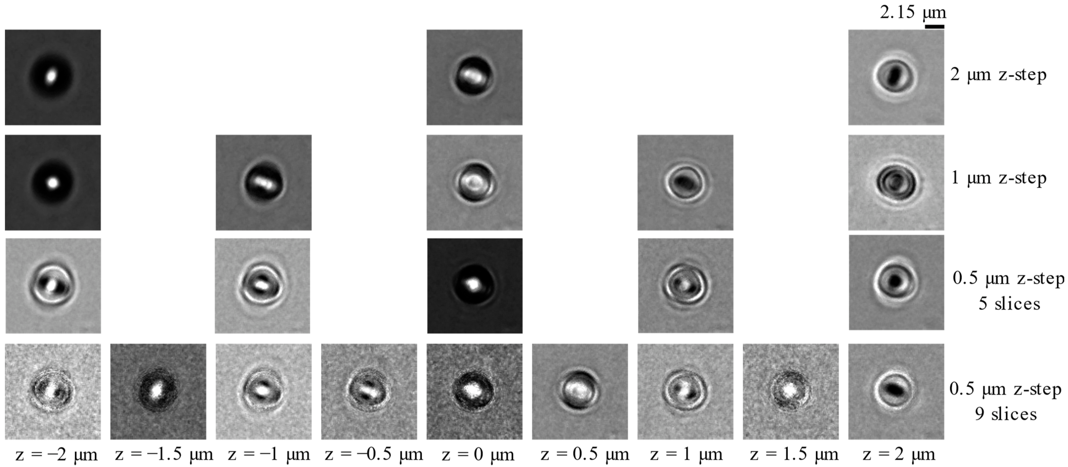
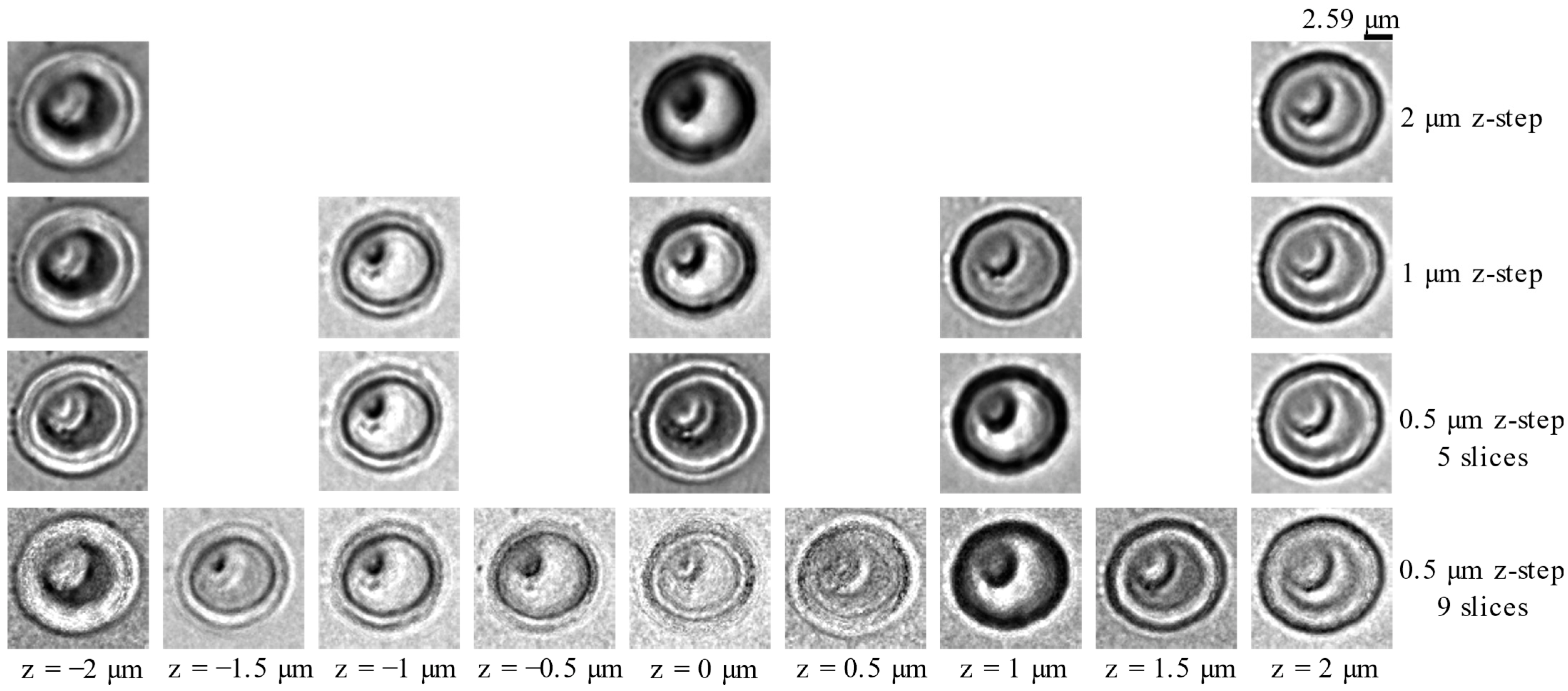
4.3. Influence of the z-Step Value

This part of the study aims to evaluate the resulting z-resolution of the method from the algorithm performance point of view. The study was conducted in two stages to obtain a judgment about which step achieves the results which are most satisfying. The first one evaluates the influence of the z-step on the reconstruction performance regarding the number of images recovered. The second one shows that the method is not image number dependent.
The influence of the z-step on the reconstruction performance is evaluated by conducting three z-steps, which are: 2 µm, 1 µm, and 0.5 µm. The analysis is made on a 4 µm focal length, thus, three images for the 2 µm z-step, five images for 1 µm z-step, and nine images for 0.5 µm z-step were recorded. For the 0.5 µm z-step, two results are presented, and there is one where nine planes were recovered from the nine images recorded, and there is another one where five planes were recovered. Indeed, the retrieval of five planes from nine images allowed us to double the number of samples along the z-axis. The MCR algorithm was applied to the images of single silica microbeads and RBC with an inner earphone shape. The MCR images for these different z-steps are given in Figure 7, for the single microbead, and in Figure 8, for the RBC with inner earphone shape. The images with 2 µm z-step are blurred compared to the one that was acquired in the 1µm z-step, and it can be even observed that for RBC with the inner earphone-shape images, the edges are more spread out on the planes z = 0 µm and z = 2 µm. Additionally, there are recovered planes in the 0.5 µm and 1 µm z-step reconstructions, which are not present in the 2 µm z-step reconstruction, for example, the images on the z = −1 µm plane for the microbead and the RBC. This suggest that the use of 2 µm z-step cause a lack of information on the 3D structure of the sample. This could be due to under sampling. The images of nine planes recovered in the 0.5 µm z-step are noisy and do not provide new sections compared to the 1 µm z-step images. The images of five planes recovered in the 0.5 µm step compared to the ones recovered for 1 µm z-step are similar for the RBC, but they have more pronounced contours. For the silica microbead, the five planes recovered in the 0.5 µm step are brighter than the ones recovered in the 1 µm z-step, and they present notable differences. Three NR-IQMs, which are SD, ENTROPY, and AC, have been calculated, and they are presented in Figure S5 in the Supplementary Materials. The values are similar for both of them. Thus, the sampling according to the Nyquist criterion does not seem to provide additional information on the 3D structure of the sample. This result is obtained because sampling according to the Nyquist criterion was not applied to the axial resolution, but it was applied to the depth of field. In line with Abbe’s criterion, our microscope has an axial resolution of 2 µm. The Nyquist criterion corresponds, in this case, to the depth of field.
In the following, an analysis was performed on the 0.5 µm z-step recorded images to rule out the possibility that the method would be depend on the number of reconstructed planes. Three new sets of images were obtained as follows: the images from z = −2 µm to z = 0 µm make up the left sample, the images from z = −1 µm to z = 1 µm make up the middle sample, and the images from z = 0 µm to z = −2 µm make up the right sample. The images obtained (see Figures S6 and S7 in the Supplementary Materials) were still very noisy, which confirmed the idea that the quality of the image reconstructed by the MCR analysis is not related to numbers of the image, but it is probably related to the sampling z-step. The depth of field therefore fixes the suitable z-scanning step in the MCR analysis. It is important to keep in mind that we cannot make a direct interpretation of the similarity or dissimilarity of the slices in Figures S6 and S7, since the data supplied to the MCR algorithm for the left sample, the middle sample, and the right sample are not the same.

5. Conclusions

The MCR analysis of the z-scanning images achieved 3D information recovery in conventional brightfield microscopy. The developed method is an alternative, simple, and cost-effective 3D microscopy technique. In this study, we demonstrated a bilinear relationship between the z-scanning images of brightfield microscopy in the transmission mode and both the specimen layers’ concentrations and spectra. The transmittance mixture images are thus described as MCR data sets. The MCR-ALS analysis under a non-negativity constraint that is commonly used for hyperspectral imaging was applied to four data sets of silica microbeads and RBCs. The images obtained from the MCR analysis demonstrate the proposed method’s ability to perform 3D information recovery through multiplane images deblurring, contrast improvement, and object features enhancement, especially for biological specimen. In comparison with the 3D deconvolution methods, MCR analysis produces better results, showing that it can be an alternative to 3D deconvolution methods. A final analysis of the influence of the z-step value showed that the appropriated step for the MCR analysis is the depth of field of the brightfield microscope that is used. This work therefore opens the door to a new 3D brightfield microscopy technique.
Rotational ambiguity remains a major problem for the MCR method, which has not been solved entirely by the non-negativity constraint used here. A study on the application of alternative constraints to the MCR-ALS algorithm would allow us to learn about the constraints, which would improve the results obtained in this work. Additionally, more complex experimental samples would allow us to evaluate the effectiveness of the algorithms of the methodology. Finally, according to Equation (7), the recorded image is related to the concentrations and spectra. The concentration is the number of particles per unit volume. The spectrum is a quantity related to the extinction cross-section, soan occurrence of the extinction process. Thus, a concentration image presents the attenuation of the light by the particles over the volume of the in-focus section. Thus, the methodology developed here could allow us to perform optical sectioning. This could be validated by a comparison with well-known optical sectioning methodologies.

Supplementary Materials

The following supporting information can be downloaded at: https://www.mdpi.com/article/10.3390/photonics10020163/s1, Figure S1: NR-IQMs values of planes recovered for single microbead; Figure S2: NR-IQMs values of planes recovered for the pair of microbeads; Figure S3: NR-IQMs values of planes recovered for the assumed healthy RBC; Figure S4: NR-IQMs values of planes recovered for the RBC with suspected infection; Figure S5: NR-IQMs values of single microbead and RBC with suspected infection for the 1 µm z-step and 0.5 µm z-step images; Figure S6: MCR images of single microbead for left samples (a), middle samples (b), right sample (c), and 0.5 µm z-step (d); Figure S7: MCR images of RBC with inner earphone-shape for left samples (a), middle samples (b), right sample (c), and 0.5 µm z-step (d).

Author Contributions

Conceptualization, J.T.Z.; methodology, S.B.D.; software, S.B.D., D.J.F.U.A., A.M.A. and J.T.Z.; validation, S.B.D., D.J.F.U.A., A.M.A. and J.T.Z.; formal analysis, S.B.D., D.J.F.U.A. and A.M.A.; investigation, S.B.D., D.J.F.U.A. and A.M.A.; resources, S.B.D., A.M.A. and J.T.Z.; data curation, S.B.D.; writing—original draft preparation, S.B.D. and A.M.A.; writing—review and editing, S.B.D., D.J.F.U.A., A.M.A. and J.T.Z.; visualization, S.B.D. and A.M.A.; supervision, J.T.Z.; project administration, J.T.Z.; funding acquisition, J.T.Z. All authors have read and agreed to the published version of the manuscript.

Funding

This work was supported by SIDA (the Swedish International Development Cooperation Agency) through ISP (the International Science Programme, Uppsala University).

Institutional Review Board Statement

Not applicable.

Informed Consent Statement

Not applicable.

Data Availability Statement

The datasets used and/or analysis results obtained in the current study are available from the corresponding author on request.

Acknowledgments

The authors thank Silué from the laboratory of the Regional Hospital Center for the biological sample preparation.

Conflicts of Interest

The authors declare no conflict of interest.

References

  1. Helmchen, F.; Denk, W. Deep tissue two-photon microscopy. Nat. Methods 2005, 2, 932–940. [Google Scholar] [CrossRef] [PubMed]
  2. Conchello, J.A.; Lichtman, J.W. Optical sectioning microscopy. Nat. Methods 2005, 2, 920–931. [Google Scholar] [CrossRef] [PubMed]
  3. Sarder, P.; Nehorai, A. Deconvolution methods for 3-D fluorescence microscopy images. IEEE Signal Process. Mag. 2006, 23, 32–45. [Google Scholar] [CrossRef]
  4. Biggs, D.S.C. 3D Deconvolution Microscopy. Curr. Protoc. Cytom. 2010, 52, 12.19.1–12.19.20. [Google Scholar] [CrossRef]
  5. Dan, D.; Yao, B.; Lei, M. Structured illumination microscopy for super-resolution and optical sectioning. Chin. Sci. Bull. 2014, 59, 1291–1307. [Google Scholar] [CrossRef]
  6. Paddock, S.W. Principles and practices of laser scanning confocal microscopy. Mol. Biotechnol. 2000, 16, 127–149. [Google Scholar] [CrossRef]
  7. Patel, D.V.; McGhee, C.N. Quantitative analysis of in vivo confocal microscopy images: A review. Surv. Ophthalmol. 2013, 58, 466–475. [Google Scholar] [CrossRef]
  8. König, K. Multiphoton microscopy in life sciences. J. Microsc. 2001, 200, 83–104. [Google Scholar] [CrossRef]
  9. Langhorst, M.F.; Schaffer, J.; Goetze, B. Structure brings clarity: Structured illumination microscopy in cell biology. Biotechnol. J. 2009, 4, 858–865. [Google Scholar] [CrossRef]
  10. Jost, A.; Heintzmann, R. Superresolution Multidimensional Imaging with Structured Illumination Microscopy. Annu. Rev. Mater. Res. 2013, 43, 261–282. [Google Scholar] [CrossRef]
  11. Saxena, M.; Eluru, G.; Gorthi, S.S. Structured illumination microscopy. Adv. Opt. Photonics 2015, 7, 241–275. [Google Scholar] [CrossRef]
  12. Sanderson, J. Light Sheet Microscopy. In Understanding Light Microscopy, 1st ed.; Sanderson, J., Ed.; Wiley: Hoboken, NJ, USA, 2019; pp. 483–506. [Google Scholar] [CrossRef]
  13. Wan, Y.; McDole, K.; Keller, P.J. Light-Sheet Microscopy and Its Potential for Understanding Developmental Processes. Annu. Rev. Cell Dev. Biol. 2019, 35, 655–681. [Google Scholar] [CrossRef]
  14. Tadrous, P.J. A method of PSF generation for 3D brightfield deconvolution. J. Microsc. 2010, 237, 192–199. [Google Scholar] [CrossRef]
  15. Yao, S.; Mills, J.K.; Ajamieh, I.A.; Li, H.; Zhan, X. Automatic three-dimensional imaging for blastomere identification in early-stage embryos based on brightfield microscopy. Opt. Lasers Eng. 2020, 130, 106093. [Google Scholar] [CrossRef]
  16. McNally, J.G.; Karpova, T.; Cooper, J.; Conchello, J.A. Three-Dimensional Imaging by Deconvolution Microscopy. Methods 1999, 19, 373–385. [Google Scholar] [CrossRef]
  17. Icha, J.; Weber, M.; Waters, J.C.; Norden, C. Phototoxicity in live fluorescence microscopy, and how to avoid it. Bioessays 2017, 39, 1700003. [Google Scholar] [CrossRef]
  18. Lac, A.; Le Lam, A.; Heit, B. Optimizing Long-Term Live Cell Imaging. In Fluorescent Microscopy; Heit, B., Ed.; Humana: New York, NY, USA, 2022; Volume 2440, pp. 57–73. [Google Scholar] [CrossRef]
  19. Streibl, N. Three-dimensional imaging by a microscope. J. Opt. Soc. Am. A 1985, 2, 121–127. [Google Scholar] [CrossRef]
  20. Maa, X.; Zhanga, Z.; Yaoa, M.; Penga, J.; Zhonga, J. Spatially-incoherent annular illumination microscopy for bright-field optical sectioning. Ultramicroscopy 2018, 195, 74–84. [Google Scholar] [CrossRef]
  21. Candia, C.N.H.; Gutiérrez-Medina, B. Direct Imaging of Phase Objects Enables Conventional Deconvolution in Bright Field Light Microscopy. PLoS ONE 2014, 9, e89106. [Google Scholar] [CrossRef]
  22. Holmes, T.J.; O’Connor, N.J. Blind deconvolution of 3D transmitted light brightfield micrographs. J. Microsc. 2000, 200, 114–127. [Google Scholar] [CrossRef]
  23. Agnero, M.A.; Konan, K.; Tokou, Z.G.C.S.; Kossonou, Y.T.A.; Dion, B.S.; Kaduki, K.A.; Zoueu, J.T. Malaria-Infected Red Blood Cell Analysis through Optical and Biochemical Parameters Using the Transport of Intensity Equation and the Microscope’s Optical Properties. Sensors 2019, 19, 3045. [Google Scholar] [CrossRef]
  24. Aguet, F.; Van de Ville, D.; Unser, M. Model-based 2.5-D deconvolution for extended depth of field in brightfield microscopy. IEEE Trans. Image Process. 2008, 17, 1144–1153. [Google Scholar] [CrossRef] [PubMed]
  25. Praveen, P.A.; Arockiaraj, F.G.; Gopinath, S.; Smith, D.; Kahro, T.; Valdma, S.-M.; Bleahu, A.; Ng, S.H.; Reddy, A.N.K.; Katkus, T.; et al. Deep Deconvolution of Object Information Modulated by a Refractive Lens Using Lucy-Richardson-Rosen Algorithm. Photonics 2022, 9, 625. [Google Scholar] [CrossRef]
  26. Gutiérrez-Medina, B. Optical sectioning of unlabeled samples using brightfield microscopy. Proc. Natl. Acad. Sci. USA 2022, 119, e2122937119. [Google Scholar] [CrossRef] [PubMed]
  27. Solomon, C.; Breckon, T. Image restoration. In Fundamentals of Digital Image Processing: A Practical Approach with Examples in Matlab; Solomon, C., Breckon, T., Eds.; Wiley-Blackwell: Hoboken, NJ, USA; Oxford, UK, 2011; pp. 141–167. [Google Scholar] [CrossRef]
  28. Gonzalez, R.C.; Woods, R.E. Image restoration. In Digital Image Processing, 2nd ed.; Gonzalez, R.C., Woods, R.E., Eds.; Prentice Hall: Hoboken, NJ, USA, 2002; pp. 220–281. [Google Scholar]
  29. Holmes, T.J.; Bhattacharyya, S.; Cooper, J.A.; Hanzel, D.; Krishnamurthi, V.; Lin, W.; Roysam, B.; Szarowski, D.H.; Turner, J.N. Light Microscopic Images Reconstructed by Maximum likelihood Deconvolution. In Handbook of Biological Confocal Microscopy; Pawley, J.B., Ed.; Springer: Boston, MA, USA, 1995; pp. 389–402. [Google Scholar] [CrossRef]
  30. Law, N.F.; Lane, R.G. Blind deconvolution using least squares minimisation. Opt. Commun. 1996, 128, 341–352. [Google Scholar] [CrossRef]
  31. Biggs, D.S.C.; Andrews, M. Acceleration of iterative image restoration algorithms. Appl. Opt. 1997, 36, 1766–1775. [Google Scholar] [CrossRef] [Green Version]
  32. Aguet, F.; Van De Ville, D.; Unser, M. An accurate PSF model with few parameters for axially shift-variant deconvolution. In Proceedings of the 2008 5th IEEE International Symposium on Biomedical Imaging: From Nano to Macro, Paris, France, 14–17 May 2008; pp. 157–160. [Google Scholar] [CrossRef]
  33. Gibson, S.F.; Lanni, F. Experimental test of an analytical model of aberration in an oil-immersion objective lens used in three-dimensional light microscopy. J. Opt. Soc. Am. A 1991, 8, 1601–1613. [Google Scholar] [CrossRef]
  34. Offroy, M. Développement de la Super-Résolution Appliquée à L'imagerie des Spectroscopies Vibrationnelles. Ph.D. Thesis, Université de Lille 1, Lille, France, 17 January 2012. Available online: https://tel.archives-ouvertes.fr/tel-00687944 (accessed on 9 January 2023).
  35. de Juan, A.; Jaumot, J.; Tauler, R. Multivariate Curve Resolution (MCR). Solving the mixture analysis problem. Anal. Methods 2014, 6, 4964–4976. [Google Scholar] [CrossRef]
  36. Rutan, S.C.; de Juan, A.; Tauler, R. Introduction to Multivariate Curve Resolution. In Comprehensive Chemometrics; Brown, S.D., Tauler, R., Walczak, R., Eds.; Elsevier: Oxford, UK, 2009; pp. 249–259. [Google Scholar]
  37. de Juan, A.; Tauler, R. Multivariate Curve Resolution (MCR) from 2000: Progress in Concepts and Applications. Crit. Rev. Anal. Chem. 2007, 36, 163–176. [Google Scholar] [CrossRef]
  38. Hamilton, J.C.; Gemperline, P.J. Mixture analysis using factor analysis. II: Self-modeling curve resolution. J. Chemom. 1990, 4, 1–13. [Google Scholar] [CrossRef]
  39. de Juan, A.; Tauler, R. Chemometrics applied to unravel multicomponent processes and mixtures: Revisiting latest trends in multivariate resolution. Anal. Chim. Acta 2003, 500, 195–210. [Google Scholar] [CrossRef]
  40. Duponchel, L.; Elmi-Rayaleh, W.; Ruckebusch, C.; Huvenne, J.P. Multivariate Curve Resolution Methods in Imaging Spectroscopy: Influence of Extraction Methods and Instrumental Perturbations. J. Chem. Inf. Comput. Sci. 2003, 43, 2057–2067. [Google Scholar] [CrossRef]
  41. Windig, W.; Guilment, J. Interactive self-modeling mixture analysis. Anal. Chem. 1991, 63, 1425–1432. [Google Scholar] [CrossRef]
  42. Van Benthem, M.H.; Keenan, M.R. Fast algorithm for the solution of large-scale non-negativity-constrained least squares problems. J. Chemom. 2004, 18, 441–450. [Google Scholar] [CrossRef]
  43. Van Benthem, M.H.; Keenan, M.R.; Haaland, D.M. Applications on equality constraints on variables during alterning least squares procedures. J. Chemom. 2002, 16, 613–622. [Google Scholar] [CrossRef]
  44. Golshana, A.; Abdollahia, H.; Maederb, M. The reduction of rotational ambiguity in soft-modeling by introducing hard models. Anal. Chim. Acta 2012, 709, 32–40. [Google Scholar] [CrossRef]
  45. Hugeliera, S.; Devosa, O.; Ruckebuscha, C. On the implementation of spatial constraints in multivariate curve resolution alternating least squares for hyperspectral image analysis. J. Chemom. 2015, 29, 557–561. [Google Scholar] [CrossRef]
  46. Hugelier, S.; Piqueras, S.; Bedia, C.; de Juan, A.; Ruckebusch, C. Application of a sparseness constraint in multivariate curve resolution—Alternating least squares. Anal. Chim. Acta 2018, 1000, 100–108. [Google Scholar] [CrossRef]
  47. de Juan, A.; Maeder, M.; Hancewicz, T.; Tauler, R. Use of local rank-based spatial information for resolution of spectroscopic images. J. Chemom. 2008, 22, 291–298. [Google Scholar] [CrossRef]
  48. Omucheni, D.L.; Kaduki, K.A.; Bulimo, W.D.; Angeyo, H.K. Application of principal component analysis to multispectral-multimodal optical image analysis for malaria diagnostics. Malar. J. 2014, 13, 485. [Google Scholar] [CrossRef]
  49. Mishchenko, M.I.; Hovenier, J.W.; Mackowski, D.W. Single scattering by a small volume element. J. Opt. Soc. Am. A 2004, 21, 71–87. [Google Scholar] [CrossRef] [PubMed]
  50. Mishchenko, M.I.; Liu, L.; Videen, G. Conditions of applicability of the single scattering approximation. Opt. Express 2007, 15, 7522–7527. [Google Scholar] [CrossRef] [PubMed]
  51. Ma, L.; Zhai, J.; Wang, C. Investigation of the single scattering approximation through direct electromagnetic scattering simulation. OSA Contin. 2021, 4, 2496–2509. [Google Scholar] [CrossRef]
  52. Wang, L.V.; Wu, H.I. Ballistic Imaging and Microscopy. In Biomedical Optics: Principles and Imaging; Wang, L.V., Wu, H.I., Eds.; John Wiley & Sons: Hoboken, NJ, USA, 2007; pp. 153–179. [Google Scholar] [CrossRef]
Figure 1. Brightfield optical microscope in transmission mode.
Photonics 10 00163 g001
Figure 2. Pre-processed brightfield microscope images and results from MCR analysis for a single silica microbead (a) and a pair of silica microbeads (b).
Photonics 10 00163 g002
Figure 3. Pre-processed brightfield microscope images and results from MCR analysis for assumed-to-be-healthy erythrocyte (a) and an erythrocyte with a suspected infection (b).
Photonics 10 00163 g003
Figure 4. Images of simulated biconcave sections: original and MCR images.
Photonics 10 00163 g004
Figure 5. Original, Wiener filtering, Richardson–Lucy, blind deconvolution, and MCR images of a single silica microbead (a) and a pair of silica microbeads (b).
Photonics 10 00163 g005
Figure 6. Original, Wiener filtering, Richardson–Lucy, blind deconvolution, and MCR images of assumed-to-be-healthy RBC (a) and RBC with a suspected infection (b).
Photonics 10 00163 g006
Figure 7. MCR images of single microbead for different z-steps.
Photonics 10 00163 g007
Figure 8. MCR images of RBC with inner earphone shape for different z-steps.
Photonics 10 00163 g008
Disclaimer/Publisher’s Note: The statements, opinions and data contained in all publications are solely those of the individual author(s) and contributor(s) and not of MDPI and/or the editor(s). MDPI and/or the editor(s) disclaim responsibility for any injury to people or property resulting from any ideas, methods, instructions or products referred to in the content.

