Article

All-Fiber Pulse-Train Optical Frequency-Domain Interferometer for Dynamic Absolute Distance Measurements of Vibration

1
National Key Laboratory of Shock Wave and Detonation Physics, Institute of Fluid Physics, China Academy of Engineering Physics, Mianyang 621900, China
2
China Academy of Engineering Physics, Mianyang 621900, China
*
Author to whom correspondence should be addressed.
Photonics 2023, 10(12), 1342; https://doi.org/10.3390/photonics10121342
Submission received: 2 November 2023 / Revised: 2 December 2023 / Accepted: 4 December 2023 / Published: 5 December 2023
(This article belongs to the Special Issue Advanced Photonics Sensors, Sources, Systems and Applications)

Abstract

:
In this paper, we propose an all-fiber co-axial optical frequency-domain interferometer (OFDI) in a pulse-train mode with a sample rate of 9 kHz for measuring the vibrations in an internal structure without any contact. It was subjected to a range of 4.555 mm and had an accuracy level of 0.006 mm, as confirmed by a linear motion experiment. Due to the precise time synchronization for reducing the background light leakage and suppressing the dynamic fuzziness, the proposed OFDI could realize the dynamic absolute distance measurements of the vibration process under harmonic excitation with frequencies ranging from 200 Hz to 1800 Hz. The characteristic parameters of vibration could be analyzed using the acquired distance results. Furthermore, the OFDI system obtained the frequency conversion as the time under anharmonic periodic excitation with a sweeping rate of 3600 Hz/s. The measurement performance for the vibration velocity compared with the displacement interferometer system for any reflector (DISAR) was demonstrated in a harmonic excitation experiment. The proposed method expands the application of all-fiber OFDI technology from static to dynamic scenes.

1. Introduction

Vibration measurement technology for internal structure modal tests and analyses plays an essential role in scientific research and industrial manufacturing, such as in the automotive and aerospace industries [1,2]. Recently, there has been a dramatic interest in developing vibration measurement sensors and devices with excellent performance capabilities [3,4]. Of these, the accelerometer is the most used and mature sensor in vibration and pressure measurement, owing to its high reliability and broadband responsibility. However, the performance of the accelerometer under high-frequency excitation is adversely affected by the mass loading effect of the contacting method.
Non-contact vibration measurement technologies, based on optical interferometry, have recently attracted considerable interest and shown significant application potential. There are two major types of optical vibration measurement technologies. One is the video camera type, which is represented by electronic speckle pattern interferometry (ESPI) [5], digital speckle shearography (DSS) [6], digital image correlation (DIC) [7], and digital holographic interferometry (DHI) [8]. Due to the implementation of high-speed CCD or CMOS cameras, they can acquire a full-field vision of the measured object in real time with great precision and high spatial resolution. However, when these mentioned technologies are employed in the vibration measurement of internal structures, the drawbacks emerge gradually, especially in practical engineering applications. The cumbersome video camera is impossible to install on a centrifuge or compound vibration platform. Therefore, a particular light path should be designed to guide the beam through the structures’ gaps to the measured object. As a result, this will change the intrinsic status of internal structures.
The other vibration measurement technology is an optical interferometric type, represented by time-of-flight (TOF) detection, low-coherence interferometry (LCI), and homodyne or heterodyne laser Doppler vibrometers (LDV). The TOF detection method [9], based on an electro-optic-sampling-based timing detector, can measure the relative temporal positions of optical pulses using all-fiber differential-biased Sagnac loop interferometers. This technology demonstrates fast displacement in real time, with tens of nanometers of precision for the acquisition of several nanoseconds. Although the measurement range is up to 6 mm as the rising edge of the photocurrent pulse is ~40 ps long, the cost of the system increases dramatically due to the use of high-bandwidth photodiodes and oscilloscopes. The LCI technique has generated considerable interest in industrial applications resulting from its precise measurement of the location of a zero optical path difference. The typical types of LCI, such as Fourier domain LCI [10] and polarized LCI [11], display high speeds of up to tens of kHz with an optical detector or camera and can process the resolution and accuracy of several nanometers. However, the measuring range of LCI is achieved in millimeters due to the short coherence length of the light source. Recently, a novel Fourier domain LCI based on a spatial heterodyne spectrometer [12] has been shown to reach measurable optical depths of nearly 5 cm with a theoretically calculated resolution of 5 μm. However, the optical path in the spectrometer is complex, and it continues to be constructed with bulky elements and a CMOS camera. The disadvantages of the cumbersome structure are shared by video camera-type vibration measurement systems. Moreover, the maximum range depends on the camera detector size of the heterodyne spectrometer.
In an LDV system [13,14], the frequency shifting of the signal beam, directly proportional to the object’s velocity, is detected by interferometry with the reference beam. The use of a photodiode can expand the response bandwidth to megahertz. Moreover, the ellipse-fitting compensated method (Heydemann correction) [15] for phase difference signals can realize a displacement resolution on the nanometer scale. The development of all-fiber LDV [16,17] has reduced the difficulty of beam guidance inside complicated structures. The interferometry signal beam can be transmitted to a measured object through the flexible implementation of fiber. In order to create a pair of in-phase and quadrature signals to reconstruct the actual phase change as a vibration, the propagation of the reference beam should be off-axial from the signal beam. In practical engineering experiments, the signal beam travels far (meters or kilometers) from the test room to the vibration platform in fiber. Complex environmental effects, such as high temperatures and strong shocks, readily produce unsteady beam intensity fluctuance, which creates additional cyclic errors in the phase of the interferometric signal, even if the response parameter’s calibration has been executed before the experiments. The additional cyclic errors make the ellipse-fitting of the Lissajous curve valid in several vibration periods, corresponding to a millisecond in the vibration frequency of kilohertz. Significantly, the fundamental measurement principle of the mentioned technologies is the partial coherence between the interferometric beams in the time or space domains. Therefore, only displacement proportional to the optical path difference can be acquired during the testing period. The absolute positional relationship between components in a structure cannot be monitored through the experiment process flow, such as assembling, testing, and transporting.
In 1976, L. Mandel presented a definition of spectral coherence complex degrees and cross-spectral purity [18], and it illustrated the production of the interference fringes observed in the frequency domain, i.e., the energy distribution as a function of the frequency obtained by the superposition of partially and spatially coherent beams with different light paths. According to the spectral coherence theory, an optical frequency-domain interferometer (OFDI) can realize the absolute distance or relative motion measurement in an ultra-fast dynamic process, such as shockwave propagation induced by ultra-intense short-pulse laser pump-probe technology [19]. In recent years, all-fiber OFDI has been developed [20], which is more compact, flexible, and robust than distance measurement technology based on bulky optical elements such as LCI. The structures of co-axial light paths have long-distance ranges of more than 100 mm, which transcend those of TOF and LCI, and high accuracy levels of above 5 μm. However, limited by the scanning mode of spectrum recording under continuous light source operations, the developed system can only obtain a sample rate of up to several hertz, and so it cannot be used in dynamic motion tests such as rotation and vibration with high frequencies. Therefore, this traditional all-fiber OFDI technology is only employed in static distance measurements.
In this work, we present an all-fiber co-axial OFDI working in a pulse-train mode and demonstrate its use in vibration experiments. Firstly, we propose a pulse-train OFDI configuration with a sample rate of a kHz level based on a high-speed line-array detector. A precise time synchronization method is utilized to reduce the background light leakage to improve the quality of the OFDI signal and, additionally, to control the exposure time of the line-array detector to suppress the dynamic fuzziness, which makes it possible to realize the vibration measurement. Moreover, a linear-motion measurement experiment to assess the range and accuracy of the proposed system is conducted. Then, vibration experiments on an electro-vibration exciter are implemented to verify the dynamic measurement performance. Dynamic absolute distance measurement results under two typical excitation modes, harmonic excitation and anharmonic periodic excitation, are displayed and analyzed using the vibration motion equation. The measurement performance of vibration velocity compared with the displacement interferometer system for any reflector (DISAR) is demonstrated in the harmonic excitation experiment. Significantly, the proposed method has excellent practical engineering application potential because the micron-level ranging accuracy is achievable in dynamic vibration measurements.

2. Experimental Method

2.1. The Setup of the Pulse-Train OFDI

The proposed pulse-train OFDI implementation is schematically illustrated in Figure 1a. In all experiments, an electro-vibration exciter (EVE; see Figure 1b), driven by an arbitrary waveform generator (AFG, RIGOL, DG4202), was employed as the vibration source. The target was screw-jointed to the vibration bar of the EVE. A nanosecond pulsed light source (NPLS, FEMIO, FL-3-1550-30-C) ejected a sequence of amplified spontaneous emission (ASE) pulse trains with intervals of 0.111 ms (9 kHz of repetition frequency). For each pulse, the energy was 2 μJ, and the width was 8 ns. A pulse passed through ports 1 to 2 of a three-port fiber circulator (FC) and arrived at a fiber pin (FP, see Figure 1c) mounted on the ferrule clamp isolated to the EVE. The FP was miniaturized with a length of 9 mm and an outside diameter of 2.5 mm. It split the pulse into the following two parts: one part was reflected from the polished front end by the Fresnel principle, which was referred to as the reference pulse, and the other part traveled through the air space between the FP front end and the target, irradiating the target and returning to the FP, and this was referred to as the signal pulse. The two pulses propagated through ports 2 to 3 of the FC and interfered with each other in the frequency domain. As a result, a typical OFDI signal, i.e., a spectrum interference fringe, was produced and recorded in real time by a fiber-optic spectrometer (FOS, OPTOSKY, ATP8730) with a wavelength range of 1527.35 nm–1562.35 nm and an optical resolution of 0.07 nm. The vibration displacement was calculated using the OFDI signal in the off-line mode.
To realize pulse-train OFDI signal-recording, a 1024-pixel line-array detector was embedded in the FOS with a maximum integration time of 0.1 ms. An acoustic optical modulator (AOM, FEMIO, G-1550-80-L-B, Tokyo, Japan) was utilized as a shutter before using the FOS to suppress the dynamic fuzziness induced by the light leakage. Moreover, a pulsed erbium-doped fiber amplifier (P-EDFA, CONNET, FM-1550-1-28e, Shenzhen, China) was arranged after the AOM to compensate for the diffraction loss in the AOM. For the precise time synchronization between the light pulse ejection and optoelectronic component operation, a digital delay generator (DDG, homemade) was triggered by an NPFL, and it sent time-delayed synchronizing signals to the AOM and FOS. As a result, the NPLS, AOM, and FOS operated at the same rate, and the pulse train was transmitted through the AOM and recorded by the FOS chronologically.
Unlike conventional LDV, the proposed OFDI was implemented in a co-axial interferometric structure in which the reference pulse and signal pulse were propagated in nearly identical light paths. The difference between the light paths was only the distance between the FP’s front ends and the targets in air space. When the distance was less than 5 mm, the time interval between the reference pulse and the signal pulse was less than 34 ps, and so these two pulses could overlap in the integrated time of the FOS and produce an OFDI signal. The voltage of one detector pixel can be determined using the following equation:
U m ( f ) = 0 τ G ( f ) I 0 ( f , t ) [ ( a + b ) + 2 a b exp ( 4 π n f D m c + Δ ψ ) ] d t ,
where Um(f) is the translated voltage of the m-th pulse, τ is the integrated time, and G(f) is a gain coefficient as a function of the frequency f, which is mainly related to the combination of the quantum efficiency, area of detector photo surface, and power loss of the system. I0(f,t) is the average light intensity of the individual ejected pulse, a and b are the reflectivity coefficients of the reference pulse and the signal pulse, respectively, which are treated as constants when there is no resonance absorption in the target, Dm is the distance between the FP’s front end and the target when the m-th pulse passes through, n is the refraction index, which is approximately 1 in air space, c is the speed of light in a vacuum, and Δψ is the intrinsic phase difference between the reference pulse and the signal pulse. In an individual pulse, the width is only 8 ns, and the target displacement is no more than 8 nm when the vibration velocity is less than 1 m/s. The tiny displacement could be neglected in the distance calculation, and the Dm in Equation (1) was treated as a constant in the m-th pulse.
The theoretical maximum range of the OFDI could be derived from the optical resolution of the FOS. As demonstrated in Equation (1), the minimum recorded wavelength intervals of the adjacent peaks in the OFDI signal were equal to the optical resolution of the FOS, and so the maximum range could be estimated using the following equation:
D max = λ 0 2 2 n R λ ,
where Dmax is the maximum range, λ0 is the center wavelength of the pulse spectrum, and Rλ is the optical resolution of the FOS.

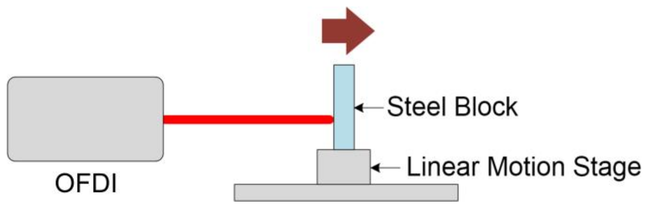
2.2. The Linear Motion Measurement

An experiment on linear motion measurements was conducted to assess the performance, and it included the measurement range and accuracy of the proposed OFDI before the vibration test work. The experimental configuration is shown in Figure 2. A steel block with a roughness of Ra 0.016 was fixed on a linear motion stage. The incremental motion was set to 0.500 mm/step, with an on-axis accuracy of ±0.001 mm. The motion destination was assigned to the point where the OFDI signals were fuzzy and falsely processed.

2.3. The Comparison Measurement with DISAR

We designed a comparison experiment to evaluate the vibration velocity measurement performance of the proposed system, as shown in Figure 3a. Rather than using an FP connected to the OFDI system, we used a microfocus fiber probe (FFP; for details, see Figure 3b) with an outside diameter of 1.1 mm. The reference pulse was still created at the polished front end of single mode (SM) fiber inside the FFP, approximately 4 mm from the optical aperture. A microlens was integrated into the metal holder of the FFP. It could focus the signal pulse on the target to increase the returned light intensity. The light was bent to 90 degrees by a reflector fixed at the end of the holder so that the FFP could be perpendicularly inserted into a narrow gap of less than 15 mm between the EVE body and the target. The distance between the ektexine of FFP and the target was less than 1 mm, which made the vibration measurement system work within the range.
The displacement interferometer system for any reflector (DISAR) [21] was employed for the measurement and compared with the distance differentiation acquired by the proposed method. The center wavelength of DISAR is 1550 nm. The FP used in the vibration measurement in Section 2.1 was connected to DISAR. A photoelectric detector (TianQi, OD-PVX) with a bandwidth of 12 GHz was integrated into the DISAR, and so the measurable maximum velocity was 9.3 km/s. A digital oscilloscope (REGOL, MSO8104) with a bandwidth of 1 GHz and a sample rate of 10 MSa/s was adopted to record the beat frequency produced by the vibrations.

3. Results

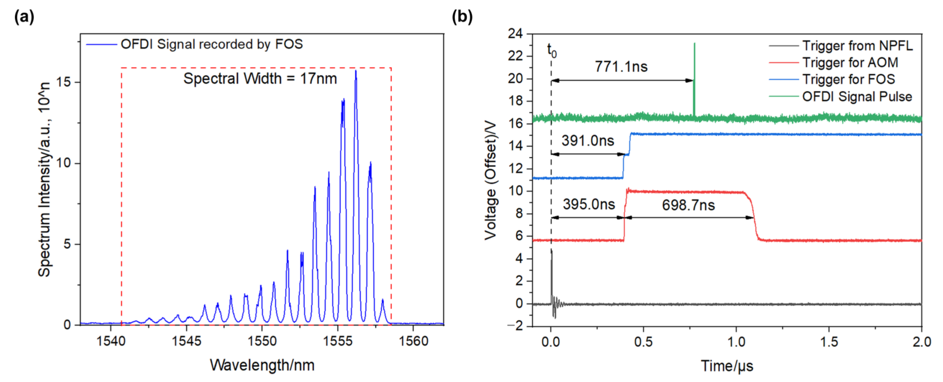
3.1. OFDI Signal and Time Synchronization

A typical OFDI signal recorded by an FOS is shown in Figure 4a. The spectrum spans from 1541 nm to 1558 nm, with a spectral width of 17 nm. Due to the spectral coherence between the reference pulse and the signal pulse, the harmonic power intensity distribution characterized by Equation (1) can be observed in the translated frequency domain. The period of the harmonic OFDI signal is equal to c/2nDm, which can be calculated by discrete Fourier transformation (DFT). The spectrum intensity of the short wavelength region (approximately 1541 nm) is significantly weaker than that in the long wavelength region (near 1558 nm) since the shining wavelength of the grating in the FOS is located near 1556 nm, and the intensity attenuates to both sides as the center.
The time synchronization signals of the proposed OFDI are depicted In Figure 4b. The AOM and FOS were triggered by the rising edge of the synchronization square wave at 395.0 ns and 391.0 ns, respectively, after the NPFL trigger signal arrived at the DDG (this time is referred to as t0). The OFDI signal pulse was transmitted through the AOM at 771.1 ns during the opening time of 698.7 ns. The time delay jitters of the synchronization were less than 1 ns for all the signals.

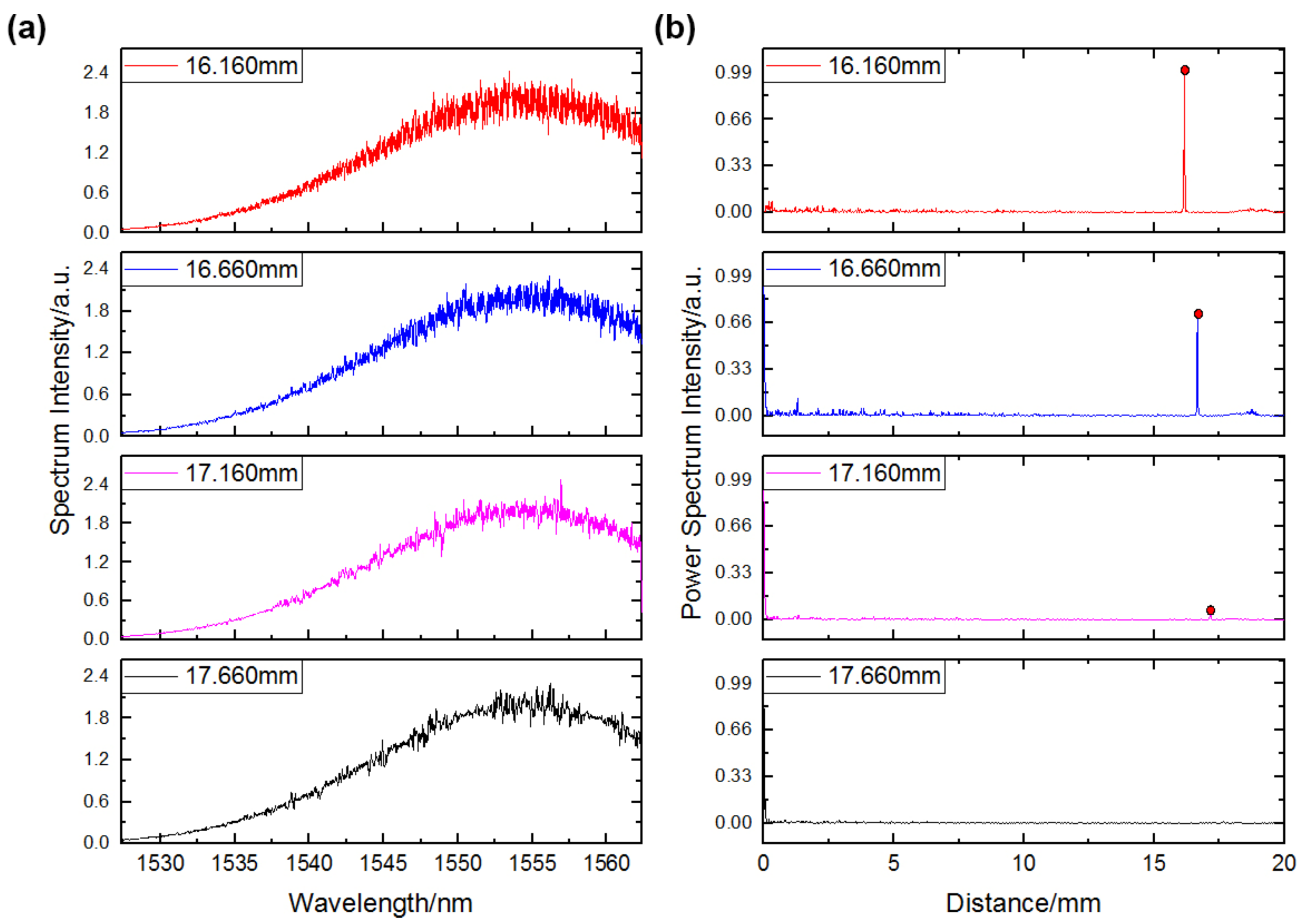
3.2. Measure Range and Accuracy

We evaluated the range of the OFDI system numerically in Matlab. According to Equation (2), the theoretical Dmax was 17.160 mm when λ0 was 1550 nm; therefore, we simulated the OFDI signal at 16.160 mm, 16.660 mm, 17.160 mm, and 17.660 mm. In the simulation, the resolution effect of the FOS was treated as a convolution calculation for the OFDI signal with a two-point rectangular window (approximately two times the FOS sample rate of 0.034 nm). The simulated signals and the power spectrum intensity for the corresponding signals are shown in Figure 5. As shown in Figure 5a, the harmonic characteristics of the signal were difficult to distinguish as the distance increased. The characteristic peak represented the distance that nearly vanished at 17.160 mm and disappeared at 17.660 mm, as shown in Figure 5b. This result verified the theoretical definition of Equation (2).
The experimental result of the linear motion measurement is shown in Figure 6. More than 100 data points were calculated by DFT in each position, and the statistical mean was treated as the measured distance. The range and linearity were evaluated using the method mentioned in our previous work [22]. The OFDI could measure the absolute distance from 1.171 mm to 5.726 mm with a range of 4.555 mm. The accuracy was 0.006 mm, and the calculated linearity was 0.13%. The theoretical Dmax was approximately 3.8 times longer than the experimental result. This resulted from the detailed fuzzying of the signal induced by the accumulated background noise in the integrated time of the detector.

3.3. Vibration Measurement

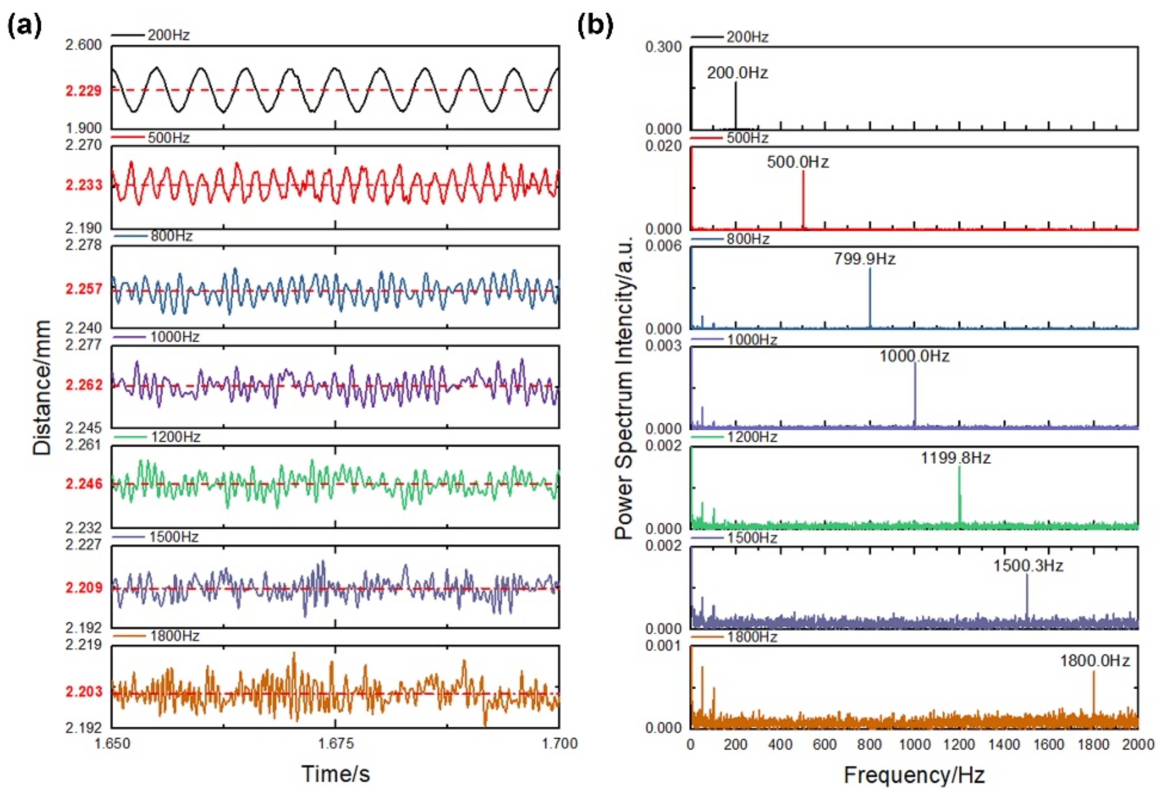
3.3.1. Harmonic Excitation

Harmonic excitation experiments were implemented to verify the vibration measurement performance of the proposed system. In the experiments, the EVE was driven under harmonic excitation produced by the AFG with frequencies ranging from 200 Hz to 1800 Hz. Meanwhile, the driving voltage was set to be constant at each frequency. The vibration process represented by the dynamic distance under an excitation frequency of 200 Hz is depicted in Figure 7. The whole vibration process lasted 2.958 s and displayed the following four characteristic phases: (1) the resting phase, in which the target on the EVE remained still; (2) the transient phase, in which the motion of the target was combined with damping and forced vibrations; (3) stable vibrating, in which the damping vibration vanished and the target was under pure forced vibration; (4) the attenuating phase, in which the power of AFG was shut down and the target was under damping free vibration which stopped at the end.
The motion in the stable vibrating phase attracted a lot of attention for analyzing the vibration modal. The details of the stable vibrating phase under excitation frequencies of 200 Hz, 500 Hz, 800 Hz, 1000 Hz, 1200 Hz, 1500 Hz, and 1800 Hz are shown in Figure 8a. We statistically analyzed the data throughout the stable vibrating phase and utilized the mean value to represent the equilibrium position (marked in red characters). A Fast Fourier transform (FFT) was employed to achieve the power spectrum intensity of the vibrations under each excitation frequency, as shown in Figure 8b. In the power spectrum, the characteristic peaks, which represented the response frequency of the target, were evident. They were, respectively, distributed at 200.0 Hz, 500.0 Hz, 799.9 Hz, 1000.0 Hz, 1199.8 Hz, 1550.3 Hz, and 1800.0 Hz. The maximum deviation from the set excitation frequency was 0.3 Hz.
We could employ the vibration amplitude under different excitation frequencies to fit the vibration parameter. In the transient phase, the damping coefficient could be ignored, and the amplitude obeyed the relation depicted as follows:
A = F 0 m 1 ω 0 2 ω 2 ,
where A is the vibration amplitude, ω is the excitation circular frequency, F0 is the excitation force, m is the mass of the target, and ω0 is the natural frequency of the target. The value of ω0 was 2π × 36.7 rad/s with a standard deviation of 2π × 0.5 rad/s, which could be calculated by the exponential fitting of the distant peaks of the measured distance curves in the transient and attenuating phases under excitation frequencies of 200 Hz, 1000 Hz, and 1800 Hz. The vibration amplitude was attenuated and ambiguous with the increased frequency of the constant excitation force, especially at a frequency of more than 1000 Hz. Obtaining the root mean square (RMS) directly from a distance curve combined with noise was challenging. Instead, we extracted the characteristic peaks in the power spectrum intensity shown in Figure 8b and fitted them with Equation (3) to obtain the ratio of F0 and m. The result is shown in Figure 9. The peaks analyzed in Figure 8b were 0.173 mm, 0.014 mm, 0.004 mm, 0.002 mm, 0.002 mm, 0.001 mm, and 0.001 mm for each excitation frequency. The fitting ratio of F0/m was 166.6 N/kg, with an R-squared value of 0.991.
Traditional vibration technologies, such as accelerometers or LDV, can only obtain the relative displacement from the measurement origin, which is unknown during tests. As a result, the absolute positional relationship between components in the structure cannot be monitored through the experiment process flow. This drawback could be conquered with the proposed OFDI. Figure 10a displays the distance change in the resting phase under the excitation frequencies under 200 Hz. The OFDI monitored a slight distance fluctuation induced by environmental disturbance during the first 0.379 s. A nine-order polynomial fitting was used to quantify the change and indicated a range of 0.010 mm. Similar to the statistical method mentioned above, the original vibration position could be fixed at a distance of 2.213 mm and calculated by statistically analyzing the mean of all the resting-phase data.
Similarly, we statistically analyzed the original positions in the resting phase and the final standings after the attenuating phase in sequential experiments under different excitation frequencies. Combined with the equilibrium positions analyzed in Figure 8a, the change in the absolute positional relationship between the FP and the target in the experimental process was acquired, as shown in Figure 10b. We found that the origin and final positions were consistent in each experiment, with a maximum deviation of 0.010 mm. However, there were apparent position status changes before the experiment at 800 Hz and after 1200 Hz, with a maximum deviation of 0.049 mm. Furthermore, the equilibrium position presented a significant difference when the vibration started. The maximum displacement was 0.012 mm.

3.3.2. Anharmonic Periodic Excitation

An anharmonic periodic excitation experiment was implemented with the same experimental setup mentioned in Section 3.1. The EVE was driven by an AFG under periodic excitation, with the frequency sweeping from 200 Hz to 2000 Hz in 0.5 s. The driving voltage was not constant because the power amplifier in the EVE had an unequal gain compared to the different exciting frequencies in the sweeping period. The dynamic distance measured by the proposed system is shown in Figure 11a. The process lasted approximately 3.2 s, and five distinct periods were observed.
The measured distance curve details are shown in Figure 11b. The time interval calculated using the start points between the adjacent sweeping periods was identical to the set value. The short-time Fourier transformation (STFT) method was adopted to analyze the frequency conversion in every sweeping period (see Figure 9). The number of window points was 256, the overlap was 100, and the FFT length was 4096. As a result, the time resolution was 28.4 ms, and the frequency resolution was 2.2 Hz. In the scale color image of the STFT power spectrum intensity (in dB, see Figure 11c), the character of the frequency chirp representing the frequency conversion as time was displayed. The maximum distinguishable frequency was 1554.8 Hz. The limitation of a low-excitation-frequency signal length is that it makes the power spectrum intensity vague below 250 Hz. Therefore, we extracted the maximum value above 250 Hz to characterize the response frequency corresponding to each discrete time. The extracted data are shown in Figure 11d. Linear fitting was employed for each sweeping period, and the slope of the fitting line was referred to as the sweeping rate of the chirp. In the five sweeping periods, the fitted slopes were 3580.1 Hz/s ± 13.1 Hz/s, 3599.0 Hz/s ± 6.9 Hz/s, 3580.9 Hz/s ± 17.3 Hz/s, 3591.5 Hz/s ± 11.3 Hz/s, and 3557.9 Hz/s ± 52.8 Hz/s, respectively, with a maximum deviation of 41.1 Hz/s to the set parameter of 3600 Hz/s.

3.4. Comparison Measurement

STFT was employed to extract the velocity curve from the signal of the DISAR in a comparison measurement. In the STFT, the number of window points was 512, the overlap was 300, and the FFT length was 2048. As a result, the time resolution was 0.051 ms. The velocity accuracy of the DISAR is represented by the following equation:
Δ v Δ t = λ N W 2 N F T
where Δv is the velocity resolution, Δt is the window length of the STFT, λ is the center wavelength, and NW and NFT are the number of window points and the FFT length, respectively. According to Equation (4), the velocity resolution of the DISAR was 3.8 mm/s. When constrained by the storage depth of a digital oscilloscope, DISAR can only record a signal lasting 20 ms, and so the comparison was limited to 18 ms after the vibration started. The distance curve under the excitation frequency of 500 Hz is shown in Figure 12a. It displays a similar combination of damping and forced vibrations to those discussed in Section 3.3.1. Notably, in the time range of 4.6 ms–5.8 ms, the measured distance was near the upper measurement limit of 5.726 mm, and so the OFDI signal was readily fuzzy, and the results calculated using DFT were treated as gross errors. This region was marked as the signal loss section (SLS, the cyan rectangle in Figure 12a). Using the differentiation method for the measured distance, we obtained the velocity curve, which is demonstrated by the solid red line in Figure 12b. Compared with that acquired by the DISAR (the blue dash line in Figure 12b), there were distinct deviations in the peaks and valleys of the velocity curve with a maximum of 86 mm/s. The deviations were caused by the noncoincidence of zone illumination by the FP and FFP. When the absolute value of the velocity was smaller than 15 mm/s, the insufficiency of interferometrical fringes in the STFT window gave rise to the vagueness of the power spectrum intensity, and so we could not extract a valid velocity in this region (the dead zone of DISAR) whereby the curve was intermittent. However, using the absolute distance measurement property of the OFDI, we could monitor the continuous velocity change, even if the velocity was nearly zero.

4. Discussion

The presented results show that the presented pulse-train OFDI could realize high-speed motion acquisitions up to 9 kHz. The fuzzy dynamic motion was suppressed by the precise time synchronization of the light pulse ejection and optoelectronic component’s operation in the device; therefore, the OFDI spectrum was distinct. The ranging performance was characterized by a linear motion experiment, and an accuracy of 0.006 mm and a range of 4.555 mm were confirmed.
In the harmonic excitation experiments, the absolute distance changes in the motional target were successfully recorded under excitation frequencies ranging from 200 Hz to 1800 Hz. The whole vibration process experiencing four characteristic phases was observed, and the characteristic parameters representing the vibration could be analyzed from the distance results. The maximum deviation of the measured excitation frequency was only 0.3 Hz. Otherwise, the proposed system could monitor position changes in the sequential experiments under different excitation frequencies, which has not been realized with conventional technologies such as accelerometers or LDV. The dynamic distance curve representing the frequency conversion at the sweeping rate of 3600 Hz/s was acquired in the anharmonic periodic excitation experiment. STFT was used to extract the sweeping rate in five cycles with a maximum deviation of 41.1 Hz/s to set the parameter. Significantly, a comparison experiment with DISAR was illustrated. The results showed that the OFDI had the character of monitoring the continuous velocity change, even if the velocity was nearly zero, in which case the DISAR could not give a valid velocity result.
In these experiments, two typical fiber pins were used as vibration sensors. They are flexible in practical applications and easily implanted into narrow gaps of several millimeters, which is similar to the internal structure modal test environment. Unlike the off-axial interferometric structure of traditional LDV technology, the reference origin was set inside the pins, and so the optical path difference between the reference pulse and signal pulse was only the distance between the end front of the fiber and the target. As a result, perturbations on the fiber link could not disturb the OFDI signal. This advantage allowed the pulse-strain OFDI to record dynamic motion processes in several seconds. In addition, the ability of the high-accuracy absolute distance measurements in the sequential vibration experiments demonstrated great practice application potential for monitoring the positional relationship between components through the assembling, testing, and transporting flow in the experimental process. The estimation of the experimental safety or deviation from the initial design was significant.
In the pulse-strain OFDI system, the line-array detector developed the sample rate more than a traditional OFDI method would. Although the practical range was only 4.555 mm shorter than the theoretical evaluation, this scheme had the potential to realize a larger range without losing accuracy when reducing the background noise of the FOS. The proposed system was constructed of all-fiber, similar to a TOF. Even if the signal record device was a high-optical-resolution FOS, the cost of the system was lower than that of a TOF, which employs a high-bandwidth photodiode and oscilloscope to detect the rapidly rising edge of a photocurrent pulse. Meanwhile, the system was more compact, flexible, and robust compared to a cumbersome and complex camera-type LCI system. It was reliable in complex environments, such as a centrifuge or compound vibration platform. Compared with LCI and traditional OFDI, the inadequacy in accuracy was caused by the limited wavelength accuracy of the FOS and the bandwidth of the OFDI signal. According to the Fourier transformation theory and the power spectrum of the measured signal, the width of the characteristic peak corresponding to the 17 nm signal width was approximately 0.07 mm, which was only represented by three points. The wavelength accuracy could easily affect the intensity of the represented points and increase the error of the signal process. With the development of high-quantum-efficiency near-infrared CMOS detectors and ultra-precision gratings in the future, the accuracy will be prospectively improved and realized in a submicron order. Furthermore, the high insertion loss of the AOM required the high pulse energy of the NPLS, and the heat effect on the target may have reduced the measurement accuracy, especially for low thermal conductivity materials.

Author Contributions

Conceptualization, C.L. (Cangli Liu), J.W. (Jidong Weng), and H.M.; methodology, J.W. (Jidong Weng) and H.M.; validation, H.M., L.C., and T.T.; formal analysis, H.M. and L.C.; investigation, H.M.; resources, X.J.; data curation, S.L.; writing—original draft preparation, H.M.; writing—review and editing, H.M. and L.T.; supervision, X.W.; project administration, J.W. (Jidong Weng); funding acquisition, C.L. (Chengjun Li), J.W. (Jian Wu), and L.T. All authors have read and agreed to the published version of the manuscript.

Funding

This research was funded by the National Natural Science Foundation of China under grant numbers 62101518 and U2241276 and the Foundation of National Key Laboratory of Shock Wave and Detonation Physics under grant number JCKYS2022212001.

Institutional Review Board Statement

Not applicable.

Informed Consent Statement

Not applicable.

Data Availability Statement

The data are contained within the article.

Conflicts of Interest

The authors declare no conflict of interest.

References

  1. Rana, K. Fuzzy control of an electrodynamic shaker for automotive and aerospace vibration testing. Expert Syst. Appl. 2011, 38, 11335–11346. [Google Scholar] [CrossRef]
  2. Brown, R.; Singh, K.; Khan, F. Fabrication and vibration characterization of electrically triggered shape memory polymer beams. Polym. Test 2017, 61, 74–82. [Google Scholar] [CrossRef]
  3. Amorebieta, J.; Ortega-Gomez, A.; Durana, G.; Fernández, R.; Antonio-Lopez, E.; Schülzgen, A.; Zubia, J.; Amezcua-Correa, R.; Villatoro, J. Highly sensitive multicore fiber accelerometer for low frequency vibration sensing. Sci. Rep. 2020, 10, 16180. [Google Scholar] [CrossRef] [PubMed]
  4. Zhang, P.; Wang, S.; Jiang, J.; Li, Z.; Yang, H.; Liu, T. A fiber-optic accelerometer based on extrinsic Fabry-Perot interference for low frequency micro-vibration measurement. IEEE Photonics J. 2022, 14, 1–6. [Google Scholar] [CrossRef]
  5. Wang, W.C.; Hwang, C.H.; Lin, S.Y. Vibration measurement by the time-averaged electronic speckle pattern interferometry methods. Appl. Opt. 1996, 35, 4502–4509. [Google Scholar] [CrossRef] [PubMed]
  6. Bhaduri, B.; Mohan, N.K.; Kothiyal, M.P.; Sirohi, R.S. Use of spatial phase shifting technique in digital speckle pattern interferometry (DSPI) and digital shearography (DS). Opt. Exp. 2006, 14, 11598–11607. [Google Scholar] [CrossRef]
  7. Sheng, Z.; Chen, B.; Hu, W.; Yan, K.; Miao, H.; Zhang, Q.; Yu, Q.; Fu, Y. LDV-induced stroboscopic digital image correlation for high spatial resolution vibration measurement. Opt. Exp. 2021, 29, 28134–28147. [Google Scholar] [CrossRef] [PubMed]
  8. Pedrini, G.; Osten, W.; Gusev, M.E. High-speed digital holographic interferometry for vibration measurement. Appl. Opt. 2006, 45, 3456–3462. [Google Scholar] [CrossRef]
  9. Na, Y.; Jeon, C.-G.; Ahn, C.; Hyun, M.; Kwon, D.; Shin, J.; Kim, J. Ultrafast, sub-nanometre-precision and multifunctional time-of-flight detection. Nat. Photonics 2020, 14, 355–360. [Google Scholar] [CrossRef]
  10. Wojtkowski, M.; Kowalczyk, A.; Leitgeb, R.; Fercher, A.F. Full range complex spectral optical coherence tomography technique in eye imaging. Opt. Lett. 2002, 27, 1415–1417. [Google Scholar] [CrossRef]
  11. Sun, X.; Feng, K.; Cui, J.; Dang, H.; Niu, Y.; Zhang, X. A micro absolute distance measurement method based on dispersion compensated polarized low-coherence interferometry. Sensors 2020, 20, 1168. [Google Scholar] [CrossRef]
  12. Cusato, L.J.; Cerrotta, S.; Torga, J.R.; Morel, E.N. Extending low-coherence interferometry dynamic range using heterodyne detection. Opt. Laser Eng. 2020, 131, 106106. [Google Scholar] [CrossRef]
  13. Rothberg, S.J.; Allen, M.S.; Castellini, P.; Di Maio, D.; Dirckx, J.J.J.; Ewins, D.J.; Halkon, B.J.; Muyshondt, P.; Paone, N.; Ryan, T.; et al. An international review of laser Doppler vibrometry: Making light work of vibration measurement. Opt. Lasers Eng. 2016, 99, 11–22. [Google Scholar] [CrossRef]
  14. Castellini, P.; Martarelli, M.; Tomasini, E.P. Laser Doppler Vibrometry: Development of advanced solutions answering to technology’s needs. Mech. Syst. Signal Process. 2006, 20, 1265–1285. [Google Scholar] [CrossRef]
  15. Heydemann, P.L.M. Determination and correction of quadrature fringe measurement errors in interferometers. Appl. Opt. 1981, 20, 3382–3384. [Google Scholar] [CrossRef] [PubMed]
  16. Park, S.; Lee, J.; Kim, Y.; Lee, B.H. Nanometer-Scale Vibration Measurement Using an Optical Quadrature Interferometer based on 3 × 3 Fiber-Optic Coupler. Sensors 2020, 20, 2665. [Google Scholar] [CrossRef]
  17. Shang, J.; He, Y.; Wang, Q.; Li, Y.; Ren, L. Development of a High-Resolution All-Fiber Homodyne Laser Doppler Vibrometer. Sensors 2020, 20, 5801. [Google Scholar] [CrossRef] [PubMed]
  18. Mandel, L.; Wolf, E. Spectral coherence and the concept of cross-spectral purity. J. Opt. Soc. Am. 1976, 66, 529–535. [Google Scholar] [CrossRef]
  19. Gahagan, K.T.; Moore, D.S.; Funk, D.J.; Rabie, R.L.; Buelow, S.J.; Nicholson, J.W. Measurement of shock wave rise times in metal thin film. Phys. Rev. Lett. 2000, 85, 3205–3208. [Google Scholar] [CrossRef] [PubMed]
  20. Weng, J.; Tao, T.; Liu, S.; Ma, H.; Wang, X.; Liu, C.; Tan, H. Optical-fiber frequency domain interferometer with nanometer resolution and centimeter measuring range. Rev. Sci. Instrum. 2013, 84, 113103. [Google Scholar] [CrossRef]
  21. Weng, J.D.; Hua, T.; Wang, X.; Ma, Y.; Hu, S.L.; Wang, X.S. Optical-fiber interferometer for velocity measurements with picosecond resolution. Appl. Phys. Lett. 2006, 89, 4669. [Google Scholar] [CrossRef]
  22. Ma, H.; Liu, S.; Tao, T.; Chen, L.; Tang, L.; Li, C.; Wu, J.; Jia, X.; Wang, X.; Weng, J. A high-performance ranging method with a long distance range and high accuracy. Optik 2022, 253, 168526. [Google Scholar] [CrossRef]
Figure 1. (a) Schematic of the proposed pulse-train OFDI. NPLS, nanosecond pulsed light source; FC, fiber circulator; FP, fiber pin; EVE, electro-vibration exciter; DDG, digital delay generator; AOM, acousto-optic modulator; AFG, arbitrary waveform generator; P-EDFA, pulsed erbium-doped fiber amplifier; FOS, fiber-optic spectrometer. (b) Photograph of the department combined with the EVE, target, and FP. (c) Photograph of the FP.
Photonics 10 01342 g001
Figure 2. Setup of the linear motion measurement experiment.
Photonics 10 01342 g002
Figure 3. (a) Setup of the comparison experiment. (b) Photograph of the FFP.
Photonics 10 01342 g003
Figure 4. (a) Typical OFDI signal recorded by an FOS. (b) Time synchronization signals of the proposed system.
Photonics 10 01342 g004
Figure 5. (a) The simulated OFDI signals at 16.160 mm, 16.660 mm, 17.160 mm, and 17.660 mm. (b) The power spectrum intensity corresponding to each distance.
Photonics 10 01342 g005
Figure 6. Experimental results.
Photonics 10 01342 g006
Figure 7. The vibration process at an excitation frequency of 200 Hz.
Photonics 10 01342 g007
Figure 8. (a) Details of the stable vibrating phase under different excitation frequencies. (b) The power spectrum intensity corresponding to each excitation frequency.
Photonics 10 01342 g008
Figure 9. The extracted peaks from the power spectrum intensity and the fitting line using the amplitude function indicated in Equation (3).
Photonics 10 01342 g009
Figure 10. (a) Distance details in the resting phase under an excitation frequency of 200 Hz. (b) The origin, equilibrium, and final positions after the attenuating phase of the sequential experiments.
Photonics 10 01342 g010
Figure 11. (a) Measured dynamic distance under the excitation frequency sweeping from 200 Hz to 2000 Hz in 0.5 s. (b) Details of the results. (c) Scale color image of the STFT power spectrum intensity. (d) Linear fitting of the extracted frequency value.
Photonics 10 01342 g011
Figure 12. (a) Results of the measured distance under the excitation frequency of 500 Hz. (b) Velocity comparison between the STFT calculated result of the DISAR and the differential from the measured distance by the proposed OFDI.
Photonics 10 01342 g012
Disclaimer/Publisher’s Note: The statements, opinions and data contained in all publications are solely those of the individual author(s) and contributor(s) and not of MDPI and/or the editor(s). MDPI and/or the editor(s) disclaim responsibility for any injury to people or property resulting from any ideas, methods, instructions or products referred to in the content.

