Article

An Angle Precision Evaluation Method of Rotary Laser Scanning Measurement Systems with a High-Precision Turntable

State Key Laboratory of Precision Measuring Technology and Instruments, Tianjin University, Tianjin 300072, China
*
Author to whom correspondence should be addressed.
Photonics 2023, 10(11), 1224; https://doi.org/10.3390/photonics10111224
Submission received: 30 September 2023 / Revised: 20 October 2023 / Accepted: 26 October 2023 / Published: 1 November 2023
(This article belongs to the Special Issue Optical Measurement Systems)

Abstract

:
Rotary laser scanning measurement systems, such as the workshop measurement positioning system (wMPS), play critical roles in manufacturing industries. The wMPS realizes coordinate measurement through the intersection of multiple rotating fanned lasers. The measurement model of multi-laser plane intersection poses challenges in terms of accurately evaluating the system, making it difficult to establish a standardized evaluation method. The traditional evaluation method is based on horizontal and vertical angles derived from scanning angles, which are the direct observation of wMPS. However, the horizontal- and vertical-angle-based methods ignore the assembly errors of fanned laser devices and mechanical shafts. These errors introduce calculation errors and affect the accuracy of angle measurement evaluation. This work proposes a performance evaluation method for the scanning angle independent of the assembly errors above. The transmitter of the wMPS is installed on a high-precision turntable that provides the angle reference. The coordinates of enhanced reference points (ERP) distributed in the calibration space are measured by the laser tracker multilateration method. Then, the spatial relationship between the transmitter and the turntable is reconstructed based on the high-precision turntable and the good rotational repeatability of the transmitter. The simulation was carried out to validate the proposed method. We also studied the effect of fanned laser devices and shaft assembly errors on horizontal and vertical angles. Subsequently, the calibration results were validated by comparing the residuals with those derived from the space-resection method. Furthermore, the method was also validated by comparing the reference and scanning angles. The results show that the maximum angle measurement error was approximately 2.79″, while the average angle measurement error was approximately 1.26″. The uncertainty (k = 1) of the scanning angle was approximately 1.7″. Finally, the coordinate measurement test was carried out to verify the proposed method by laser tracker. The results show that the average re-scanning error was 2.17″.

1. Introduction

Rotary laser scanning measurement systems, represented by a workshop measurement positioning system (wMPS) and an indoor global positioning system (iGPS), play a vital role in many manufacturing industries due to their excellent full-circumference and parallel multi-target measurement capabilities [1,2,3,4,5,6]. However, the complicated environment, involving vibration and temperature changes in industrial sites, has a significant influence on the mechanical structure of the wMPS transmitters and further degrades the measurement performance over time. In addition, the large measurement volume and the complex error propagation law in the wMPS network make it difficult to maintain accuracy. Therefore, performance evaluation is critical to ensure traceable and reliable results.
A measurement network comprises three parts: transmitters, receivers, and signal processors. The rotating head of each transmitter emits two fanned laser beams and a strobe to stimulate the receivers. The receiver detects and recognizes the laser signals when the signals arrive. Signal processors calculate the scanning angle between the transmitter and the receiver by the transmitter’s rotation speed and the arrival time of different signals. The traditional angle-based measurement models, which calculate horizontal and vertical angles by scanning angles and the normal vectors of fanned lasers, are widely used [7,8]. However, the traditional method ignores the assembly errors of fanned laser devices and mechanical shafts, causing calculation errors and decreasing the effectiveness of the performance evaluation method.
As shown in Figure 1, traditional measurement models ignore the effects of laser devices and shaft assembly errors, which are inevitable during production. Many performance evaluation methods based on traditional models have been proposed. Muelaner et al. presented a study on the uncertainty of angle measurement based on traditional models [7]. Zhao et al. improved this method by introducing an evaluation of vertical angles calculated using traditional measurement models [8]. Because assembly errors significantly influence measurement accuracy, the angle evaluation methods are flawed.
Because of the intractable assembly error, several works have been published only to evaluate performance from integrated measurement systems or mechanical properties. Qiang et al. presented research on the device error and its influence on positioning accuracy in iGPS [9]. Muelaner et al. presented an uncertainty estimation method of three-dimensional coordinates for iGPS [10]. R. Schmitt et al. presented a performance evaluation method of iGPS for industrial applications [11]. Su et al. presented a space-resection method to calibrate the rotary laser scanning measurement systems and analyze the precision of calibration [12]. Because of the strong coupling relationship between the coordinate and the scanning angle, these methods cannot reflect the actual performance of the single transmitter, so a reasonable evaluation target is urgently needed in order to evaluate the transmitter.
Similar problems also arise regarding the performance evaluation of the laser tracker. The horizontal and vertical angles model is unable to express the error of encoders accurately because of the assembly error. The ASME B89.4.19 standard has been established for the performance evaluation of the laser tracker. This standard focuses on the integrated measurement system [13]. Meanwhile, many researchers have invested their effort in verifying the performance of laser trackers’ isolating subsystems by parameterizing assembly errors. Hughes et al. proposed a method to determine the geometrical alignment errors of a laser tracker using a network measurement [14]. O Icasio-Hernández et al. evaluated the uncertainty and improved the geometry error parameters of a laser tracker using the network method [15]. Wang et al. improved this method by introducing reference lengths derived by optimization [16]. These evaluation methods parameterize assembly error and use direct observations to achieve error separation.
The multi-plane, constraint-based measurement model is proposed to parameterize the assembly error, and it is more consistent with the physical structure of the transmitter. In this model, the scanning angle is the direct observation that is not associated with system parameters. Therefore, it is reasonable to choose the scanning angle as the target of performance evaluation to achieve error separation. The error introduced in the calibration process and the influence of assembly error are suppressed by introducing the scanning angle. The proposed method evaluates the scanning angle with a high-precision turntable to increase the precision of the evaluation. This method relies on the reference angle and the good rotational repeatability of transmitters, which ensure the accuracy of performance evaluation. In addition, a high-precision calibration method is proposed to establish a relationship between the turntable and the transmitter to avoid manual adjustment of the concentricity and parallelism.
The proposed method involves the following three steps. First, a laser tracker is used to construct the enhanced reference points (ERP). The laser tracker measures the ERP in separate locations, and the measurement results of laser trackers are optimized by, redundantly, Laser Interferometer Measurement [17]. Second, the transmitter is fixed on a turntable, and we verify the rotational repeatability of the transmitter. An averaging algorithm is applied to further decrease the repeatability error. Third, the turntable is operated to make the transmitter’s observations for each control point the same. The target function is established to calibrate the relationship between the transmitter and the turntable, and the Levenberg–Marquardt algorithm is utilized [18]. Finally, the evaluation results are derived by comparing the reference and scanning angles.
The rest of the study is organized as follows. In Section 2, we introduce the measurement model of the wMPS and the corresponding mathematical models of the turntable and transmitter system. Additionally, the method establishes the evaluation reference and evaluates the performance of the scanning angle measurement. Monte Carlo simulations are used to verify the proposed method in Section 3. The experimental setup and results of the evaluation of the transmitter’s scanning angle error are presented in Section 4. Finally, the conclusions and our future work are presented in Section 5.

2. Measurement Model and Error Analysis of wMPS

The multi-plane, constraint-based measurement model and definition of the scanning angle are described in Section 2.1. In addition, the effects of assembly error on vertical and horizontal angles are also indicated in Section 2.1. To establish a relationship between the scanning angle and the reference angle, a calibration method is presented in Section 2.2. Furthermore, an evaluation method is proposed to estimate the scanning angle error at different positions in Section 2.3.

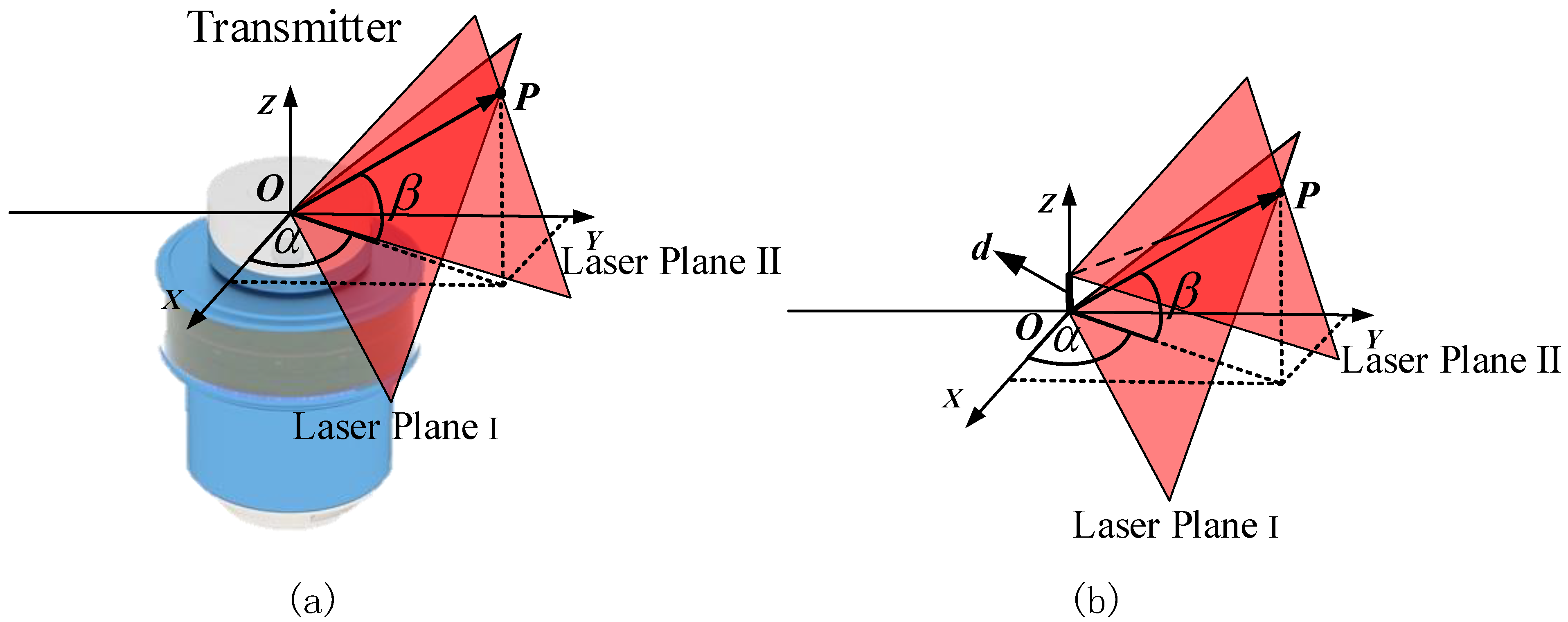
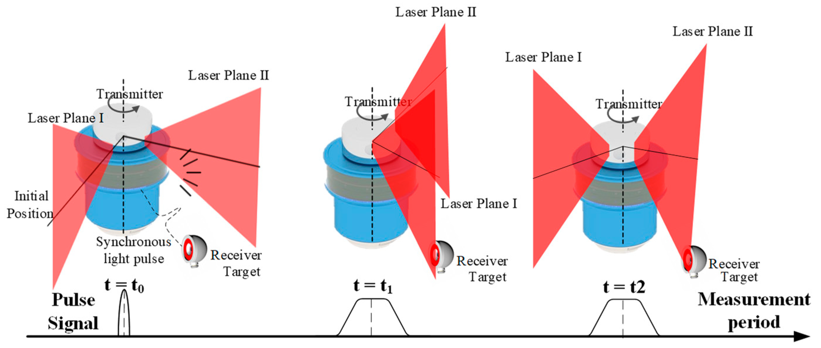
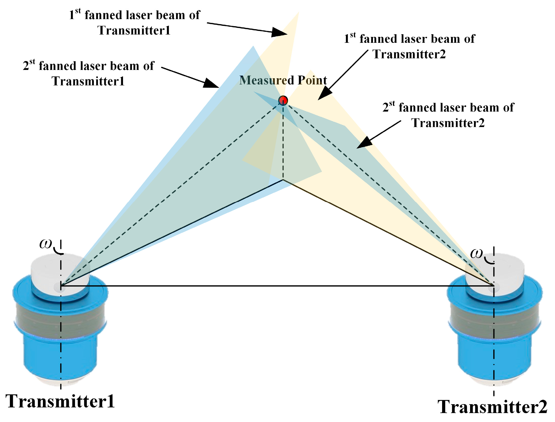
2.1. Measuring Principle of wMPS

The wMPS is based on rotary-laser scanning, which can precisely convert three-dimensional coordinates into two scanning angles. It consists of two or more transmitters, several receivers, and data process systems. Each transmitter contains a fixed base, a rotating head with two fanned laser devices, and a ring laser device that generates a 360° strobe. The receiver consists of a spherical shell with a 38.1 mm (1.5 in) diameter, a photoelectric sensor to receive the laser signals, and cables connected to the data process system. The data process system contains a wireless signal processor that can convert a light signal to a digital signal, a router to connect wireless processors, and a portable computer [8].
The measuring principle of transmitters is to calculate the scanning angle through the time difference generated by fanned-laser rotation. As shown in Figure 2, the transmitter’s head rotated at a stable, high speed and marks the beginning of each lap using an encoder. The ring laser device generated a synchronous strobe at the beginning of each lap. The time at which the receivers detected the synchronous strobe was recorded as the initial time t 0 . When the receiver detected two light signals from two rotating fanned lasers, those times were recorded as t 1 and t 2 . The transmitters’ signal and time data for each lap were sent to the data processor. Because each transmitter rotated at a given speed, the measurement periods T i of all transmitters were different. Hence, the signal from each transmitter was extracted separately.
As shown in Figure 3, the scanning angle was derived from each transmitter’s time signal by the equation θ 1 = 2 π ( t 1 t 0 ) / T , θ 1 = 2 π ( t 2 t 0 ) / T , where θ 1 and θ 2 represent the corresponding scanning angles when the receiver detects the signal from the first and second fanned laser beams, respectively.
In the transmitter’s local coordinate system, the Z-axis is typically the rotation axis of the rotating head. Furthermore, the intersection point between the first laser beam and the Z-axis is the origin. The direction of the encoder’s zero point is the X-axis, and the Y-axis is determined according to the right-hand rule.
Combined with the plane parameter a 1 , b 1 , c 1 , a 2 , b 2 , c 2 and the extrinsic parameters, the relationship between the receiver and transmitter can be solved by Equation (1):
{ [ a 1 b 1 c 1 ] [ cos ( θ 1 ) sin ( θ 1 ) 0 sin ( θ 1 ) cos ( θ 1 ) 0 0 0 1 ] ( [ R 1 R 2 R 3 R 4 R 5 R 6 R 7 R 8 R 9 ] [ X Y Z ] + [ T X T Y T Z ] ) = 0 [ a 2 b 2 c 2 ] [ cos ( θ 2 ) sin ( θ 2 ) 0 sin ( θ 2 ) cos ( θ 2 ) 0 0 0 1 ] ( [ R 1 R 2 R 3 R 4 R 5 R 6 R 7 R 8 R 9 ] [ X Y Z ] + [ T X T Y T Z ] ) = d
In this function, d is the deviation between the two laser devices along axis Z, which is caused by assembly error. d is usually on the order of the millimeter level and has a non-negligible effect on the measurement results [19]. While the scanning angles θ 1 and θ 2 are independent of d , the coordinates of the measured points are influenced by the deviation d and further affect the horizontal and vertical angles.
As shown in Figure 4, each wMPS usually consists of two or more transmitters. And the coordinate of the measured point is derived from the intersection of the laser plane emitted by the transmitter. Thus, the measurement function can be derived by Equation (2):
A [ X Y Z ] = δ
A is a 2n × 3 array, and each row for A is expressed as Equation (3):
A ( i 1 ) * 2 + k = [ a ik b ik c ik ] [ cos ( θ ik ) sin ( θ ik ) 0 sin ( θ ik ) cos ( θ ik ) 0 0 0 1 ] [ R i 1 R i 2 R i 3 R i 4 R i 5 R i 6 R i 7 R i 8 R i 9 ]
δ is a 2n vector, and each element is expressed as Equation (4):
δ ( i 1 ) * 2 + k = [ a ik b ik c ik ] [ cos ( θ ik ) sin ( θ ik ) 0 sin ( θ ik ) cos ( θ ik ) 0 0 0 1 ] [ T i X T i Y T i Z ] d ik
The following Equation (5) can derive the point’s 3D coordinate:
[ X Y Z ] = ( A T A ) 1 A T δ

2.2. The Effect of Assembly Error on Vertical and Horizontal Angle

According to the measurement principle, the scanning angle was not related to the parameter d , which was introduced by the assembly error. Hence, the described measurement model was suitable for evaluation, and the scanning angle was the reasonable evaluation object.
In the traditional measurement model, the horizontal and vertical angles are directly associated with the distance between the target and transmitter because of assembly errors d , and is coupled with the normal vector of fanned lasers. The simulation is applied to analyze the effect of distance between the target and transmitter on horizontal and vertical angles when d equals 1 mm.
The simulation results are shown in Figure 5 and Figure 6. The horizontal and vertical angle errors introduced by laser devices and shaft assembly errors varied with the distance between the target and transmitter, and the introduced error was significant. The simulation results indicate that the evaluation method based on the horizontal and vertical angles was not accurate. The accuracy of the horizontal and vertical angles changed as the target changed. The farther the target was from the transmitter, the smaller the error became, but there was still an error of more than 10 arc seconds in the main working distance of the transmitter. Thus, it was necessary to select the scanning angle as the evaluation target to reflect the actual performance of the transmitters.

2.3. Establishment of the Evaluation Reference

The process of introducing a reference angle is necessary in order to evaluate the scanning angle measurement’s performance. A high-precision turntable is an instrument that can provide high-precision angle reference and has a high angular resolution. When the turntable is selected as the angle reference of the transmitter, the relationship between the turntable and the transmitter needs to be carefully calibrated. However, it is difficult to calibrate the relationship between the transmitter and the turntable accurately by the space resection method because of the angle measurement error of wMPS. Therefore, the calibration method of the relationship between the transmitter and the turntable needs to be improved first.
In the proposed method, the transmitter is installed on the turntable using a connector to ensure the approximate alignment of the rotary axis transmitter and the turntable. The ERP consisting of several points is arranged in the calibration space. The laser tracker is relocated to multiple positions, and the high-accuracy laser interferometer measurement results are used to improve the accuracy of the ERP by the length measurement results of the laser tracker. The calibration accuracy of the process is better than that obtained using a single laser tracker.
As shown in Figure 7, three Cartesian coordinate systems were defined: the ERP coordinate system O c x c y c z c ( C c ) , the turntable coordinate system O r x r y r z r ( C r ) , and the transmitter coordinate system O t x t y t z t ( C t ) . The rotation and translation matrices from the ERP coordinate system to the transmitter coordinate system were defined as R c t and T c t , respectively. The rotation and translation matrices from the transmitter coordinate system to the turntable coordinate system were defined as R t r and T t r , respectively. Thus, Equation (6) was obtained:
{ R c r = R t r R c t T c r = R t r T c t + T t r
R c t and   T c t are the rotation and translation matrices from the ERP coordinate system to the turntable coordinate system, respectively.
The control point coordinate P c under the ERP coordinate system can be transformed to P t under the transmitter field coordinate system and P r under the turntable coordinate system using Equation (7):
{ P t = R c t   P c + T c t P r = R c r   P c + T c r
Further, the classic wMPS transmitter measurement formula can be represented by Equation (8):
{ n 1 R z ( θ 1 ) P t = 0 n 2 R z ( θ 2 ) P t = d
In this expression, n 1 represents the normal vector of the first fanned laser, n 2 represents the normal vector of the second fanned laser, θ 1 is the scanning angle of the first fanned laser, θ 2 is the scanning angle of the second fanned laser, and d is the intercept for the second fanned laser on axis Z.
When the turntable revolves around the Z-axis, the point coordinate under the turntable coordinate system is given by Equation (9):
P r α = R z ( α ) P r = R z ( α ) ( R c r   P c + T c r )
In this expression, α is the rotation angle of the turntable.
According to Equations (8) and (9), the transmitter measurement model considering the turntable rotation can be given by the following Equation (10):
{ n 1 R z ( θ 1 ) ( R r t ( R z ( α ) ( R c r   P c + T c r ) ) + T r t ) = 0 n 2 R z ( θ 2 ) ( R r t ( R z ( α ) ( R c r   P c + T c r ) ) + T r t ) = d
n 1 , n 2 , R r t , R c r , T c r , T r t and d are the constant matrices, and P c does not change for the same ERP.
The following Equation (11) can be derived from Equation (10):
{ [ a 1 b 1 c 1 ] [ cos ( θ 1 ) sin ( θ 1 ) 0 sin ( θ 1 ) cos ( θ 1 ) 0 0 0 1 ] [ X t Y t Z t ] = 0 [ a 2 b 2 c 2 ] [ cos ( θ 2 ) sin ( θ 2 ) 0 sin ( θ 2 ) cos ( θ 2 ) 0 0 0 1 ] [ X t Y t Z t ] = d
And P T = [ X t Y t Z t ] = ( R r t ( R z ( α ) ( R c r   P c + T c r ) ) + T r t ) .
The transmitter measurement equation can be expressed as Equation (12):
{ ( a 1 X t + b 1 Y t ) cos ( θ 1 ) + ( b 1 X t a 1 Y ) sin ( θ 1 ) + c 1 Z t = 0 ( a 2 X t + b 2 Y t ) cos ( θ 2 ) + ( b 2 X t a 2 Y ) sin ( θ 2 ) + c 1 Z t = d
The complete form of the equation can be expressed as Equation (13):
{ a 1 X t + b 1 Y t ( a 1 X t + b 1 Y t ) 2 + ( b 1 X t a 1 Y t ) 2 cos ( θ 1 ) + ( b 1 X t a 1 Y ) ( a 1 X t + b 1 Y t ) 2 + ( b 1 X t a 1 Y t ) 2 sin ( θ 1 ) = c 1 Z t ( a 1 X t + b 1 Y t ) 2 + ( b 1 X t a 1 Y t ) 2 a 2 X t + b 2 Y t ( a 2 X t + b 1 Y t ) 2 + ( b 2 X t a 2 Y t ) 2 cos ( θ 2 ) + ( b 2 X t a 2 Y ) ( a 2 X t + b 2 Y T ) 2 + ( b 2 X t a 2 Y t ) 2 sin ( θ 2 ) = c 2 Z t + d ( a 2 X t + b 1 Y t ) 2 + ( b 2 X t a 2 Y t ) 2  
θ 1 , θ 2 change when the value of α changes, and Equation (14) represents the corresponding relationship:
{ θ 1 = arcsin r c s i n ( c 1 Z t ( a 1 X t + b 1 Y t ) 2 + ( b 1 X t a 1 Y t ) 2 ) arcsin ( a 1 X t + b 1 Y t ( a 1 X t + b 1 Y t ) 2 + ( b 1 X t a 1 Y t ) 2 ) θ 2 = arcsin ( c 2 Z t + d ( a 2 X t + b 1 Y t ) 2 + ( b 2 X t a 2 Y t ) 2 ) arcsin ( a 2 X t + b 2 Y t ( a 2 X t + b 1 Y t ) 2 + ( b 2 X t a 2 Y t ) 2 )
It is noteworthy that the parameters can be solved by changing the rotation degree. In the traditional method, the relationship between the transmitter and turntable calibrated by this function has low precision because of the scanning angle errors and the distortion of the fanned laser beam. In this study, the distortion of the fanned laser could be suppressed by choosing the appropriate ERP in the proper distribution space. The scanning angle error was mainly determined by the repeatability of the angle measurement, which was easier to verify.
The schematic of turntable adjustment is shown in Figure 8, and the process is illustrated in Figure 9. As shown in Figure 8, the proposed method transformed the angle measurement error into repeatability by choosing a fixed value for the scanning angle. The turntable’s reference angle α was obtained when the value of θ 1 and θ 2 equaled the preset angle. Because the angular resolution of the turntable was less than 0.5 arc seconds, the θ 1 and θ 2 uncertainty for each control point could be reduced to the same level by the mapping relationship. To simplify the expressions, the values of θ 1 and θ 2 were set to π , and Equation (15) was derived.
{ n 1 ( R r t ( R z ( α ) ( R c r   P c + T c r ) ) + T r t ) = 0 n 2 ( R r t ( R z ( α ) ( R c r   P c + T c r ) ) + T r t ) = d
In this equation, n 1 = n 1 [ 1 0 0 0 1 0 0 0 0 ] and n 2 = n 2 [ 1 0 0 0 1 0 0 0 0 ] .
{ n 1 R z ( α ) ( R c r   P c + T c r ) = d 1 n 2 R z ( α ) ( R c r   P c + T c r ) = d 2
In Equation (16), n 1 = n 1 R r t , n 2 = n 2 R r t , d 1 = n 1 T r t , d 2 = n 2 T r t + d . Moreover, Equation (15) is similar to Equation (8), but the uncertainty of α is lower than the uncertainty of the scanning angle, increasing the calibration precision.
The Levenberg–Marquardt algorithm was applied to solve nonlinear equations, and Equation (14) was used as the objective function. The normal vector n 1 had one degree of freedom. R r t and R c r had three degrees of freedom for the rotation along three axes. T r t , T c r   had three degrees of freedom for the translation along three axes. n 2 had two degrees of freedom. d had one degree of freedom. Therefore, this nonlinear optimization problem could be solved if sixteen or more constraint functions were constructed. Alternatively, the number of ERPs should be higher than eight, because each point will introduce two constraints.
The initial values of R c t and T c t were derived by the resection method, and the rotation matrix from the turntable to the transmitter R r t was considered an identity matrix. The translation matrix from the turntable to the transmitter T r t   was considered a zero vector because the rotary axis of the transmitter was nearly the same as the turntable. Then, the Levenberg–Marquardt algorithm was applied to solve the objective function.
The scanning angle measurement error was analyzed by the reference angle expressed as Equation (17):
{ n 1 R z ( θ r e f ) ( R r t ( R z ( α ) ( R c r   P c + T c r ) ) + T r t ) = 0 n 2 R z ( θ r e f ) ( R r t ( R z ( α ) ( R c r   P c + T c r ) ) + T r t ) = d
In this equation, n 1 , R r t , R c r , P c , T c r , T r t and d were known by the calibration progress and ERP. The turntable reference angle α was obtained from the turntable, and the calculated scanning angle θ r e f was derived by the least-square method.
According to the measurement principle of wMPS, the measurement error of θ 1 equals the measurement error of θ 2 . Thus, the measurement error of θ 1 was selected to evaluate the performance of wMPS. The difference Δ θ 1 between the calculated scanning angle θ r e f and the measured scanning angle θ 1 represented the error, expressed as: Δ θ 1 = θ 1 θ r e f .

3. Simulations and Analysis
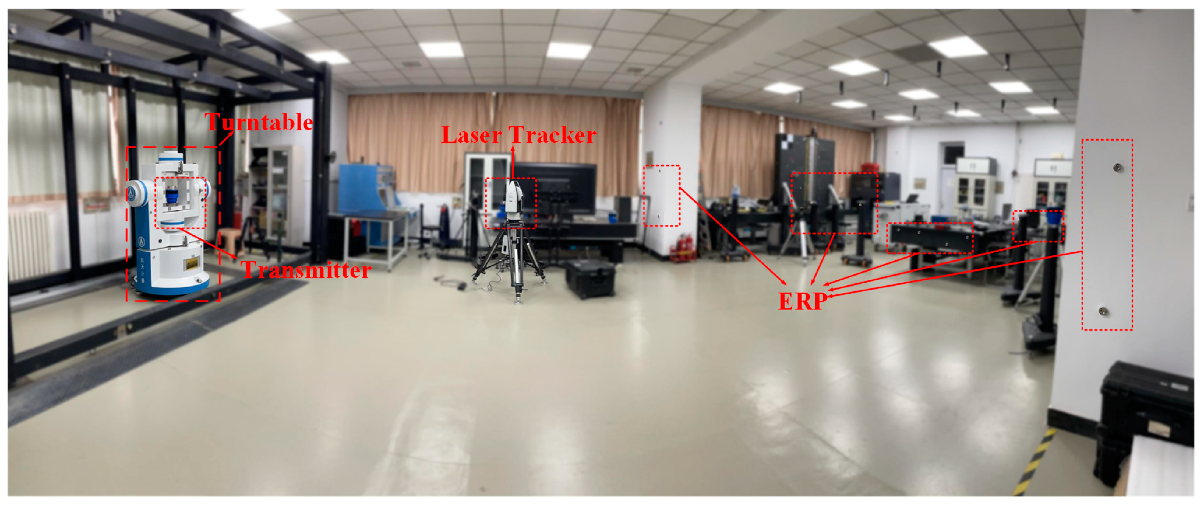
The effectiveness of the scanning angle evaluation is directly associated with cali-bration accuracy. The Monte Carlo simulation and related theoretical analysis are ap-plied to analyze the calibration accuracy.
In this simulation, the rotation matrix R r t from the turntable to the transmitter was represented by three Euler angles. The translation vector T r t from the turntable to the transmitter was represented by the translations along three axes. The angle measurement uncertainty of the turntable was 0.5 arc seconds. The control point’s coordinate measurement uncertainty was 0.02 mm. In addition, 16 ERPs were selected in compliance with the actual experiment. The repeatability error of the transmitter was 0.1 arc seconds. We compared the result of the space-resection calibration method and the method proposed in this article by means of the Monte Carlo simulation.
The result of the simulation is shown in Figure 10. According to the objective function of the space-resection calibration method and the proposed method, the calibration residual of each function was determined by control point restrictions. According to Equation (18), the calibration residual revealed the calibration quality directly for the space-resection method, while Equation (15) reflected the calibration quality for the proposed method. The physical meanings of the two equations were similar, and represented the distance from the control point to the measurement vector formed by the two fanned lasers.
D n = i = 1 2 ( [ a i   b i   c i     d i ] [ cos ( θ n i ) sin ( θ n i ) 0 0 sin ( θ n i ) cos ( θ n i ) 0 0 0 0 1 0 0 0 0 1 ] [ R T 0 1 ] [ x n y n z n 1 ] ) 2
D n is the calibration residual of the n th control point, a i ,   b i ,   c i ,   d i is the plane parameter of the i th fanned laser, R , T represents the extrinsic parameters, and θ n i is the corresponding scanning angle.
The calibration residual of the method proposed in this article is significantly smaller than that of the traditional space-resection method. The changing trends of both curves were nearly identical, reflecting the influence of the arrangement of control points on the calibration process.

4. Experiments

4.1. Evaluation of the Repeatability of the wMPS Transmitter

The calibration method proposed in this study relies on the transmitter’s repeatability rather than the transmitter’s angle measurement accuracy. The transmitter was installed on the turntable to make the transmitter stable. The transmitter’s repeatability was tested by continuously measuring different points for ten minutes while the exceptional data were eliminated by statistical means, i.e., according to the Pauta criterion.
The results are shown in Figure 11. The standard error was approximately 1.45 arc seconds, which did not satisfy the high repeatability requirement of the calibration method. Therefore, we measured 300 times the average value to minimize the repeatability error. The experimental results show that the average uncertainty was approximately 0.2 arc seconds.

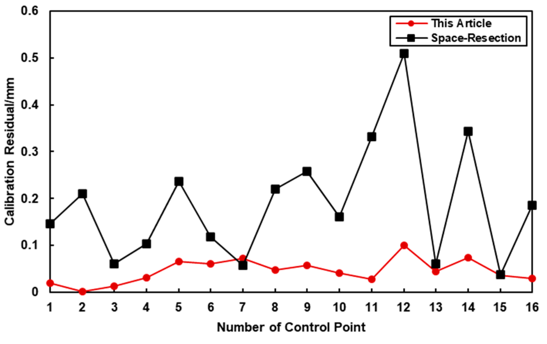
4.2. Calibration Progress of the Relationship between the Transmitter and Turntable

To verify the calibration accuracy of the proposed calibration method, the traditional space-resection method was applied to calibrate the relationship between the turntable and the transmitter, and the residuals of the target function were used to evaluate the calibration accuracy.
The setup for the calibration of the relationship between the transmitter and turntable is shown in Figure 12. The ERP needed to be constructed first. There were 16 control points, with magnetic nests placed around the space. The volume of the experiment space was 10 × 6 × 3 m 3 , and a laser tracker measured the ERP at three different positions. The coordinates of the control points were calculated using a bundle adjustment algorithm [20].
After constructing the ERP, the first scanning angle of the first control point needed to be set to 180° by adjusting the turntable. The scanning angle of the transmitter changed because of the turntable’s rotation. When the scanning angle of the transmitter was close to 180°, the turntable’s movement depended on the difference between the target angle and the average value of the scanning angle after 300 measurements.
The calibration residual of the proposed method was calculated according to Equation (19), which was derived from Equation (15):
F = i = 1 2 ( [ a i b i c i d i ] [ R r t T r t 0 1 ] [ cos ( α ) sin ( α ) 0 0 sin ( α ) cos ( α ) 0 0 0 0 1 0 0 0 0 1 ] [ R c r T c r 0 1 ] [ x y z 1 ] ) 2
In this equation, F is the calibration residual of the control point; a i ,   b i ,   c i ,   d i is the plane parameter of the i th fanned laser; and R c r and   T c r are the rotation and translation matrices from the ERP coordinate system to the turntable coordinate system, respectively. R r t and   T r t are the rotation and translation matrices from the turntable coordinate system to the transmitter coordinate system, respectively.
The calibration residual of the space-resection method can be defined by Equation (20):
F = i = 1 2 ( [ a i b i c i d i ] [ cos ( θ i ) sin ( θ i ) 0 0 sin ( θ i ) cos ( θ i ) 0 0 0 0 1 0 0 0 0 1 ] [ R T 0 1 ] [ x y z 1 ] ) 2
In this equation, F is the calibration residual of the control point, a i ,   b i ,   c i ,   d i is the plane parameter of the i th fanned laser, R , T represent the extrinsic parameters, and θ i is the corresponding scanning angle.
The physical meanings of the calibration residuals in Equations (19) and (20) was similar, representing the distance from the control point to the measurement vector formed by the two fanned lasers. Thus, the residual was able to indicate the performance of calibration.
As shown in Figure 13, the average calibration function’s residual of the proposed method was lower than 0.04, whereas the calibration function’s residual of the traditional space-resection method was approximately 0.18. The results were higher than the simulations and analysis because of the decentralization between transmitter’s receivers and laser tracker’s reflectors.

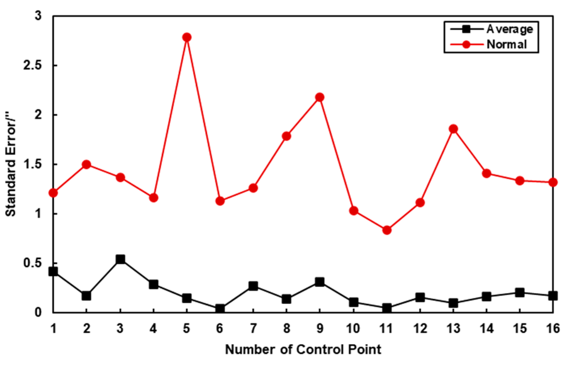
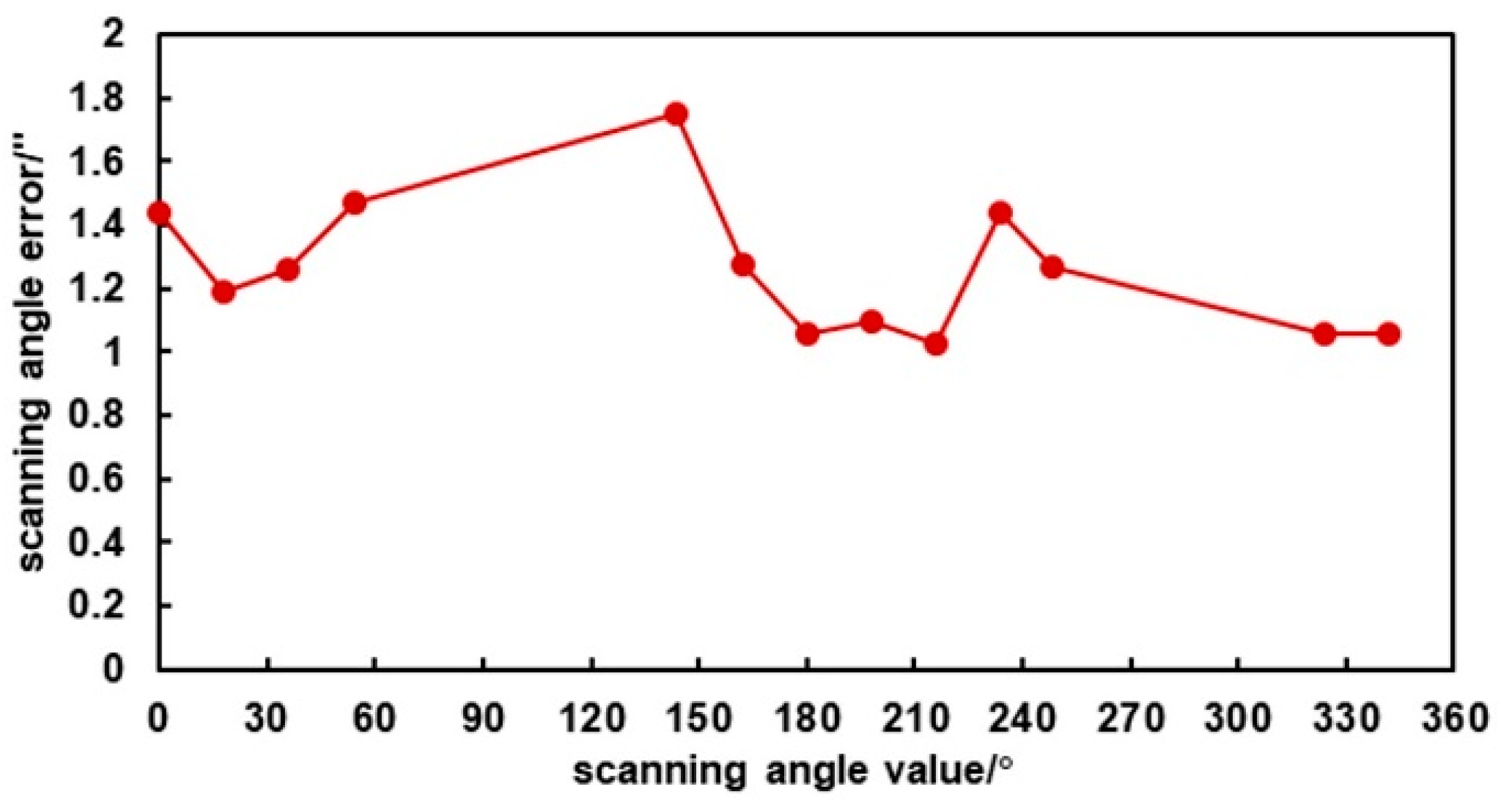
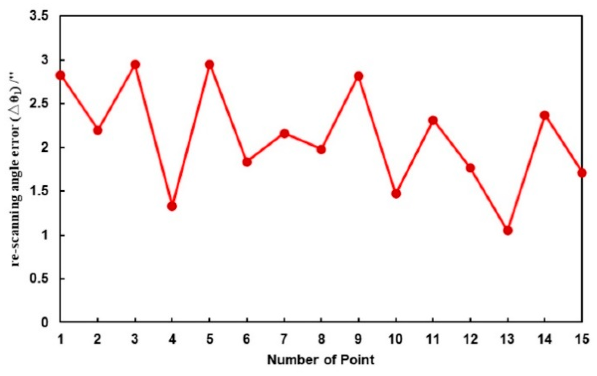
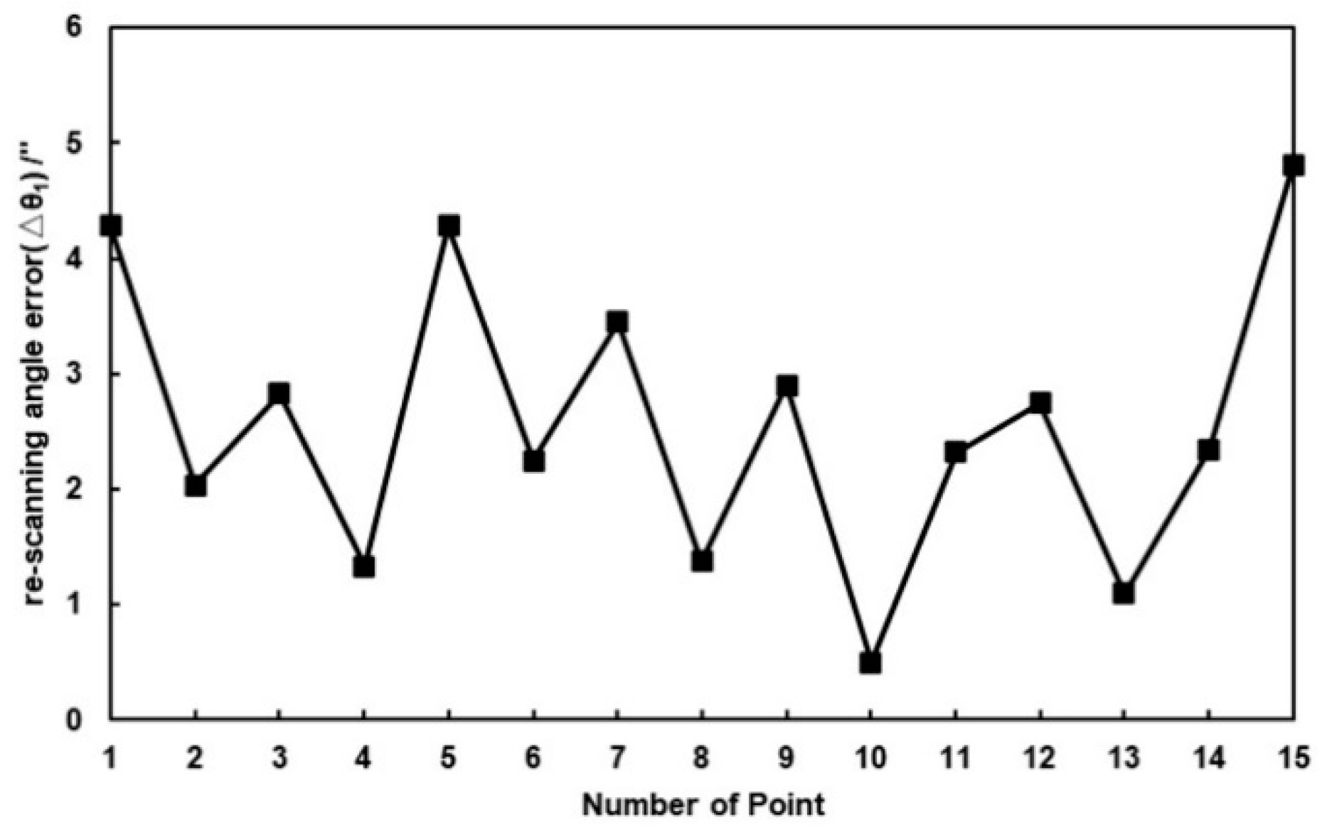
4.3. Evaluation of Scanning Angle Error in Different Positions

The evaluation was applied with the calibrated rotation and translation matrix from the turntable to the transmitter. The experimental setup is shown in Figure 11, and the process is illustrated in Figure 9. The turntable was used to provide the equivalent scanning angle results combined with the repeatability of the transmitter to substitute the scanning angle measured by the transmitter directly.
As shown in Figure 14, 13 scanning angles were chosen to test the transmitter’s scanning angle measurement error. The turntable’s reference angle and the transmitter’s scanning angle were obtained for each point. The difference between the aforementioned angle and the virtual scanning angle was determined. The transmitter’s scanning angle was recorded as the scanning angle measurement error of the wMPS transmitter.
The results in Figure 15 show that the maximum angle measurement error was approximately 2.79 arc seconds, and the average angle measurement error was approximately 1.26 arc seconds.
The uncertainty regarding the scanning angle was calculated by assuming that the uncertainty in the first and second scanning angles was equal. According to the uncertainty calculation, Equation (21), the uncertainty of the angle measurement result was approximately 1.7 arc seconds, with k = 1.
U θ 1 = U Δ θ 2 + U θ r e f 2
Furthermore, the results show that the angle measurement error was uniform. An inconsistency of the errors at various points could be attributed to the receiver’s orientation, leading to a decentralization error between the transmitter’s receiver and the laser tracker’s reflector.

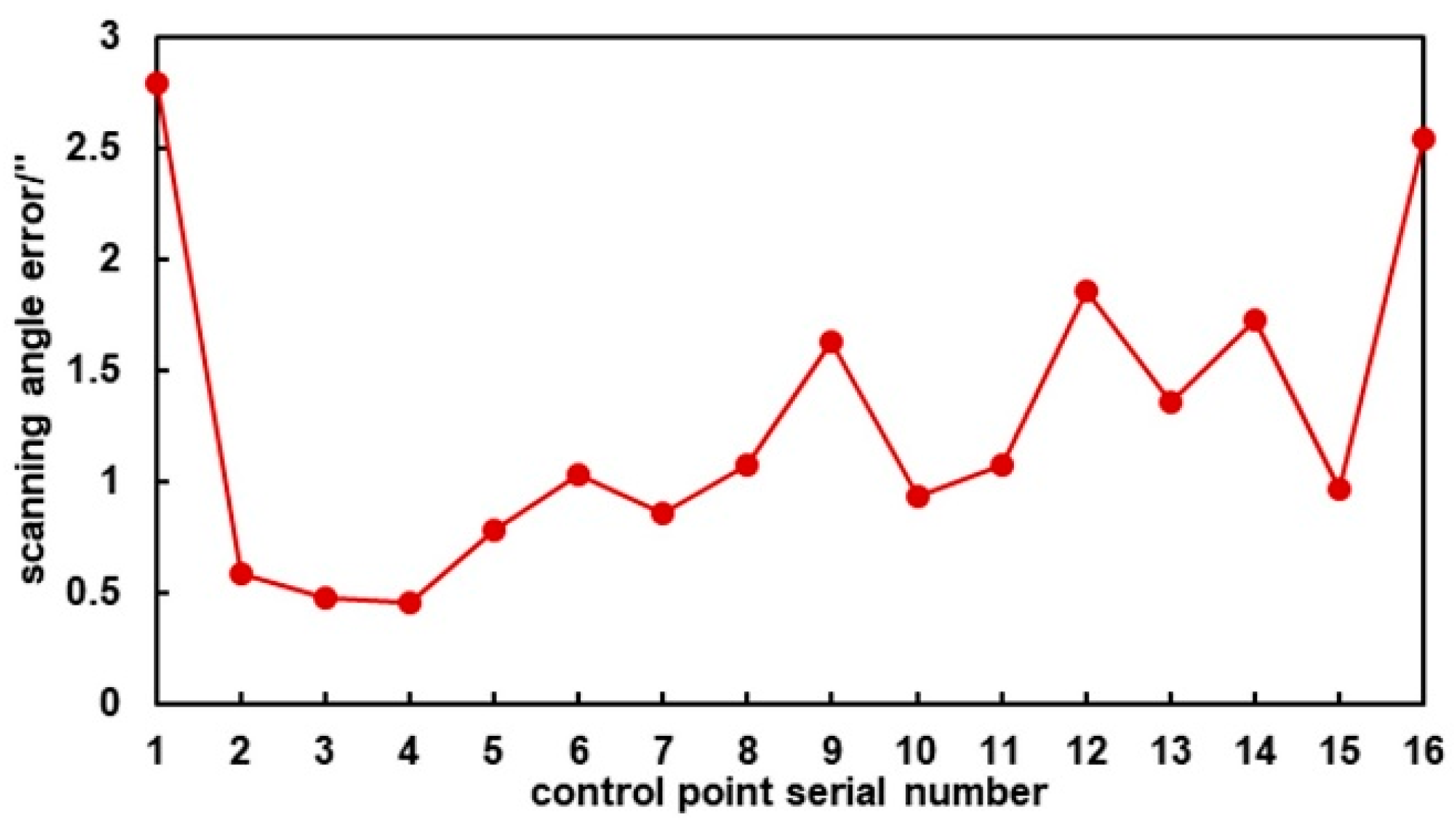
4.4. Verification by Coordinate Measurement

Since wMPS is a coordinate measuring machine, it was necessary to carry out a multi-transmitter intersecting measurement experiment to verify the effect of scanning angle measurement on coordinate measurement results. The coordinate measurements results were compared with the laser tracker Leica AT960, and the coordinate measurement error was converted into a scanning angle error and demonstrated.
To eliminate other errors, only one transmitter was selected to finish the coordinate measurement accuracy evaluation by multi-position measurement. After the extrinsic parameters and model parameters of the transmitters were calibrated, the 3-D coordinates of receivers could be calculated by Equation (5).
In the measurement volume, twelve receivers were selected to verify the coordinate measurement accuracy. Moreover, the coordinates were measured by a laser tracker, which had better accuracy than wMPS. These were considered as the ground-truth values. To evaluate the coordinate measurement error in terms of the re-scanning angle θ 1 , the re-scanning angle was defined as Equation (22):
θ 1 = arg min ( [ a 1 b 1 c 1 ] ( [ R 1 R 2 R 3 R 4 R 5 R 6 R 7 R 8 R 9 ] [ X Y Z ] + [ T X T Y T Z ] ) + d 1 ) 2
In this equation, a 1 , b 1 , c 1 is the normal vector of the first fanned laser; R and T are the extrinsic parameters; and X , Y , Z is the coordinate of the test point under the laser tracker’s coordinate system.
The re-scanning angle error Δ θ 1 was defined as Equation (23):
Δ θ 1 = θ 1 θ 1
θ 1 is the scanning angle derived by direct measurement, and θ 1 is the re-scanning angle calculated by Equation (21).
As shown in Figure 16, the average re-scanning error was 2.17 arc seconds, which is considerable to that obtained in Section 4.3, and the standard error was 0.58 arc seconds. The calibration process and data fusion process of each system may have introduced extra errors.
As shown in Figure 17, the average re-scanning error was 2.57 arc seconds, and the standard error was 1.20 arc seconds, which is higher. This result indicates that the horizontal- and vertical-angle-based angle measurement evaluation method is highly influenced by the EPR arrangement due to the fanned lasers and shaft assembly errors.

5. Conclusions

This study proposed a turntable-based evaluation method for the wMPS transmitter to evaluate the scanning angle. The measurement model based on the scanning angle was discussed, and was not affected by assembly errors. The method also included a calibration method for the relationship between the turntable and the wMPS transmitter. To ensure calibration accuracy, an estimation of the repeatability of the wMPS transmitter was applied to test the transmitter’s performance. Moreover, the mathematical model of the proposed method was also discussed. A Monte Carlo simulation was utilized to verify the calibration accuracy of the proposed calibration method. Furthermore, the calibration method was compared with the traditional space-resection method in a 10 × 6 × 3 m 3 space.
The experimental results show that the average calibration residual of the proposed method is lower than 0.04, whereas that of the traditional calibration method is approximately 0.18. The results demonstrate that the proposed calibration method has higher accuracy, and satisfies the evaluation of the angle measurement error.
Finally, this study compared the virtual scanning angle calculated by the turntable’s reference with actual scanning angles. The results show that the uncertainty of the angle measurement results is approximately 1.7 arc seconds with k = 1.

Author Contributions

Conceptualization, R.Z. and J.L.; methodology, R.Z.; software, R.Z.; validation, R.Z. and K.S.; writing—original draft preparation, R.Z.; writing—review and editing, S.S. and J.L.; project administration, J.Z. All authors have read and agreed to the published version of the manuscript.

Funding

This work was supported by the National Natural Science Foundation of China (Grant 51835007, Grant 52127810 and Grant 52205572).

Institutional Review Board Statement

Not applicable.

Informed Consent Statement

Not applicable.

Data Availability Statement

The data that support the findings of this study are available upon reasonable request from the authors.

Conflicts of Interest

The authors declare no conflict of interest.

References

  1. Fan, K.-C.; Chen, L.-C. Special Issue on Precision Dimensional Measurements. Appl. Sci. 2019, 9, 3314. [Google Scholar] [CrossRef]
  2. Schmitt, R.H.; Peterek, M.; Morse, E.; Knapp, W.; Galetto, M.; Hartig, F.; Goch, G.; Hughes, B.; Forbes, A.; Estler, W.T. Advances in Large-Scale Metrology—Review and future trends. CIRP Ann. 2016, 65, 643–665. [Google Scholar] [CrossRef]
  3. Franceschini, F.; Galetto, M.; Maisano, D.; Mastrogiacomo, L. Large-scale dimensional metrology (LSDM): From tapes and theodolites to multi-sensor systems. Int. J. Precis. Eng. Manuf. 2014, 15, 1739–1758. [Google Scholar]
  4. Franceschini, F.; Galetto, M.; Maisano, D.; Mastrogiacomo, L.; Pralio, B. Distributed Large-Scale Dimensional Metrology: New Insights; Springer Science & Business Media: Berlin/Heidelberg, Germany, 2011. [Google Scholar]
  5. Hao, Q.; Zhang, Y.; Fan, S.; Jiang, P.; Yin, H.; Xu, D. A novel three-dimensional coordinate positioning algorithm based on factor graph. IEEE Access 2020, 8, 207167–207180. [Google Scholar]
  6. Maisano, D.A.; Mastrogiacomo, L. Determining the extrinsic parameters of a network of large-volume metrology sensors of different types. Precis. Eng. 2022, 74, 316–333. [Google Scholar] [CrossRef]
  7. Muelaner, J.E.; Wang, Z.; Jamshidi, I.; Maropoulos, P.G.; Mileham, A.R.; Hughes, E.B.; Forbes, A.B. Study of the uncertainty of angle measurement for a rotary-laser automatic theodolite (R-LAT). Proc. Inst. Mech. Eng. Part B J. Eng. Manuf. 2009, 223, 217–229. [Google Scholar] [CrossRef]
  8. Zhao, J.; Ren, Y.; Lin, J.; Yin, S.; Zhu, J. Study on verifying the angle measurement performance of the rotary-laser system. Opt. Eng. 2018, 57, 044106. [Google Scholar] [CrossRef]
  9. Qiang, H.; Hongliang, Y.; Dingjie, X.; Bo, Z. Research on the IGPS device error and its influence of positioning accuracy. In Proceedings of the 2017 Forum on Cooperative Positioning and Service (CPGPS), Harbin, China, 19–21 May 2017; pp. 294–299. [Google Scholar]
  10. Muelaner, J.E.; Wang, Z.; Martin, O.; Jamshidi, J.; Maropoulos, P.G. Verification of the indoor GPS system, by comparison with calibrated coordinates and by angular reference. J. Intell. Manuf. 2012, 23, 2323–2331. [Google Scholar] [CrossRef]
  11. Schmitt, R.; Nisch, S.; Schnberg, A.; Demeester, F.; Renders, S. Performance evaluation of iGPS for industrial applications. In Proceedings of the 2010 International Conference on Indoor Positioning and Indoor Navigation, Zurich, Switzerland, 15–17 September 2010. [Google Scholar]
  12. Su, W.; Guo, J.; Liu, Z.; Jia, K. An intrinsic parameter calibration method for R-LAT system based on CMM. Int. J. Adv. Manuf. Technol. 2022, 120, 3155–3165. [Google Scholar] [CrossRef]
  13. American National Standards Institute. Performance Evaluation of Laser-Based Spherical Coordinate Measurement Systems; American Society of Mechanical Engineers: New York, NY, USA, 2006. [Google Scholar]
  14. Hughes, B.; Forbes, A.; Lewis, A.; Sun, W.; Veal, D.; Nasr, K. Laser tracker error determination using a network measurement. Meas. Sci. Technol. 2011, 22, 045103. [Google Scholar] [CrossRef]
  15. Icasio-Hernández, O.; Bellelli, D.A.; Vieira, L.H.B.; Cano, D.; Muralikrishnan, B. Validation of the network method for evaluating uncertainty and improvement of geometry error parameters of a laser tracker. Precis. Eng. 2021, 72, 664–679. [Google Scholar] [CrossRef] [PubMed]
  16. Wang, L.; Muralikrishnan, B.; Hernandez, O.I.; Shakarji, C.; Sawyer, D. Performance evaluation of laser trackers using the network method. Measurement 2020, 165, 108165. [Google Scholar] [CrossRef]
  17. Predmore, C.R. Bundle adjustment of multi-position measurements using the Mahalanobis distance. Precis. Eng. 2010, 34, 113–123. [Google Scholar] [CrossRef]
  18. More, J.J. The Levenberg-Marquardt algorithm: Implementation and theory. Lect. Notes Math. 1978, 630, 105–116. [Google Scholar]
  19. Lin, J.R.; Sun, J.L.; Yang, L.H.; Zhang, R.; Ren, Y.J. Modeling and Optimization of Rotary Laser Surface for Large-Scale Optoelectronic Measurement System. IEEE Trans. Instrum. Meas. 2021, 70, 1–9. [Google Scholar] [CrossRef]
  20. Xiong, C.; Bai, H. Calibration of Large-Scale Spatial Positioning Systems Based on Photoelectric Scanning Angle Measurements and Spatial Resection in Conjunction with an External Receiver Array. Appl. Sci. 2020, 10, 925. [Google Scholar] [CrossRef]
Figure 1. (a) Traditional measurement model; (b) assembly errors of laser devices and shafts.
Photonics 10 01224 g001
Figure 2. The time difference generated by fanned-laser rotation.
Photonics 10 01224 g002
Figure 3. Definition of the scanning angle.
Photonics 10 01224 g003
Figure 4. Measurement principle of wMPS.
Photonics 10 01224 g004
Figure 5. Simulation results regarding the effects of fanned lasers and shaft assembly errors on the horizontal angle.
Photonics 10 01224 g005
Figure 6. Simulation results regarding the effects of fanned lasers and shaft assembly errors on the vertical angle.
Photonics 10 01224 g006
Figure 7. Calibration setup for the proposed method.
Photonics 10 01224 g007
Figure 8. The schematic of turntable adjustment.
Photonics 10 01224 g008
Figure 9. Experimental process.
Photonics 10 01224 g009
Figure 10. Monte Carlo simulation results for the space-resection calibration method and the proposed method.
Photonics 10 01224 g010
Figure 11. Results of repeatability of wMPS transmitter.
Photonics 10 01224 g011
Figure 12. Setup for the calibration of the relationship between the transmitter and the turntable.
Photonics 10 01224 g012
Figure 13. Comparison of calibration residual for the proposed calibration method and the space-resection method.
Photonics 10 01224 g013
Figure 14. The scanning angle error evaluated by the proposed method (the x-axis represents the scanning angle of the transmitter).
Photonics 10 01224 g014
Figure 15. The scanning angle error evaluated by the proposed method (the x-axis represents the point serial number).
Photonics 10 01224 g015
Figure 16. The re-scanning angle errors.
Photonics 10 01224 g016
Figure 17. The re-scanning angle errors, based on horizontal and vertical angles.
Photonics 10 01224 g017
Disclaimer/Publisher’s Note: The statements, opinions and data contained in all publications are solely those of the individual author(s) and contributor(s) and not of MDPI and/or the editor(s). MDPI and/or the editor(s) disclaim responsibility for any injury to people or property resulting from any ideas, methods, instructions or products referred to in the content.

