Article

Single-Shot, Pixel-Encoded Strip Patterns for High-Resolution 3D Measurement

1
College of Intelligent Systems, Science and Engineering, Harbin Engineering University, Harbin 150001, China
2
Department of Information and Communication System, Harbin 150001, China
*
Authors to whom correspondence should be addressed.
Photonics 2023, 10(11), 1212; https://doi.org/10.3390/photonics10111212
Submission received: 19 September 2023 / Revised: 27 October 2023 / Accepted: 28 October 2023 / Published: 31 October 2023
(This article belongs to the Special Issue Advances and Application of Structured Light)

Abstract

:
In this research, we combined two distinct, structured light methods, the single-shot pseudo-random sequence-based approach and the time-multiplexing stripe indexing method. As a result, the measurement resolution of the single-shot, spatially encoded, pseudo-random sequence-based method improved significantly. Since the time-multiplexed stripe-indexed-based techniques have a higher measurement resolution, we used varying stripes to enhance the measurement resolution of the pseudo-random sequence-based approaches. We suggested a multi-resolution 3D measurement system that consisted of horizontal and vertical stripes with pixel sizes ranging from 8 × 8 to 16 × 16. We used robust pseudo-random sequences (M-arrays) to controllably distribute various stripes in a pattern. Since single-shape primitive characters only contribute one feature point to the projection pattern, we used multiple stripes instead of single-shape primitive symbols. However, numerous stripes will contribute multiple feature points. The single character-based design transforms into an increased featured size pattern when several stripes are employed. Hence, the projection pattern contains a much higher number of feature points. So, we obtained a high-resolution measurement. Each stripe in the captured image is located using adaptive grid adjustment and stripe indexing techniques. The triangulation principle is used to measure 3D.

1. Introduction

Structured light (SL) techniques are used in many 3D object-sensing applications, such as mobile devices [1], medical imaging [2], intelligent welding robots [3], high-temperature object detection [4], industrial quality inspection [5,6], and finding defects in manufacturing and packaging [7]. Various SL techniques have evolved in the past few decades [8,9], wavering from time-multiplexing or sequential to real-time single-shot 3D measurement [10]. SL methods are classified into spatial neighborhood and temporal coding schemes [11]. The SL can provide high measurement accuracy and dense 3D information. However, the SL methods are more sensitive to surface color and texture. Many commercial devices, such as Microsoft RGB-D, Microsoft Kinect v1, Intel RealSense D435, and Orbbec Astra Pro cameras, map depth through speckle-based projections [12]. However, their depth resolution and accuracy are lower. In contrast, we suggest a multi-resolution method based on various stripes with good resolution and accuracy.

1.1. Related Work

Our approach integrated two strategies, i.e., stripe indexing-based techniques previously employed as time-multiplexed patterns that converge into a single shot and 2D spatial neighborhood, using pseudo-random sequence (M-arrays)-based methods. This section will cover the significant developments in both of these strategies.
The time multiplexing techniques include methods based on binary coding, gray coding, phase shift, photometric, and hybrid techniques that led researchers toward developing fringe patterns. The methods based on fringe patterns have the limitations of lower accuracy and resolution and require sequential projections [13,14]. Nguyen et al. [15] proposed 16 frames of fringe patterns to train CNN. When combined with speckle projection, the fringe pattern can provide single-shot measurement [16]. However, the image acquisition and processing time are high since phase unwrapping is required. In contrast to the fringe patterns, the suggested approach is spatially encoded, single-shot, and employed for real-time applications.
The strip-indexed-based methods are time multiplexing, requiring several frames to project. However, they are employed for high-resolution measurements. For example, ‘m’ stripe patterns can encode 2m stripes [17], a line-shifting technique applies 32 projections [18], and the N-ary reflected gray code uses multiple gray levels for pattern illumination [19]. Multiple gray-level stripes encode a pattern with fewer projections [20].
The 3D measurement techniques often use single-shot stripe-based patterns [21]. The examples are stripe patterns based on three gray levels [22], segmented stripes with random cuts [23], and a high-contrast color stripe pattern for fast-range sensing [24,25]. These single-shot strip-based methods have a lower resolution. In contrast, we proposed a single-shot, pseudo-random sequence-based stripe pattern for high-resolution measurement.
The spatial projection techniques can differentiate into full-frame spatially varying color patterns, single-shot stripe indexing (1D grid), and 2D grid patterns [26]. The fast and real-time SL techniques are based on a spatially encoded grid and fringe patterns [27]. The main principle of spatial codification techniques is to ensure the distinctiveness of the codeword at any location in the pattern, and that location is determined from the surrounding points. Examples of the spatial neighborhood are the patterns based on non-formal coding [23,28], the De Bruijn sequence [29,30,31,32], pseudo-random sequences (PRSs) or M-arrays [2,33,34,35,36,37,38], and speckle projection techniques [39,40,41]. The spatial coding scheme has the advantage that 3D measurements can be achieved with a single projection and a single capture image.
The SL techniques based on the De Bruijn sequence employ colored stripe patterns [29] and dynamic programming [31], optimized De Bruijn [30], color slits [32], and shape primitive-based designs for single-shot measurements. However, De Bruijn patterns provide a relatively low density and resolution, and the number of color stripes restricts the precision of 3D reconstruction, and an interpolation operation is also necessary.
The pseudo-random sequence-based, or M-array methods can be divided into two types, i.e., colored encoded designs or monochromatic geometric symbol-based schemes.
The patterns are further distinguished into color-coded grid lines [42,43] and primitives such as dots/circles [34,44], rectangles [36,38,45,46,47], or diamond-shaped elements [48,49]. Since all these methods are based on multiple colors, they are immune to noise and segmentation errors due to highly saturated surface colors. They can easily warp through the intrinsic shades of the measuring surface.
A monochromatic geometric symbol-based approach is an alternative to color encoding schemes since the single-shot SL can encode through colors or geometrical features [50]. These methods are more robust to the effect of ambient light, uneven albedos, and colors in scenes [51]. The examples are those proposed by Albitar et al. [2,52], Yang et al. [53], Lu et al. [35], Tang et al. [54], Ahsan [33], and Zhou et al. [55] using pseudo-random sequences with a feature size of 27 × 29, 27 × 36, 48 × 52, 65 × 63, 45 × 72, and 98 × 98, respectively.
The researchers, who used pseudo-random sequences through either color or monochromatic geometric symbols, have tried to increase the measuring resolution by increasing the number of feature points. The primitives employed contributed only one feature point. In this research, we introduced stripes instead of single-centroid symbols, significantly increasing the number of feature points.
In the alternative approach of speckle projection, the accuracy relies heavily on the determined geometric parameters depicting the relationship between out-of-plane height and in-plane speckle motion, i.e., the measured surface in-plane displacements with respect to speckle motion. Much research has been proposed to overcome the limitations in speckle profilometry [39,40,41]. Speckle projection can provide dense reconstruction but with lower accuracy. In contrast, shaped–coded spatial SL can provide higher accuracy [56].
Our previous work [33] presented a multi-resolution system that can generate robust pseudo-random sequences of any desired size required to encode with projector resolution. The projection pattern encodes digitally through pixels that can adopt any projector and resolution. For example, the digital forms of spatial light modulators (SLMs) are used in optics for super-resolution. Since they can provide the smallest pixels and the largest field of view (FOV) [57], they can provide fine-grained light control, creating two-dimensional patterns with user-controllable characteristics that consist of arrays of pixels [58]. Each pixel of SLM can be controlled individually by the phase or amplitude of light passing through it or reflecting off it [59]. These devices can act as super-controllable microscale projectors. The suggested method also provides flexibility in measurement resolution while choosing a projector. The proposed approach and our previous work can be used to implement SL designs in SLMs and other projector devices. One can choose its measurement resolution; with that choice, the projection pattern can be designed according to the required projector size and resolution.

1.2. Major Contribution of This Paper

We proposed a flexible method to design patterns according to surface area requirements and measuring resolution. The significant contributions of this article are as follows:
(1)
We combined two approaches proposed by various researchers, i.e., the high-resolution, time multiplexing stripe indexing method with the comparatively low resolution, single-shot, spatially encoded pseudo-random-sequence method to improve its measurement resolution.
(2)
Using the multi-resolution system, we proposed pixel-defined, digitally encoded stripe patterns for high-resolution, single-shot 3D measurements.
(3)
We computed the proposed method’s percentage increase in feature points, which benefits in increasing the measurement resolution. The results show significant improvements in measuring resolution.
(4)
A new strategy for decoding captured image patterns is explained, using stripe indexing and adaptive grid adjustment.

2. Materials and Methods

2.1. Designing of Pattern

This section will explain the process of forming a strip-based projection pattern using a pseudo-random sequence.

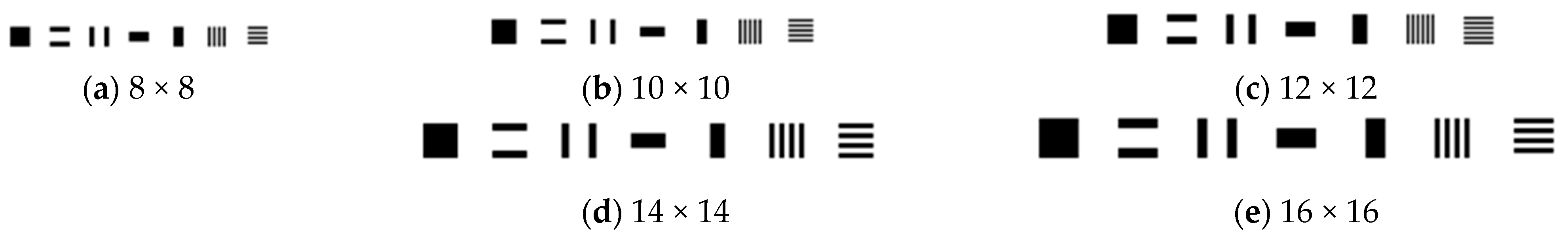
2.1.1. Defining Various Stripe Types

Stripes are natural carriers of direction or orientation information and are easy to decode using the area functions. Previously, small stripe patterns were used to eliminate inter-reflections in 3D reconstruction [60]. So, we proposed a design using various small stripes. We proposed a multi-resolution system in which stripe sizes vary from 8 × 8 to 16 × 16 pixels in symbol space. The stripes form the projection pattern depicted in Figure 1. The square-shaped stripe at the number 1 position in Figure 1 uses the maximum area in the pixel space. Similarly, horizontal and vertical stripes at numbers 4 and 5 are placed in Figure 1, which has precisely 1/2 (half) the size of the maximum area in the pixel space. Likewise, the pairs of horizontal and vertical stripes parallel to each other at the number 2 and 3 positions are 1/4 (quarter) of the size of the maximum area in the pixel space. Similarly, the four horizontal and four vertical stripes parallel to each other at number 6 and 7 positions in Figure 1 use precisely 1/8th (one eight) of the size of the maximum area in the pixel space. The other significant properties of these stripes are their aspect ratios, orientation, eccentricity, and equivalent diameter. These properties will be used at the decoding stage of the pattern. We will define and calculate each of these properties in the decoding section.

2.1.2. Pseudo-Random Sequences or (M-Arrays)

To spread these stripes in a projection pattern in a controllable manner, we generated M-arrays of various sizes to use with varying stripe sizes from 8 × 8 to 16 × 16. We formed the M-arrays using the method described in [33]. We used a projector with a resolution of 800 × 1280 and proposed a multi-resolution system with patterns employing five sets of stripes. We generated five M-arrays corresponding to each pixel size. Each M-array consisted of seven alphanumeric bases corresponding to seven stripe types. The robustness of the codewords in all M-arrays was ensured by computing the Hamming distances between each codeword. The dimensions, the number of alphabets, Hamming distances, and the percentile of the robust codewords are shown in Table 1. The Hamming distance profiles of each M-array formed for use in the projection pattern are illustrated in Figure 2. The profiles of M-arrays reflected that most of the codewords have a Hamming distance greater than three. About 70% of codewords have the Hamming distances of 8 and 9. About 97% of the codewords have Hamming distances of 6 and higher, and 99% have Hamming distances of 5 and higher, proving that the generated M-arrays are highly robust.

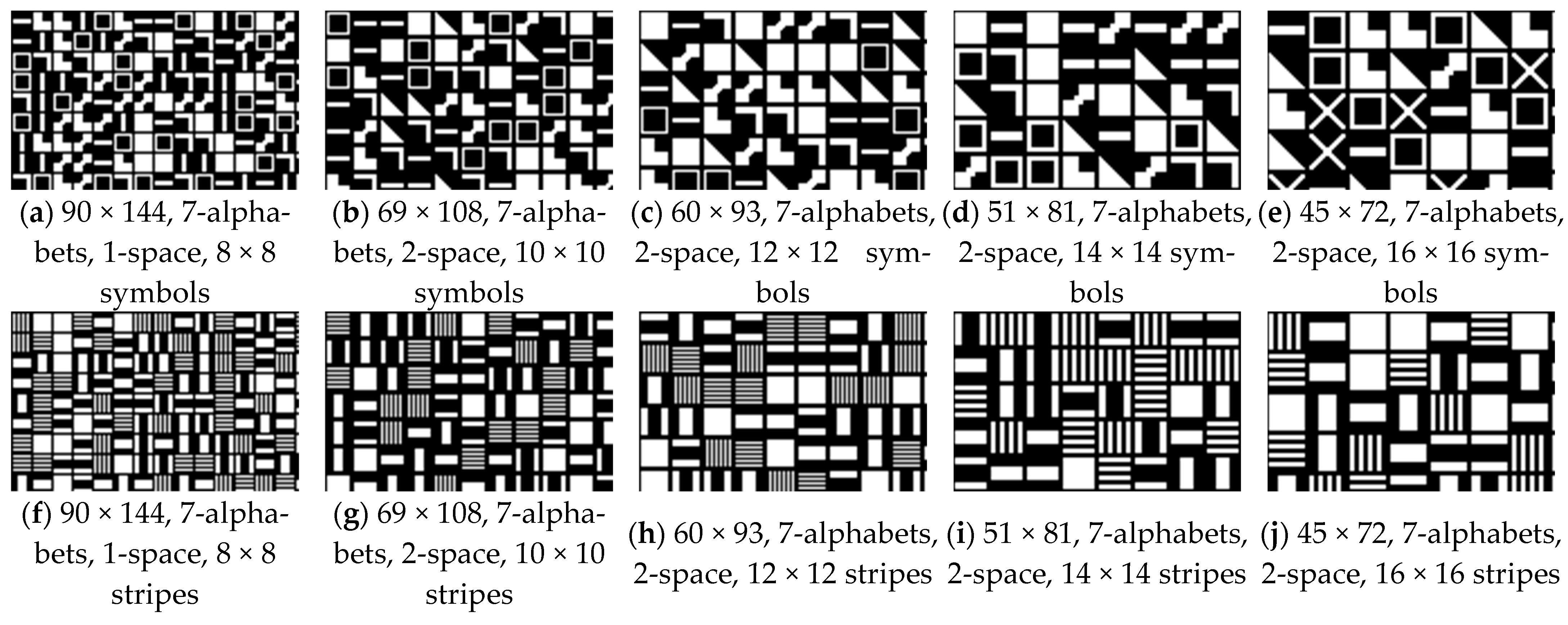
2.1.3. Formation of Projection Pattern

We used five M-arrays with seven alphabets to generate five projection patterns using single-centroid symbols, just like in [33], and five projection patterns using the stripes-based approach that we suggest in this paper. The parts of five generated projection patterns using single-centroid alphabets and stripe-based designs are shown in Figure 3.

2.1.4. Computation and Comparison of Feature Points

We compared the feature points in two designs, which improved measured resolutions in the proposed pattern. As described in our previous work [34], the generated M-arrays are slightly larger than the required dimension of projectors and round to the multiple of 3. The feature points in the projection pattern are not simply the number of elements obtained by multiplying the dimensions of an M-array. The feature points in the complete projection pattern while using single-centroid-based symbols can be calculated with the help of the following relationship:
X F P = R l o w ( X P P S r e s + S S p a c e )
Y F P = R l o w ( Y P P S r e s + S S p a c e )
F P = X F P × Y F P
where XFP and YFP are the X and Y dimensions of feature points in the projection pattern. Rlow is the round function to the lowest integer. XPP and YPP are the X and Y dimensions of projector resolution. Sres is the measuring resolution or stripe size employed in the projection pattern. Sspace is the pixel spacing between two adjacent alphabets in a projection pattern. FP is the number of feature points in the projection pattern.
The feature points in stripe-based patterns can be computed through computer programming since different stripes are randomly distributed in the projection pattern. The computation of the number of feature points in a single-centroid symbol-based design, strip-based approach, and a percentage increase in feature points in the strip-based method is depicted in Table 2. We defined a new parameter ‘α’ as the ratio of increase in feature points in a stripe-based approach to a single centroid-based symbol pattern. It is worth noting that the 3D measuring resolution will improve with the same ratio as the increase in feature points.
The bar graph shows the increase in feature points of the projection pattern while using the stripe pattern, depicted in Figure 4. As evident from Table 2 and the bar graph in Figure 4, the feature points are significantly increased almost twice in all types of measuring resolution of a pattern from 8 × 8 pixels to 16 × 16 pixels while using the same M-arrays to create projection patterns. Using stripe-based designs for increasing measuring resolution will have a significant advantage.

2.2. Decoding of Pattern

Currently, many researchers have used deep learning to decode structured light patterns, such as CNN [15], the learning-based approach [61], dual-path hybrid network UNet [62], fringe-to-fringe network [63], and MIMONet [64] to decode the phase information from the projected fringe pattern. All of these techniques solve fringe-pattern-based projections. The accumulation of these techniques to form a dataset is comparatively straightforward since DNNs learn from massive datasets with supervised labels. There are very few decodings of patterns using DNN learning techniques employing other SL approaches. One such dataset used CNN to decode eight geometrical-based symbols [65]. Since the implementation of deep-learning algorithms requires three essential elements: (1) large-scale 3D datasets, (2) obtainable structure and training, and (3) graphics processing units (GPU) for the acceleration of the system [66], all of these three factors are fundamental for the employment of deep-learning methods. The challenges of forming datasets and their training make them slow and complex processes for computation. In contrast, our decoding method employs area functions and shape description parameter ratios [67,68]. It is a simple process since it needs less computational power than deep learning. Therefore, the complexity of the algorithm and the hardware requirements are reduced, which is also a significant advantage.

2.2.1. Preprocessing, Segmentation, and Labelling

Preprocessing is the first step for decoding. The captured image is prepared for decoding in this step. The captured image from the measuring surface first undergoes image contrast enhancement and noise removal through filtering. A segmentation algorithm is applied to the captured image to obtain a binary image. The segmentation has a significant impact on the decoding process. The neighborhood stripes may merge if the segmentation process is more vigorous, and if it is weaker, many binary regions that can decoded as stripes may omitted. Hence, a balance is required. We obtained the best results using morphological Mexican top hat filtering and then applied the optimum global thresholding using Otsu methods [69]. After segmentation, labeling is carried out. The binary regions obtained through segmentation will be labeled with specific region numbers using the algorithm specified by Haralick [70].

2.2.2. Computation of Parameters

To decode and classify the stripes used in the pattern, we used area functions and shape description parameters, such as aspect ratio, eccentricity, orientation, parameter-to-area ratio, circularity ratio, and orientation. These shape descriptor parameter-based classifications are stable against sensor noise, illumination changes, and color variation. Most shape descriptors are computed through regional moments [71,72]. The essential shape description parameters used in the classification and decoding are defined in Table 3.
Table 4 shows the values of shape descriptive parameters for each stripe type. The threshold values computed in Table 4 are employed to decode and classify the stripes in a pattern. Three additional parameters, centroid x ¯ , y ¯ , orientation ( θ ), and grid distance (grid), are also computed. The location of each stripe is identified with the help of centroids, and orientation is used to find the direction. These additional parameters are used in searching the neighborhoods and establishing correspondences. Since stripes are natural carriers of direction information, each stripe in our pattern carries its orientation. Only the square-shaped strips may not have their direction, so this problem is resolved by attaining its angle from the nearest stripe. The vertical stripes’ orientation has an offset of 90 degrees, so their orientation will adjust accordingly in computation by subtracting 90 degrees from their orientation angle.

2.2.3. Classification of Stripes

The seven types of stripes used in these patterns are classified using the shape description parameters defined in Table 3, and their corresponding threshold values are calculated in Table 4. The shape description parameters like eccentricity, aspect ratio, parameter-to-area ratio, circularity ratio, area-function ratio, and orientation are used to classify the symbols. The classification parameters are optimized using the trial and error method. In the classification process, we selected the range of values for each parameter and recorded the results. The values lock where the maximum number of stripes classifies in each pattern. The deformation caused by the projector and camera due to the angle of incidence compensates by using a range of values for each parameter used in the classification. The errors in decoding are minimized if more shape description parameters differentiate stripes.
The various size stripes used in the pattern can be easily differentiable using area function ratios since each type of stripe is precisely proportionate to the area compared to the other types of stripes. For example, square-shaped stripes have the maximum extent of space, and all other stripes are proportional to their size. So, in the first level of abstraction, the area sizes are compared from the maximum level, and specific threshold values are set for each stripe type to obtain this abstraction. The eccentricity ratio is used for the second level of differentiation. The square-shaped stripes can easily differentiate from other stripes as they have eccentricity values near zero, while all other stripes have eccentricity values ranging from 0.75 to 1. Further classification is carried out through the aspect ratio (AR) since square-shaped stripes have an AR equal to one, and a single thick horizontal or vertical stripe has an AR of two. In contrast, two parallel horizontal and vertical stripes have an AR of four, and four parallel stripes have an AR nearly equal to eight. The circularity ratio (CR) is the next level of abstraction. The squared-shaped stripe has a CR near to one, while all other stripes have a lower circularity ratio, ranging from 0.1 to 0.8. The further distinguishes can be obtained through a parameter-to-area ratio (PAR) since square-shaped stripes have the lowest PAR. In contrast, four parallel stripes have the highest PAR, with the PAR for other stripes ranging from 0.2 to 0.8. The horizontal and vertical stripes of the same types differentiate through their orientation.

2.2.4. Searching in the Neighborhood

After the classification and calculation of the parameters of each decoded stripe in the pattern, the next step is searching each stripe’s neighborhood to establish a correspondence between the pattern initially projected and the pattern obtained from the measuring surface. This is the most significant part of the decoding process. Due to the use of multiple stripes instead of single centroid symbols, the complexity of the pattern increases manifold. The neighborhood searching includes finding the successive or consecutive stripes or sets of stripes if multiple stripes are present and their next stripes to find the codeword size of 3 × 3. Searching in the area includes finding and estimating the position of all window elements around the stripe for which computations must endure. Figure 5 illustrates the mechanism of searching in the neighborhood.

Stripe Indexing and Adaptive Grid Adjustments

When multiple stripes or a set of stripes occur, their centroid values are not directly used to find the following consecutive stripes; instead, they virtually adjust to the center of the symbol space, and that altered value is used for finding the neighborhood stripes in the window of 3 × 3. Changing the centroid positions to find the neighborhood stripe is called adaptive grid adjustment. The first essential step for adaptive grid adjustments is finding the stripe part or index number. The stripe part numbers or indexes are determined by scanning or searching perpendicular to the major axis of the stripe. Searching or scanning is performed along the Y-axis and vice versa if the major axis is along the X-axis. Therefore, for stripe types 2 and 7, the major axis is parallel to the X-axis, so searching or scanning is performed on the upper and downward sides of the stripe. Similarly, scanning or searching is performed from left to right for stripe types 3 and 6, since the central axis is parallel to the Y-axis. The computation will include that angle effect if the stripe has some orientation.

Stripe Indexing for Stripe Types 2 and 3

The stripe types 2 and 3 always occur in pairs or groups of two parts, apart by approximately 0.8 times the grid distance. Scanning and computation of the Euclidian distance between consecutive stripes significantly influence finding their part or index number. The scanning or searching of the region performs at 0.9 times the grid to determine their part number. For stripe type 2 and type 3, whose central axis is along the X-axis and Y-axis, respectively, the scanning or searching executes for 0.9 times the grid. If a similar kind of stripe has occurred before the stripe, then its distance from the current stripe is computed. If the calculated distance is less than 0.5 times the grid distance, then the present stripe is marked as part 1; if the calculated distance is more than 0.5 times the grid distance, then the existing stripe index is marked as part 2. This procedure is shown in Figure 6.
The Euclidean distance between consecutive stripes is calculated by using the following relation:
D i s t a n c e consecutive stripes = x C S x P r e v 2 + y C S y P r e v 2
where ( x C S , y C S ) is the centroid of a current stripe whose part number or indexing must be determined. ( x p r e v , y p r e v ) is the centroid of the neighborhood stripe. If the distance (of consecutive stripes) is less than half of the grid distance, the current stripe part number or the index is determined to be 1. Alternatively, if the distance (of successive stripes) exceeds half the grid distance, the current stripe part number or index is determined to be 2.

Adaptive Grid Adjustment for Stripe Types 2 and 3

After finding the stripe index or part number of stripe types 2 and 3, the stripe’s centroid positions virtually change for estimating the neighborhood stripes’ centroid positions. The centroid positions are approximately 37.5% of the grid distance apart from the central place of the stripe space. Part 1 is above or on the left side of the central location. Part 2 is at the lower or right side of the middle area of the stripe space. Hence, centroid positions for both stripes (part 1 or 2) virtually adjust accordingly. The following relationship represents the virtually adjusted centroid positions for part 1:
x a d j _ 2 _ 1 = x C S 1 + G A sin θ
y a d j _ 2 _ 1 = y C S 1 + G A cos θ
x a d j _ 3 _ 1 = x C S 1 + G A cos θ
y a d j _ 3 _ 1 = y C S 1 G A sin θ
where ( x a d j _ 2 _ 1 , y a d j _ 2 _ 1 ) and ( x a d j _ 3 _ 1 , y a d j _ 3 _ 1 ) is the adjusted centroid position of part 1 of stripe type 2 and type 3. ‘ θ ’ is the direction of the current stripes whose adjusted centroid is to be determined. GA is the grid adjustment factor, equal to 0.375 times the grid.
The centroid positions for part 2 of stripe types 2 and 3 also adjust with the following relationship:
x a d j _ 2 _ 2 = x C S 2 G A sin θ
y a d j _ 2 _ 2 = y C S 2 G A cos θ
x a d j _ 3 _ 2 = x C S 2 G A cos θ
y a d j _ 3 _ 2 = y C S 2 + G A sin θ
where ( x a d j _ 2 _ 2 , y a d j _ 2 _ 2 ) and ( x a d j _ 3 _ 2 , y a d j _ 3 _ 2 ) are the virtually adjusted centroid position of part 2 of stripe types 2 and 3.

Stripe Indexing for Stripe Types 6 and 7

Stripe types 6 and 7 always occur in pairs of four stripes, which are apart by approximately a 0.25 grid distance from each other. Since each stripe is equidistant from the other, calculating the distance between consecutive stripes cannot play any role in indexing or assigning part numbers to adjust grid or centroid positions virtually. Therefore, scanning is performed multiple times to find a different stripe type in the same line. When a different type of stripe occurs in the line of consecutive stripes of stripe type 6 or 7, stripe indexing is performed by counting the stripe number from that other type to the existing stripe part number. The stripe counting is performed in the modulo of four stripes, i.e., the stripe part number or index repeats after every four stripes. If a different type of stripe is found at the beginning of stripe counting, then the procedure for stripe counting is executed by forward stripe counting to find the index of the current stripe. Similarly, if a different type of stripe occurs at the end of stripe counting, backward stripe counting is performed to find the stripe index of the current stripe. This method is shown in Figure 7.

Adaptive Grid Adjustment for Stripe Types 6 and 7

After finding the stripe index or part number of stripe types 6 and 7, the stripe’s centroid positions change virtually for estimating the neighborhood stripes’ centroid positions. Every stripe centroid position will adjust to the central space. For index numbers 1 and 4, the centroid positions are 40% of the grid distance apart from the central place of the stripe space. Part 1 is above or on the left side of the central location. Part 4 is the lower or right side of the central area of the stripe space. Hence, the stripes’ centroid positions (parts 1 and 4) adjust virtually. The following relationship represents the virtually adjusted centroid positions for part 1:
x a d j _ 7 _ 1 = x C S 1 + G A 1 sin θ
y a d j _ 7 _ 1 = y C S 1 + G A 1 cos θ
x a d j _ 6 _ 1 = x C S 1 + G A 1 cos θ
y a d j _ 6 _ 1 = y C S 1 G A 1 sin θ
where ( x a d j _ 7 _ 1 , y a d j _ 7 _ 1 ) and ( x a d j _ 6 _ 1 , y a d j _ 6 _ 1 ) are the adjusted centroid position of part 1 of stripe type 7 and type 6. GA1 is the grid adjustment factor, equal to 0.4 times the grid.
The centroid positions for part 4 of stripe types 7 and 6 also adjust virtually with the following relationship:
x a d j _ 7 _ 4 = x C S 4 G A 1 sin θ
y a d j _ 7 _ 4 = y C S 4 G A 1 cos θ
x a d j _ 6 _ 4 = x C S 4 G A 1 cos θ
y a d j _ 6 _ 4 = y C S 4 + G A 1 sin θ
where ( x a d j _ 7 _ 4 , y a d j _ 7 _ 4 ) and ( x a d j _ 6 _ 4 , y a d j _ 6 _ 4 ) are the adjusted centroid position of part 4 of stripe type 7 and type 6.
For index numbers 2 and 3, the centroid positions are 20% of the grid distance apart from the central place of the stripe space. Part 2 is above or on the left side of the central location. Part 3 is the lower or right side of the central area of the stripe space. So, the stripes’ centroid positions (parts 2 and 3) adjust virtually. The following relationship represents the virtually adjusted centroid positions for part 2:
x a d j _ 7 _ 2 = x C S 2 + G A 2 sin θ
y a d j _ 7 _ 2 = y C S 2 + G A 2 cos θ
x a d j _ 6 _ 2 = x C S 2 + G A 2 cos θ
y a d j _ 6 _ 2 = y C S 2 G A 2 sin θ
where ( x a d j _ 7 _ 2 , y a d j _ 7 _ 2 ) and ( x a d j _ 6 _ 2 , y a d j _ 6 _ 2 ) are the adjusted centroid position of part 2 of stripe type 7 and type 6. GA2 is the grid adjustment factor, equal to 0.2 times the grid.
The centroid positions for part 3 of stripe types 7 and 6 also virtually adjust with the following relationship:
x a d j _ 7 _ 3 = x C S 3 G A 2 sin θ
y a d j _ 7 _ 3 = y C S 3 G A 2 cos θ
x a d j _ 6 _ 3 = x C S 3 G A 2 cos θ
y a d j _ 6 _ 3 = y C S 3 + G A 2 sin θ
where ( x a d j _ 7 _ 3 , y a d j _ 7 _ 3 ) and ( x a d j _ 6 _ 3 , y a d j _ 6 _ 3 ) are the virtually adjusted centroid positions of part 3 of stripe type 7 and type 6.

Finding the Neighborhood Stripes

After finding the stripe index and the grid adjustment, the next step is to find the other elements of the neighborhood to compute the codeword of 3 × 3 for establishing the correspondence. The adjusted centroid positions are used to search the nearby neighborhood stripes. If the stripes are single stripes just as square-shaped (stripe number 1) or single horizontal (stripe number 4) or vertical stripes (stripe number 5), which lie at the center of the stripe space, then there is no need for indexing and grid adjustment. For these three types of stripes, their centroid positions are used to find or estimate the part of neighborhood stripes. The process of finding neighborhood stripes is shown in Figure 8.
So, the calculated centroid positions for the neighborhood stripes to scan or search along that location are obtained by the following relationships:
x 12 = x a d j + g r i d cos θ
y 12 = y a d j g r i d sin θ
x 13 = x a d j + 2 g r i d cos θ
y 13 = y a d j 2 g r i d sin θ
x 21 = x a d j + g r i d sin θ
y 21 = y a d j + g r i d cos θ
x 22 = x a d j + g r i d ( sin θ + cos θ )
y 22 = y a d j + g r i d ( cos θ sin θ )
x 23 = x a d j + g r i d ( sin θ + 2 cos θ )
y 23 = y a d j + g r i d ( cos θ 2 sin θ )
x 31 = x a d j + 2 g r i d sin θ
y 31 = y a d j + 2 g r i d cos θ
x 32 = x a d j + g r i d ( 2 sin θ + cos θ )
y 32 = y a d j + g r i d ( 2 cos θ sin θ )
x 33 = x a d j + 2 g r i d ( sin θ + cos θ )
y 33 = y a d j 2 g r i d ( cos θ sin θ )
where ( x a d j ,   y a d j ) are the virtually adjusted centroid position of the current stripe. ( x 12 , y 12 ) and ( x 13 , y 13 ) are the calculated centroid positions of stripes next to the current stripe in the first row of the codeword 3 × 3. ( x 21 , y 21 ) , ( x 22 , y 22 ) , and ( x 32 , y 32 ) are the calculated centroid positions of stripes next to the current stripe in the second row of the code word 3 × 3. ( x 31 , y 31 ) , ( x 32 , y 32 ) , and ( x 33 , y 33 ) are the calculated centroid position of stripes next to the current stripe in the third row of the code word 3 × 3.
The calculating centroid positions are not the exact positions of the stripes where the stripes may present in the neighborhood since these are the central positions of the stripe areas. At the determined centroid position, the stripes are examined through vertical or horizontal scanning, aligned either parallel or perpendicular to the orientation of the location. This scanning is conducted at 0.275 times the grid distance to identify the label at that place. Alternatively, a diagonal exploration of the stripes is performed at the calculated centroid position, covering half of the grid distance above and below the neighborhood.

2.2.5. Establishment of Correspondence

Searching in the neighborhood is repeated for every stripe to find its right and downside neighborhood to obtain a codeword of size 3 × 3 or a matching window. When codewords of 3 × 3 or matching window have been found successfully, they are used to search for the same codeword and its location in the M-array. So, this codeword establishes the correspondence between the pattern projected initially and the captured image. Since the place of each stripe is known in the captured image and the location of the matching window in the design initially projected is calculated with the following relationships:
x P P = 1 + ( S r e s + S S p a c e ) c o l
y P P = 1 + ( S r e s + S S p a c e ) r o w
where ( x P P , y P P ) is the centroid position of the stripe in the projection pattern. (col, row) is the location of the codeword in the M-array where the matching window is found.
The above relationships are employed when the stripe type is a single-centroid-based stripe, such as square-shaped or single thick stripes, stripe types 4 or 5. If a stripe type with multiple stripes occurs, then their location in the projection pattern is calculated with the following relations:
x P P _ 2 _ 1 = 1 + ( S r e s + S S p a c e ) c o l
y P P _ 2 _ 1 = 1 + ( S r e s + S S p a c e ) r o w 0.375 g r i d P P
x P P _ 2 _ 2 = 1 + ( S r e s + S S p a c e ) c o l
y P P _ 2 _ 2 = 1 + ( S r e s + S S p a c e ) r o w + 0.375 g r i d P P
x P P _ 3 _ 1 = 1 + ( S r e s + S S p a c e ) c o l 0.375 g r i d P P
y P P _ 3 _ 1 = 1 + ( S r e s + S S p a c e ) r o w
x P P _ 3 _ 2 = 1 + ( S r e s + S S p a c e ) c o l + 0.375 g r i d P P
y P P _ 3 _ 2 = 1 + ( S r e s + S S p a c e ) r o w
x P P _ 6 _ 1 = 1 + ( S r e s + S S p a c e ) c o l 0.4 g r i d P P
y P P _ 6 _ 1 = 1 + ( S r e s + S S p a c e ) r o w
x P P _ 6 _ 2 = 1 + ( S r e s + S S p a c e ) c o l 0.2 g r i d P P
y P P _ 6 _ 2 = 1 + ( S r e s + S S p a c e ) r o w
x P P _ 6 _ 3 = 1 + ( S r e s + S S p a c e ) c o l + 0.2 g r i d P P
y P P _ 6 _ 3 = 1 + ( S r e s + S S p a c e ) r o w
x P P _ 6 _ 4 = 1 + ( S r e s + S S p a c e ) c o l + 0.4 g r i d P P
y P P _ 6 _ 4 = 1 + ( S r e s + S S p a c e ) r o w
x P P _ 7 _ 1 = 1 + ( S r e s + S S p a c e ) c o l
y P P _ 7 _ 1 = 1 + ( S r e s + S S p a c e ) r o w 0.4 g r i d P P
x P P _ 7 _ 2 = 1 + ( S r e s + S S p a c e ) c o l
y P P _ 7 _ 2 = 1 + ( S r e s + S S p a c e ) r o w 0.2 g r i d P P
x P P _ 7 _ 3 = 1 + ( S r e s + S S p a c e ) c o l
y P P _ 7 _ 3 = 1 + ( S r e s + S S p a c e ) r o w + 0.2 g r i d P P
x P P _ 7 _ 4 = 1 + ( S r e s + S S p a c e ) c o l
y P P _ 7 _ 4 = 1 + ( S r e s + S S p a c e ) r o w + 0.4 g r i d P P
where ( x P P _ 2 _ 1 , y P P _ 2 _ 1 ), ( x P P _ 2 _ 2 , y P P _ 2 _ 2 ) are the centroid positions of stripe type 2, parts 1 and 2. ( x P P _ 3 _ 1 , y P P _ 3 _ 1 ), ( x P P _ 3 _ 2 , y P P _ 3 _ 2 ) are the centroid positions of stripe type 3, parts 1 and 2. ( x P P _ 6 _ 1 , y P P _ 6 _ 1 ), ( x P P _ 6 _ 2 , y P P _ 6 _ 2 ), ( x P P _ 6 _ 3 , y P P _ 6 _ 3 ), ( x P P _ 6 _ 4 , y P P _ 6 _ 4 ) are the centroid positions of stripe type 6, parts 1, 2, 3, and 4. ( x P P _ 7 _ 1 , y P P _ 7 _ 1 ), ( x P P _ 7 _ 2 , y P P _ 7 _ 2 ), ( x P P _ 7 _ 3 , y P P _ 7 _ 3 ), ( x P P _ 7 _ 4 , y P P _ 7 _ 4 ) are the centroid positions of stripe type 7, parts 1, 2, 3, and 4. g r i d P P is grid distance computation value for pattern initially projected.
Note: These are the calculated centroids for the pattern initially projected, and there is no role of orientation in this pattern.
So, the location information of each stripe in the pattern initially projected with its deviation in the captured image from the measuring surface is known and will be utilized in the measurement of 3D.

2.3. Camera Calibration and 3D Measurement Model

Calibration is a crucial step for the projector-camera-based SLS. In the calibration process of SLS, the camera-projector devices will calibrate and optimize first to obtain parameters and minimize re-projection errors. The projector acts as the backlight camera path. It also requires calibration of intrinsic and extrinsic parameters, like the camera [73]. The traditional calibration method calibrates our system first to obtain the primary calibration parameters. A reference plane with some precisely printed markers is used to optimize primary calibration parameters since the conventional calibration methods rely mainly on the standard reference or the corresponding image model. Thus, before applying the projection patterns to the measuring surface, the projector and the camera have to calibrate with any of the techniques available in [73,74,75,76]. The equation for the 3D measurement model was described in our previous work at [33], and the same model is used to calculate the 3D in this research.

2.4. Experiment and Devices

2.4.1. Camera and Projector Devices

Our system comprised a digital camera (DH-HV2051UC) and a DLP projector (DELL M110). The camera has a pixel resolution of 1600 × 1200. It is a progressive scan CMOS device with 8-bit pixel depth and 10-bit analog-to-digital conversion accuracy, and each pixel has a size of 4.2 μm × 4.2 μm. It can acquire ten frames per second, making it suitable for real-time applications. The good analog-to-digital conversion ratio minimizes the quantization error. The projector has a pixel resolution of 800 × 1280, with a projection or throw ratio of 1.5:1 and a contrast ratio 10,000:1 (typical at full on or off). The high contrast ratio allows the projector to project fine, sharp edges or thinner stripes.

2.4.2. Target Surfaces

We performed our experiment on three surfaces: (1) a simple plane surface that is approximately 800 mm wide and 600 mm long, (2) a cylindrical surface that has a radius of 150 mm and height of 406 mm, (3) a sculpture that has a height of 223 mm, width of 190 mm, and depth of 227 mm. The standard deviation of the cylindrical surface is equal to its radius of 150 mm. The estimated standard deviation of the textured surface, i.e., the sculpture, is approximately 200 to 225 mm. The measuring surfaces are white to avoid the influence of spatial varying reflectivity. Figure 9 shows the projector and camera used in the experiment and the objects used for measurement.

2.4.3. Experiment Setup

The experiment validated our method and evaluated our system’s performance. The ambient light was strictly controlled so that it would cause minimum errors. The projector and camera were placed at a distance of 80 cm from the measuring surface, whereas the camera and projector were 18 cm apart. We placed the target surface in the middle of the projector and camera. The projector and camera were tilted at 83.6 degrees to throw a pattern and record the observation. The angle of incidence from the projector to the camera was 12.8 degrees. The schema of the projector and camera position with respect to the target object is shown in Figure 10.

Pattern Employed in the Experiment

We used two projection patterns formed by resolution of 14 × 14 and 16 × 16 pixels for the investigation to prove our methodology. The objects or surfaces were placed at a distance of 80 cm apart from the projector in the experiment and measurement; therefore, the measurement resolution was 3.1 mm for a 14 × 14 stripe size pattern and 3.5 mm for a 16 × 16 stripe size pattern (refer to Table 5).
The two patterns were formed using seven types of stripes: (1) a single square-shaped stripe, (2) two parallel horizontal stripes, (3) two parallel vertical stripes, (4) one thick horizontal stripe, (5) one thick vertical stripe, (6) four parallel thin vertical stripes, and (7) four parallel thin horizontal stripes. The textured part of these two patterns is shown in Figure 11.
The only difference between the two projection patterns was their resolution, i.e., 14 × 14 and 16 × 16, and their corresponding M-arrays. The M-array used for the 14 × 14 resolution projection pattern had dimensions of 51 × 81, seven alphabets, and a window property of 3 × 3. Similarly, the M-array used for 16 × 16 resolutions had dimensions of 45 × 72, seven alphabets, and a window property of 3 × 3. The spacing between two consecutive stripes or sets of stripes in the projection pattern was 2-pixel spaces for both designs.

3. Results

3.1. Comparison of Measured Resolution

Our system can perform well from 40 cm to 250 cm in depth ranges. Using our system, Table 5 shows the measured resolution obtained and the area covered on a plane surface between 40 and 250 cm depths. We also compared the measured resolution with the techniques proposed by researchers Yin [40,41], Nguyen [15], Ahsan [33], Albiter [2,52], Chen [36,47], F. Li [37], Wijenayake [38], Zhou [55], and Bin Liu [21]. Our experimental setup and projector achieved the resolutions mentioned in Table 5.
The data presented in Table 5 indicate that the proposed method exhibits a significantly higher pattern resolution when compared to the previous techniques. Specifically, we achieved a measuring resolution of 3.1 mm using a 14 × 14 pattern at a depth of 80 cm. In contrast, the earlier methods, such as Albiter [2,52] (2007) utilizing a geometric symbol-based approach, achieved a resolution of 12 mm. Similarly, Chen [36,47] (2008), employing a color-coded pseudo-random sequence, achieved a resolution of 10.4 mm. F. Li [37] (2021), utilizing a two-dimensional M-array-based method, achieved a resolution of 8.2 mm. Wijenayake [38] (2012) employed two pseudo-random sequences to attain a resolution of 7.4 mm. Ahsan [33] (2020), using geometric-based symbols, achieved a resolution of 6.6 mm. Bin Liu [21] (2022) employed a single-shot stripe-indexed method to attain a resolution of 20.6. Zhou [55] (2023) utilized a large-size M-array to achieve a resolution of 8.5 mm. Nguyen [15] (2020), based on a fringe pattern, achieved a resolution of 13.2 mm, and Yin [40,41] (2019, 2021), employing a combination of speckle projection and fringe patterns, achieved a resolution of 8.2 mm.

3.2. Results of Classification or Decoding of Strips or Feature Points in a Pattern

We applied the method discussed in the previous section to decode these patterns. Our technique of classification of stripes validates by using the classification algorithm to the pattern initially projected. Our results show that 100% of stripes can be interpreted when applied to the initial design, which validates that the method is the most reliable. After algorithm validation on the pattern initially projected, we used the classification method for the images captured by projecting the initial design on the plane surface, curved or cylindrical surface, and a textured surface such as a sculpture.
Table 6 shows the number of stripes or feature points detected, decoded, and classified while applying two patterns on the measuring surface used in the experiment. We also compared these results with our previous work in [33]. It was clarified that our decoding algorithm worked well when compared to other methods, such as Petriu [42], Albiter [2,52], Chen [36,47], Wijenayake [38], and Ahsan [33]. Petriu [42] (2000) was able to decode only 59% of primitives, while Albiter [2,52] (2007) was able to classify 95% of primitives, and Ahsan [33] (2020) was able to translate 97% of primitives on the cylindrical surface and 85% of primitives on the sculpture. In contrast, we interpreted 99% of stripes on the complex structures such as sculptures. The reason is that stripes have simple shapes and are more straightforward to decode than complex-shaped symbols. Due to utilizing a monochromatic design with only two intensities of colors, white and black, our decoding algorithm will extract more feature points compared to other methods, such as Petriu [42] (2000), Chen [36,47] (2007), and Wijenayake [38] (2012), which were primarily color-coded schemes. Since we used simple stripes, we decoded more feature points than monochromatic symbol-based techniques such as Albiter [2,52] (2007) and Ahsan [33] (2020). Because more shape description parameters were used to detect the stripes, therefore no false detection or wrong classification was observed.
Figure 12 shows the parts of decoded patterns for the original projection and their results from captured images when applied to a simple plane surface. Similarly, Figure 13 shows the decoded patterns of the captured images from the cylindrical and sculpture surfaces. To differentiate stripes from one another, the centroid positions of each type of stripe illuminated with various colors in two patterns used, i.e., 14 × 14 and 16 × 16 resolution. The centroid positions of the square-shaped stripe are illuminated with a black star (*). The centroid positions of two parallel horizontal stripes are marked with a blue star (*), whereas the centroid positions of two parallel vertical stripes are illuminated with a blue plus (+) sign. The centroid positions of a single horizontal stripe reflect through a green star (*), and the centroid position of a single vertical stripe reflects with a green plus (+) sign. Similarly, the centroid positions of four parallel horizontal stripes are marked with a pink star (*), while the centroid positions of four parallel vertical stripes reflect with a pink plus (+) sign. The red plus (+) sign at their centroids represents the stripes that cannot be decoded or classified.

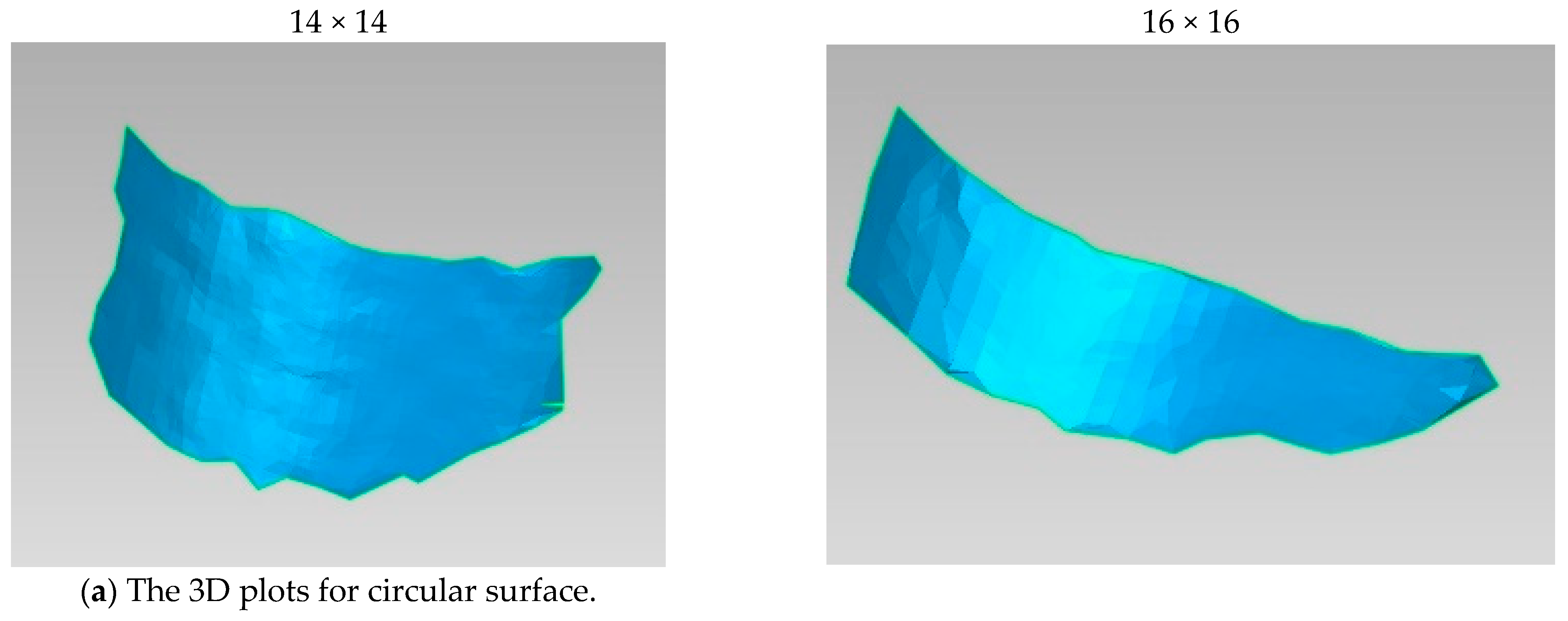
3.3. 3D Plots and Point Clouds of Measuring Surfaces

After applying the techniques described in the previous section, the 3D of simple and complex surfaces, such as cylindrical objects and sculptures, are measured at the accuracy level of 3.1 mm for 14 × 14 pattern resolution and 3.5 mm for 16 × 16 pattern resolution. Figure 14 shows 3D point clouds. Figure 15 shows the 3D reconstruction or 3D plots obtained from 3D point clouds.
The 3D plots and point clouds show more dense reconstruction when compared to our previous method, Ahsan [33]. The points are closer to each other. The point cloud of 14 × 14 resolution is denser than 16 × 16 resolution. The graphical representation of point clouds shows that all points lie between 800 mm and 900 mm in depth or Z-axis. The points displayed in the point clouds are not the same number of classified or decoded stripes. The points that have established correspondence or satisfied the window property of the M-array are included in the point cloud. So, we may miss at least two rows of points near each boundary. Since the proposed method is based on grid coding, which combines the advantages of the simple point and the line, sharp discontinuities may indicate abrupt changes at several points on the object’s surface. However, grid coding implies weak constrictions on the physical entities [77], since labeling intersecting points of the grid is time-consuming; consecutively, some parts of an object are occluded [34]. So, the number of points matched in correspondence for the original pattern is 92%, and simple or circular surfaces are 85% to 87% of stripes classified or decoded. The number of points that establish correspondence for complex surfaces such as sculptures is only 66% to 70% at most.

3.4. Results of Time Calculations

Table 7 shows the time durations for different processes involved during decoding. Each method has a specific time duration. The time durations are measured on the average core i5 computer for various functions. The time calculations are based on average times for each procedure, whereas each event optimizes and is processed many times to obtain optimum results. The time measurements are specified in the units of milliseconds. We also compared the time durations of each function with the time durations consumed for computing single-centroid-based symbols in our previous work [33].
The preprocessing time increases with the complexity of the surface, while it decreases with the decrease in detected primitives. Compared to our previous work, cited at [33], the preprocessing time is much less. This is mainly because stripe patterns are simple and need less time for preprocessing. The preprocessing time for patterns initially projected and simple surfaces is also decreasing compared to complex or textured surfaces such as sculptures or cylinders. A similar phenomenon is observed in labeling, calculating shape description parameters, classifying symbols, and establishing correspondence.
The correspondence rate increases with the complexity and texture of the surface. The matching rate is lower on simple surfaces than textured and complex surfaces. The correspondence time and matching rates are significantly increased compared to our previous work [33]. It is mainly because of the computation of two additional tasks, i.e., stripe indexing and grid adjustments.

4. Conclusions

In this research, we combined two methods, the time-multiplexing stripe indexing method with the single-shot pseudo-random sequence-based method. As a result, the measuring resolution of the pseudo-random sequence-based strategy improved significantly. We proposed a multi-resolution 3D measurement system by defining horizontal and vertical stripes in pixel sizes ranging from 8 × 8 to 16 × 16 pixels. We used robust pseudo-random sequences to spread these stripes in the pattern controllably. We utilized multiple stripes instead of single-shape primitive symbols in the projection pattern since single-shape primitive alphabets or symbols contribute only one feature point. In contrast, various stripes contribute multiple feature points. So, we obtained a single-shot, high-resolution measurement using horizontal and vertical stripes. Due to the employment of simple stripes, the algorithm improves the time durations consumed for preprocessing, such as filtering, thresholding, and labeling. Our technique also shows improvements in decoded or classified feature points compared to the previous methods. Our approach has surpassed all the previous single-shot methods when resolution is compared (the resolution comparison is provided in Table 5). We achieved a measuring pattern resolution of 3.1 mm using a 14 × 14 pattern at a depth of 80 cm. In contrast, the earlier methods, such as Albiter (2007) utilizing a geometric-symbol-based approach, achieve a resolution of 12 mm. Chen (2008) employed a color-coded pseudo-random scheme that achieved a resolution of 10.4 mm. F. Li (2021), utilizing an M-array-based method, achieved a resolution of 8.2 mm. Wijenayake (2012) used two pseudo-random sequences to attain a resolution of 7.4 mm. Bin Liu (2022) employed a stripe-indexed-based method to achieve a resolution of 20.6 mm. Zhou (2023) used a larger M-array to attain a resolution of 8.5 mm. Similarly, our previous work, Ahsan (2020), employing geometric-based symbols, achieved a resolution of 6.6 mm. So, the 3D of simple and complex surfaces, such as cylindrical objects and sculptures, are measured at the resolution of 3.1 mm for the 14 × 14 pattern and 3.5 mm for the 16 × 16 pattern. We implemented a decoding method based on stripe classification, indexing, and grid adjustments. Due to the multiple stripe strategy, the price is paid in computation as correspondence time and rate of matching have increased. However, this cost compensates in terms of significant improvement in measuring resolution.

Author Contributions

Conceptualization, A.E. and Q.Z.; methodology, A.E. and J.L.; software, A.E. and Z.H.; validation, A.E. and J.L.; formal analysis, A.E., J.L. and M.B.; investigation, A.E.; resources, Q.Z. and Y.L.; data curation, A.E. and J.L.; writing—original draft preparation, A.E.; writing—review and editing, A.E. and J.L.; visualization, A.E. and M.B.; supervision, Q.Z.; project administration, Q.Z.; funding acquisition, Q.Z. All authors have read and agreed to the published version of the manuscript.

Funding

National Natural Science Foundation of China with project grant number 52171299.

Data Availability Statement

The research data will be publically available at GIT hub repository.

Conflicts of Interest

The authors declare no conflict of interest.

References

  1. Lyu, B.; Tsai, M.; Chang, C. Infrared Structure Light Projector Design for 3D Sensing. In Proceedings of the Conference on Optical Design and Engineering VII (SPIE Optical Systems Design), Frankfurt, Germany, 14–17 May 2018; Mazuray, L., Mazuray, L., Wartmann, R., Wartmann, R., Wood, A.P., Wood, A., Eds.; SPIE: Frankfurt, Germany, 2018. [Google Scholar]
  2. Albitar, C.; Graebling, P.; Doignon, C. Robust Structured Light Coding for 3D Reconstruction. In Proceedings of the 11th IEEE International Conference on Computer Vision, Rio de Janeiro, Brazil, 14–21 October 2007; IEEE: Rio De Janeiro, Brazil, 2007; pp. 7–12. [Google Scholar]
  3. Yang, L.; Liu, Y.; Peng, J. Advances Techniques of the Structured Light Sensing in Intelligent Welding Robots: A Review. Adv. Manuf. Technol. 2020, 110, 1027–1046. [Google Scholar] [CrossRef]
  4. He, Q.; Zhang, X.; Ji, Z.; Gao, H.; Yang, G. A Novel and Systematic Signal Extraction Method for High-Temperature Object Detection via Structured Light Vision. IEEE Trans. Instrum. Meas. 2022, 71, 1–14. [Google Scholar] [CrossRef]
  5. Drouin, M.-A.; Beraldin, J.-A. Active Triangulation 3D Imaging Systems for Industrial Inspection. In 3D Imaging, Analysis and Applications; Liu, Y., Pears, N., Rosin, P.L., Huber, P., Eds.; Springer Nature: Ottawa, ON, Canada, 2020; pp. 109–165. [Google Scholar]
  6. Molleda, J.; Usamentiaga, R.; Garcıa, D.F.; Bulnes, F.G.; Espina, A.; Dieye, B.; Smith, L.N. An Improved 3D Imaging System for Dimensional Quality Inspection of Rolled Products in the Metal Industry. Comput. Ind. 2013, 64, 1186–1200. [Google Scholar] [CrossRef]
  7. Zhang, C.; Zhao, C.; Huang, W.; Wang, Q.; Liu, S.; Li, J.; Guo, Z. Automatic Detection of Defective Apples Using NIR Coded Structured Light and Fast Lightness Correction. J. Food Eng. 2017, 203, 69–82. [Google Scholar] [CrossRef]
  8. Salvi, J.; Fernandez, S.; Pribanic, T.; Llado, X. A State of the Art in Structured Light Patterns for Surface Profilometry. Pattern Recognit. 2010, 43, 2666–2680. [Google Scholar] [CrossRef]
  9. Webster, J.G.; Bell, T.; Li, B.; Zhang, S. Structured Light Techniques and Applications. Wiley Encycl. Electr. Electron. Eng. 2016, 1–24. [Google Scholar] [CrossRef]
  10. Zhang, S. High-Speed 3D Shape Measurement with Structured Light Methods: A Review. Opt. Lasers Eng. 2018, 106, 119–131. [Google Scholar] [CrossRef]
  11. Salvi, J.; Pagès, J.; Batlle, J. Pattern Codification Strategies in Structured Light Systems. Pattern Recognit. 2004, 37, 827–849. [Google Scholar] [CrossRef]
  12. Villena-martínez, V.; Fuster-guilló, A.; Azorín-lópez, J.; Saval-calvo, M.; Mora-pascual, J.; Garcia-rodriguez, J.; Garcia-garcia, A. A Quantitative Comparison of Calibration Methods for RGB-D Sensors Using Different Technologies. Sensors 2017, 17, 243. [Google Scholar] [CrossRef]
  13. Hall-Holt, O.; Rusinkiewicz, S. Stripe Boundary Codes for Real-Time Structured-Light Range Scanning of Moving Objects. In Proceedings of the IEEE International Conference on Computer Vision 2001, Vancouver, BC, Canada, 7–14 July 2001; Volume 2, pp. 359–366. [Google Scholar] [CrossRef]
  14. Rusinkiewicz, S.; Hall-Holt, O.; Levoy, M. Real-Time 3D Model Acquisition. ACM Trans. Graph. 2002, 21, 438–446. [Google Scholar] [CrossRef]
  15. Nguyen, H.; Wang, Y.; Wang, Z. Single-Shot 3D Shape Reconstruction Using Structured Light and Deep Convolutional Neural Networks. Sensors 2020, 20, 3718. [Google Scholar] [CrossRef]
  16. Pan, B.; Xie, H.; Gao, J.; Asundi, A. Improved Speckle Projection Profilometry for Out-of-Plane Shape Measurement. Appl. Opt. 2008, 47, 5527–5533. [Google Scholar] [CrossRef]
  17. Posdamer, J.L.; Altschuler, M.D. Surface Measurement by Space-Encoded Projected Beam Systems. Comput. Graph. Image Process. 1982, 18, 1–17. [Google Scholar] [CrossRef]
  18. Gühring, J. Dense 3-D Surface Acquisition by Structured Light Using off-the-Shelf Components. In Proceedings of the SPIE Proceedings 4309, Videometrics and Optical Methods for 3D Shape Measurement, San Jose, CA, USA, 22–23 January 2001; SPIE: San Jose, CA, USA, 2001. [Google Scholar]
  19. Er, M.C. On Generating the N-Ary Reflected Gray Codes. IEEE Trans. Comput. 1984, 33, 739–741. [Google Scholar] [CrossRef]
  20. Horn, E.; Kiryati, N. Toward Optimal Structured Light Patterns. Image Vis. Comput. 1999, 17, 87–97. [Google Scholar] [CrossRef]
  21. Liu, B.; Yang, F.; Huang, Y.; Zhang, Y.; Wu, G. Single-Shot Three-Dimensional Reconstruction Using Grid Pattern-Based Structured-Light Vision Method. Appl. Sci. 2022, 12, 10602. [Google Scholar] [CrossRef]
  22. Durdle, N.G.; Thayyoor, J.; Raso, V.J. An Improved Structured Light Technique for Surface Reconstruction of the Human Trunk. In Proceedings of the IEEE Canadian Conference on Electrical and Computer Engineering, Waterloo, ON, Canada, 25–28 May 1998; IEEE: Waterloo, ON, Canada, 1998; pp. 874–877. [Google Scholar]
  23. Maruyama, M.; Abe, S. Range Sensing by Projecting Multiple Slits with Random Cuts. IEEE Trans. Pattern Anal. Mach. Intell. 1993, 15, 647–651. [Google Scholar] [CrossRef]
  24. Je, C.; Lee, S.W.; Park, R.H. High-Contrast Color-Stripe Pattern for Rapid Structured-Light Range Imaging. In Proceedings of the Eighth European Conference on Computer Vision (ECCV), Prague, Czech Republic, 11–14 May 2004; Lecture Notes in Computer Science; Springer: Berlin/Heidelberg, Germany, 2004; Volume 3021, pp. 95–107. [Google Scholar]
  25. Je, C.; Lee, S.W.; Park, R.H. Colour-Stripe Permutation Pattern for Rapid Structured-Light Range Imaging. Opt. Commun. 2012, 285, 2320–2331. [Google Scholar] [CrossRef]
  26. Ahsan, E.; QiDan, Z.; Jun, L.; Yong, L.; Muhammad, B. Grid-Indexed Based Three-Dimensional Profilometry. In Coded Optical Imaging; Liang, D.J., Ed.; Springer Nature: Ottawa, ON, Canada, 2023. [Google Scholar]
  27. Zuo, C.; Feng, S.; Huang, L.; Tao, T.; Yin, W.; Chen, Q. Phase Shifting Algorithms for Fringe Projection Profilometry: A Review. Opt. Lasers Eng. 2018, 109, 23–59. [Google Scholar] [CrossRef]
  28. Ito, M.; Ishii, A. A Three-Level Checkerboard Pattern (TCP) Projection Method for Curved Surface Measurement. Pattern Recognit. 1995, 28, 27–40. [Google Scholar] [CrossRef]
  29. Hugli, H.; Maitre, G. Generation And Use Of Color Pseudo Random Sequences For Coding Structured Light In Active Ranging. Ind. Insp. 2012, 1010, 75. [Google Scholar] [CrossRef]
  30. Pagès, J.; Salvi, J.; Collewet, C.; Forest, J. Optimised de Bruijn Patterns for One-Shot Shape Acquisition. Image Vis. Comput. 2005, 23, 707–720. [Google Scholar] [CrossRef]
  31. Zhang, L.; Curless, B.; Seitz, S.M. Rapid Shape Acquisition Using Color Structured Light and Multi-Pass Dynamic Programming. In Proceedings of the Proceedings—1st International Symposium on 3D Data Processing Visualization and Transmission, 3DPVT 2002, Padova, Italy, 19–21 June 2002; IEEE Computer Society: Montreal, QC, Canada, 2002; pp. 24–36. [Google Scholar]
  32. Ha, M.; Xiao, C.; Pham, D.; Ge, J. Complete Grid Pattern Decoding Method for a One-Shot Structured Light System. Appl. Opt. 2020, 59, 2674–2685. [Google Scholar] [CrossRef]
  33. Elahi, A.; Lu, J.; Zhu, Q.D.; Yong, L. A Single-Shot, Pixel Encoded 3D Measurement Technique for Structure Light. IEEE Access 2020, 8, 127254–127271. [Google Scholar] [CrossRef]
  34. Morano, R.A.; Ozturk, C.; Conn, R.; Dubin, S.; Zietz, S.; Nissanov, J. Structured Light Using Pseudorandom Codes. IEEE Trans. Pattern Anal. Mach. Intell. 1998, 20, 322–327. [Google Scholar] [CrossRef]
  35. Lu, J.; Han, J.; Ahsan, E.; Xia, G.; Xu, Q. A Structured Light Vision Measurement with Large Size M-Array for Dynamic Scenes. In Proceedings of the 35th Chinese Control Conference (CCC), Chengdu, China, 27–29 July 2016; IEEE: Chengdu, China, 2016; pp. 3834–3839. [Google Scholar]
  36. Chen, S.Y.; Li, Y.F.; Zhang, J. Vision Processing for Realtime 3-D Data Acquisition Based on Coded Structured Light. IEEE Trans. Image Process. 2008, 17, 167–176. [Google Scholar] [CrossRef]
  37. Li, F.; Shang, X.; Tao, Q.; Zhang, T.; Shi, G.; Niu, Y. Single-Shot Depth Sensing with Pseudo Two-Dimensional Sequence Coded Discrete Binary Pattern. IEEE Sens. J. 2021, 21, 11075–11083. [Google Scholar] [CrossRef]
  38. Wijenayake, U.; Choi, S.I.; Park, S.Y. Combination of Color and Binary Pattern Codification for an Error Correcting M-Array Technique. In Proceedings of the 2012 9th Conference on Computer and Robot Vision, CRV 2012, Toronto, ON, Canada, 28–30 May 2012; pp. 139–146. [Google Scholar] [CrossRef]
  39. Yin, W.; Cao, L.; Zhao, H.; Hu, Y.; Feng, S.; Zhang, X.; Shen, D.; Wang, H.; Chen, Q.; Zuo, C. Real-Time and Accurate Monocular 3D Sensor Using the Reference Plane Calibration and an Optimized SGM Based on Opencl Acceleration. Opt. Lasers Eng. 2023, 165. [Google Scholar] [CrossRef]
  40. Yin, W.; Hu, Y.; Feng, S.; Huang, L.; Kemao, Q.; Chen, Q.; Zuo, C. Single-Shot 3D Shape Measurement Using an End-to-End Stereo Matching Network for Speckle Projection Profilometry. Opt. Express 2021, 29, 13388. [Google Scholar] [CrossRef]
  41. Yin, W.; Feng, S.; Tao, T.; Huang, L.; Trusiak, M.; Chen, Q.; Zuo, C. High-Speed 3D Shape Measurement Using the Optimized Composite Fringe Patterns and Stereo-Assisted Structured Light System. Opt. Express 2019, 27, 2411. [Google Scholar] [CrossRef]
  42. Petriu, E.M.; Sakr, Z.; Spoelder, H.J.W.; Moica, A. Object Recognition Using Pseudo-Random Color Encoded Structured Light. In Proceedings of the 17th IEEE Instrumentation and Measurement Technology Conference, Baltimore, MD, USA, 1–4 May 2000; IEEE: Baltimore, MD, USA, 2000; pp. 1237–1241. [Google Scholar]
  43. Salvi, J.; Batlle, J.; Mouaddib, E. A Robust-Coded Pattern Projection for Dynamic 3D Scene Measurement. Pattern Recognit. Lett. 1998, 19, 1055–1065. [Google Scholar] [CrossRef]
  44. Griffin, P.M.; Narasimhan, L.S.; Yee, S.R. Generation of Uniquely Encoded Light Patterns for Range Data Acquisition. Pattern Recognit. 1992, 25, 609–616. [Google Scholar] [CrossRef]
  45. Desjardins, D.; Payeur, P. Dense Stereo Range Sensing with Marching Pseudo-Random Patterns. In Proceedings of the Proceedings—Fourth Canadian Conference on Computer and Robot Vision, CRV 2007, Montreal, QC, Canada, 28–30 May 2007; IEEE Computer Society: Montreal, QC, Canada, 2007; pp. 216–223. [Google Scholar]
  46. Payeur, P.; Desjardins, D. Structured Light Stereoscopic Imaging with Dynamic Pseudo-Random Patterns. In 6th International Conference, ICIAR 2009, Halifax, Canada, 6–8 July 2009; Lecture Notes in Computer Science; Springer: Berlin/Heidelberg, Germany, 2009; Volume 5627, pp. 687–696. [Google Scholar]
  47. Chen, S.Y.; Li, Y.F.; Zhang, J. Realtime Structured Light Vision with the Principle of Unique Color Codes. Proc. IEEE Int. Conf. Robot. Autom. 2007, 429–434. [Google Scholar] [CrossRef]
  48. Song, Z.; Chung, R. Grid Point Extraction Exploiting Point Symmetry in a Pseudo-Random Color Pattern. In Proceedings of the 15th IEEE International Conference of Image Processing, San Diego, CA, USA, 12–15 October 2008; IEEE: San Diego, CA, USA, 2008; pp. 1956–1959. [Google Scholar]
  49. Song, Z.; Chung, R. Determining Both Surface Position and Orientation in Structured-Light-Based Sensing. IEEE Trans. Pattern Anal. Mach. Intell. 2010, 32, 1770–1780. [Google Scholar] [CrossRef]
  50. Lin, H.; Nie, L.; Song, Z. A Single-Shot Structured Light Means by Encoding Both Color and Geometrical Features. Pattern Recognit. 2016, 54, 178–189. [Google Scholar] [CrossRef]
  51. Shi, G.; Li, R.; Li, F.; Niu, Y.; Yang, L. Depth Sensing with Coding-Free Pattern Based on Topological Constraint. J. Vis. Commun. Image Represent. 2018, 55, 229–242. [Google Scholar] [CrossRef]
  52. Albitar, C.; Graebling, P.; Doignon, C. Design of a Monocular Pattern for a Robust Structured Light Coding. In Proceedings of the IEEE International Conference on Image Processing, San Antonio, TX, USA, 16 September–19 October 2007; IEEE: San Antonio, TX, USA, 2007; pp. 529–532. [Google Scholar]
  53. Lei, Y.; Bengtson, K.R.; Li, L.; Allebach, J.P. Design and Decoding of an M-Array Pattern for Low-Cost Structured 3D Reconstruction Systems. In Proceedings of the 2013 IEEE International Conference on Image Processing, Melbourne, VIC, Australia, 15–18 September 2013; pp. 2168–2172. [Google Scholar]
  54. Tang, S.; Zhang, X.; Song, Z.; Jiang, H.; Nie, L. Three-Dimensional Surface Reconstruction via a Robust Binary Shape-Coded Structured Light Method. Opt. Eng. 2017, 56, 014102. [Google Scholar] [CrossRef]
  55. Zhou, X.; Zhou, C.; Kang, Y.; Zhang, T.; Mou, X. Pattern Encoding of Robust M-Array Driven by Texture Constraints. IEEE Trans. Instrum. Meas. 2023, 72, 5014816. [Google Scholar] [CrossRef]
  56. Gu, F.; Du, H.; Wang, S.; Su, B.; Song, Z. High-Capacity Spatial Structured Light for Robust and Accurate Reconstruction. Sensors 2023, 23, 4685. [Google Scholar] [CrossRef]
  57. Zhao, Z.; Xin, B.; Li, L.; Huang, Z.-L. High-Power Homogeneous Illumination for Super-Resolution Localization Microscopy with Large Field-of-View. Opt. Express 2017, 25, 13382. [Google Scholar] [CrossRef]
  58. Savage, N. Digital Spatial Light Modulator. Nat. Photonics 2009, 3, 170–172. [Google Scholar] [CrossRef]
  59. Neff, J.A.; Athale, R.A.; Lee, S.H. Two-Dimensional Spatial Light Modulators: A Tutorial. Proc. IEEE 1990, 78, 826–855. [Google Scholar] [CrossRef]
  60. Bui, L.Q.; Lee, S. A Method of Eliminating Interreflection in 3D Reconstruction Using Structured Light 3D Camera The Appearance of Interreflection. In Proceedings of the 2014 9th International Conference on Computer Vision, Theory and Applications (Visapp 2014), Lisbon, Portugal, 5–8 January 2014; IEEE: Lisbon, Portugal, 1993; Volume 3. [Google Scholar]
  61. Nguyen, H.; Ly, K.L.; Li, C.Q.; Wang, Z. Single-Shot 3D Shape Acquisition Using a Learning-Based Structured-Light Technique. Appl. Opt. 2022, 61, 8589–8599. [Google Scholar] [CrossRef] [PubMed]
  62. Wang, L.; Lu, D.; Qiu, R.; Tao, J. 3D Reconstruction from Structured-light Profilometry with Dual-path Hybrid Network. EURASIP J. Adv. Signal Process. 2022, 2022, 14. [Google Scholar] [CrossRef]
  63. Nguyen, H.; Wang, Z. Accurate 3D Shape Reconstruction from Single Structured-Light Image via Fringe-to-Fringe Network. Photonics 2021, 8, 459. [Google Scholar] [CrossRef]
  64. Xtion, A.; Realsense, I. MIMONet: Structured-Light 3D Shape Reconstruction by a Multi-Input Multi-Output Network. Appl. Opt. 2021, 60, 5134–5144. [Google Scholar] [CrossRef]
  65. Tang, S.; Song, L.; Zeng, H. Robust Pattern Decoding in Shape-Coded Structured Light. Opt. Lasers Eng. 2017, 96, 50–62. [Google Scholar] [CrossRef]
  66. Guo, Y.; Liu, Y.; Oerlemans, A.; Lao, S.; Wu, S.; Lew, M.S. Deep Learning for Visual Understanding: A Review. Neurocomputing 2016, 187, 27–48. [Google Scholar] [CrossRef]
  67. Kurnianggoro, L.; Wahyono; Jo, K.H. A Survey of 2D Shape Representation: Methods, Evaluations, and Future Research Directions. Neurocomputing 2018, 300, 1–16. [Google Scholar] [CrossRef]
  68. Yang, M.; Kpalma, K.; Ronsin, J. A Survey of Shape Feature Extraction Techniques. Pattern Recognit. 2008, 15, 43–90. [Google Scholar]
  69. Sezgin, M.; Sankur, B. Survey over Image Thresholding Techniques and Quantitative Performance Evaluation. J. Electron. Imaging 2004, 13, 146–165. [Google Scholar] [CrossRef]
  70. Haralick, R.M.; Shapiro, L.G. Computer and Robot Vision Volume 1; Addison-Wesley Publishing Company: Boston, MA, USA, 1992; ISBN 0201108771. [Google Scholar]
  71. Gonzalez, R.C.; Woods, R.E. Digital Image Processing; Pearson International Edition Prepared by Pearson Education; Prentice Hall: Kent, OH, USA, 2009; pp. 861–877. [Google Scholar] [CrossRef]
  72. Sonka, M.; Hlavac, V.; Boyle, R. Image Processing, Analysis, and Machina Vision, 3rd ed.; Thomson: Toronto, ON, Canada, 2008; ISBN 978-0-495-08252-1. [Google Scholar]
  73. Xie, Z.; Wang, X.; Chi, S. Simultaneous Calibration of the Intrinsic and Extrinsic Parameters of Structured-Light Sensors. Opt. Lasers Eng. 2014, 58, 9–18. [Google Scholar] [CrossRef]
  74. Nie, L.; Ye, Y.; Song, Z. Method for Calibration Accuracy Improvement of Projector-Camera-Based Structured Light System. Opt. Eng. 2017, 56, 074101. [Google Scholar] [CrossRef]
  75. Huang, B.; Ozdemir, S.; Tang, Y.; Liao, C.; Ling, H. A Single-Shot-Per-Pose Camera-Projector Calibration System for Imperfect Planar Targets. In Proceedings of the Adjunct Proceedings—2018 IEEE International Symposium on Mixed and Augmented Reality, ISMAR-Adjunct 2018, Munich, Germany, 16–20 October 2018; pp. 15–20. [Google Scholar] [CrossRef]
  76. Moreno, D.; Taubin, G. Simple, Accurate, and Robust Projector-Camera Calibration. In Proceedings of the 2nd Joint 3DIM/3DPVT Conference: 3D Imaging, Modeling, Processing, Visualization and Transmission, 3DIMPVT 2012, Zurich, Switzerland, 13–15 October 2012; pp. 464–471. [Google Scholar] [CrossRef]
  77. Hu, G.; Stockman, G. 3-D Surface Solution Using Structured Light and Constraint Propagation. IEEE Trans. Pattern Anal. Mach. Intell. 1989, 11, 390–402. [Google Scholar] [CrossRef]
Figure 1. Stripes vary in size from 8 × 8 to 16 × 16 pixels.
Photonics 10 01212 g001
Figure 2. The Hamming distance profiles of various M-arrays. Note: Each M-array has seven alphabets.
Photonics 10 01212 g002
Figure 3. (ae), Parts of projection patterns for single-centroid symbols from previous approaches [34]. (fj), Parts of proposed projection patterns employing strip-based approach.
Photonics 10 01212 g003
Figure 4. Comparison of the number of feature points. Note: The number of feature points increases by a factor of two or more for each resolution in the stripe pattern.
Photonics 10 01212 g004
Figure 5. The process of searching in the neighborhood. The scanning is performed 0.9 times the grid distance for stripe types 2 and 3. The scanning is performed multiple times of grid distance in the case of stripe types 6 and 7 till a different stripe is found in the neighborhood. The upper circle shows searching on the right side of the neighborhood. The lower circle shows searching in the downside of the neighborhood.
Photonics 10 01212 g005
Figure 6. Procedure to find stripe indexes and grid adjustments: (a) Stripe type 2, (b) stripe type 3, and (c) grid adjustments. Note: Scanning is performed 0.9 times the grid distance. Stripe types 2 and 3 occur in modulo of two stripes. The index is decided after calculating the distance from the neighborhood stripe. If the calculated distance exceeds 0.5 times the grid distance, the stripe is indexed as part 2. If the calculated distance is less than 0.5 times the neighborhood stripe, the stripe is marked as part 1.
Photonics 10 01212 g006
Figure 7. Method to find the stripe indexes and grid adjustments: (a) Stripe type 7 with forward stripe indexing strategy, (b) stripe type 6 with backward stripe indexing strategy, and (c) grid adjustment. Note: Scanning is performed multiple times till a different type of stripe occurs in the vicinity. The index is calculated by counting the number of stripes from that different stripe found in the neighborhood.
Photonics 10 01212 g007
Figure 8. Finding or calculating the neighborhood stripes to establish correspondence. The blue lines show the grid distance between the consecutive neighborhood stripes. The current stripe’s adjusted centroid position and neighborhood stripes’ calculated centroid position are shown with red dots on blue lines. The segmented red lines show the lines parallel to the X and Y axes.
Photonics 10 01212 g008
Figure 9. The camera, projector devices, and the objects that were used for measurement in the experiment.
Photonics 10 01212 g009
Figure 10. The schema of the projector and camera position with respect to the target object.
Photonics 10 01212 g010
Figure 11. Textured part of stripe patterns employed in the experiment.
Photonics 10 01212 g011
Figure 12. Classification of stripes in the original and simple surface.
Photonics 10 01212 g012
Figure 13. Classification of stripes in the cylindrical and sculpture surface.
Photonics 10 01212 g013
Figure 14. The 3D Point Clouds.
Photonics 10 01212 g014
Figure 15. The 3D reconstruction results.
Photonics 10 01212 g015aPhotonics 10 01212 g015b
Table 1. Properties of M-arrays for various resolutions.
Stripe SizeSpacing between Consecutive SymbolsNo. of Symbols Used in M-ArrayM-Array Dimensions (m × n)Average Hamming DistanceRobust Codewords (%)
8 × 81790 × 1447.713799.9963
10 × 102769 × 1087.71499.9968
12 × 122760 × 937.714399.9964
14 × 142751 × 817.71999.9971
16 × 162745 × 727.718699.9954
Table 2. Feature point calculations for various resolution.
Pattern Resolution (Sres)Feature PointsIncrease in Feature Points Ratio (α)Increase in Feature Points (%)
Single-Centroid Symbols Strips Based Projection
8 × 8 pixel12,49626,7012.1368113.68
10 × 10 pixel699616,7892.3998139.98
12 × 12 pixel518713,9252.6846168.46
14 × 14 pixel400085692.1423114.22
16 × 16 pixel312466562.1306113.06
Table 3. Stripe classification parameters.
SymbolParameterDefinition
EEccentricity μ 20 + μ 02 μ 20 μ 02 2 + 4 μ 11 2 μ 20 + μ 02 + μ 20 μ 02 2 + 4 μ 11 2
ARAspect ratio M a j o r A x i s M i n o r A x i s
PARPerimeter to Area P S A S
CRCircularity or Compactness A S A C I R
4 π A S P S 2
x ¯ , y ¯ Centroid 1 N 1 N x i , 1 N y i or
m 10 m 00 ,   m 01 m 00  
θ Orientation 1 2 arctan ( 2 μ 11 μ 20 μ 02 )
gridGrid DistanceMajor axis + Sspace
where μ 11 ,   μ 02 ,   μ 20 are the second-order moments along the center, x-axis, and y-axis, respectively. AS in the area of a stripe symbol, Ps is the parameter of a stripe symbol, ACIR is the circle area with the same parameter, N is the total number of pixels in the alphabet, i is the ith position of a pixel in a symbol, m 00 , m 10 , and m 01 are zero-order moments along the center, x-axis, and y-axis, respectively.
Table 4. Calculation of classification parameters.
Stripe TypePixel SizeEARPARθCR
Square-shaped strip
Photonics 10 01212 i001
8 × 8010.4201.00
10 × 100.350.94
12 × 120.300.90
14 × 140.260.87
16 × 160.230.85
Two parallel horizontal stripes
Photonics 10 01212 i002
8 × 80.9740.9600.86
10 × 100.9850.960.68
12 × 120.9740.700.72
14 × 140.984.670.690.63
16 × 160.9740.550.66
Two parallel vertical stripes
Photonics 10 01212 i003
8 × 80.9740.96 π 2 0.86
10 × 100.9850.960.68
12 × 120.9740.700.72
14 × 140.984.670.690.63
16 × 160.9740.550.66
One horizontal strip
Photonics 10 01212 i004
8 × 80.8720.6001.00
10 × 100.922.50.580.86
12 × 120.8720.430.86
14 × 140.902.330.420.80
16 × 160.8720.330.81
One vertical strip
Photonics 10 01212 i005
8 × 80.8720.60 π 2 1.00
10 × 100.922.50.580.86
12 × 120.8720.430.86
14 × 140.902.330.420.80
16 × 160.8720.330.81
Multiple parallel vertical stripes
Photonics 10 01212 i006
8 × 80.9981.72 π 2 0.53
10 × 100.99101.760.40
12 × 121.00121.800.32
14 × 140.9970.970.48
16 × 160.9980.970.42
Multiple parallel horizontal stripes
Photonics 10 01212 i007
8 × 80.9981.7200.53
10 × 100.99101.760.40
12 × 121.00121.800.32
14 × 140.9970.970.48
16 × 160.9980.970.42
Table 5. Comparison of measured resolution and covered area.
Pattern ResolutionDepth (z) cmArea (cm2)Proposed MethodAhsan [33] (2020)Zhou [55] (2023)Bin Liu [21] (2022)F. Li [37] (2021)Nguyen [15] (2020)Yin [40,41] (2019, 2021)Wijenayake [38] (2012)Chen [36,47] (2008)Albiter [2,52] (2007)
Resolution (mm)Resolution (mm)Resolution (mm)Resolution (mm)Resolution (mm)Resolution (mm)Resolution (mm)Resolution (mm)Resolution (mm)Resolution (mm)
8 × 8250103.8 × 1665.511.826.764.7 (area reduced to 103.8 × 103.8)25.941.425.923 (area reduced to 99.3 × 99.3)32.537.5 (area reduced to 103.8 × 111.5)
10 × 106.014.3
12 × 126.316.8
14 × 149.720.8
16 × 1610.923.3
8 × 820083 × 132.84.49.421.351.7 (area reduced to 83 × 83)20.733.120.718.4 (area reduced to 79.4 × 79.4)2630 (area reduced to 83 × 89.2)
10 × 104.811.4
12 × 125.013.4
14 × 147.816.6
16 × 168.718.6
8 × 815062.3 × 99.63.37.116.138.9 (area reduced to 62.3 × 62.3)15.624.915.613.8 (area reduced to 59.6 × 59.6)19.522.5 (area reduced to 62.3 × 66.9)
10 × 103.68.6
12 × 123.810.1
14 × 145.812.5
16 × 166.614
8 × 812049.8 × 79.72.65.612.730.8 (area reduced to 49.8 × 49.8)12.319.712.311 (area reduced to 47.6 × 47.6)15.618 (area reduced to 49.8 × 53.5)
10 × 102.86.8
12 × 123.08
14 × 144.710
16 × 165.211.1
8 × 810041.5 × 66.42.24.710.725.8 (area reduced to 41.5 × 41.5)10.316.510.39.2 (area reduced to 39.7 × 39.7)1315 (area reduced to 41.5 × 44.6)
10 × 102.45.7
12 × 122.56.7
14 × 143.98.3
16 × 164.49.3
8 × 88033.2 × 53.11.83.88.520.6 (area reduced to 33.2 × 33.2)8.213.28.27.4 (area reduced to 31.8 × 31.8)10.412 (area reduced to 33.2 × 53.1)
10 × 101.94.6
12 × 122.05.4
14 × 143.16.6
16 × 163.57.4
8 × 86024.9 × 39.81.32.86.415.6 (area reduced to 24.9 × 24.9)6.210.06.25.5 (area reduced to 23.8 × 23.8)7.89 (area reduced to 24.9 × 26.8)
10 × 101.43.4
12 × 121.54
14 × 142.35
16 × 162.65.6
8 × 84016.6 × 26.60.91.94.210.3 (area reduced to 16.6 × 16.6)4.17.54.13.7 (area reduced to 15.9 × 15.9)5.26 (area reduced to 16.6 × 17.8)
10 × 100.962.3
12 × 121.012.7
14 × 141.53.3
16 × 161.73.7
Table 6. Detected and decoded primitive and comparison.
Surface TypePattern 1 (Primitives)
16 × 16 Resolution,
Depth 80 cm
Pattern 2 (Primitives)
14 × 14 Resolution,
Depth 80 cm
Ahsan (2020)
16 × 16 Resolution,
Depth 200 cm
DetectedDecoded%DetectedDecoded%DetectedDecoded%
Original Pattern665666561008569856910032403240100
Plane40644064100516351631001650161798
Cylinder21832183100261926191001161112897.1
Sculpture1795178899.62319231499.868958584.9
Table 7. The time calculation for different processes of decoding.
Surface TypeMethodResolutionPreprocessing (Filtering + Thresholding)LabelingParameter CalculationClassificationCorrespondenceRate of Correspondence
Original PatternAhsan [33] (2020)16 × 16566425873.34850.19
Proposed Method14 × 1430246.51498.70.33227.60.38
16 × 16215.426.91210.50.32529.30.38
Plane SurfaceAhsan [33] (2020)16 × 1661153365.62.24800.3
Proposed Method14 × 14227.833.511160.22472.60.48
16 × 16225.728.49070.21942.10.48
CylinderAhsan [33] (2020)16 × 1664941.53612.7331.10.29
Proposed Method14 × 14209.316.6544.20.11289.40.49
16 × 16198.515.3466.40.11069.70.49
SculptureAhsan [33] (2020)16 × 16644382712.73180.5
Proposed Method14 × 14198.815.1494.60.11163.30.5
16 × 16200.613.8390.60.1897.50.5
Note: Time measured and specified in milliseconds.
Disclaimer/Publisher’s Note: The statements, opinions and data contained in all publications are solely those of the individual author(s) and contributor(s) and not of MDPI and/or the editor(s). MDPI and/or the editor(s) disclaim responsibility for any injury to people or property resulting from any ideas, methods, instructions or products referred to in the content.

