Polarization Lidar: Principles and Applications


Abstract
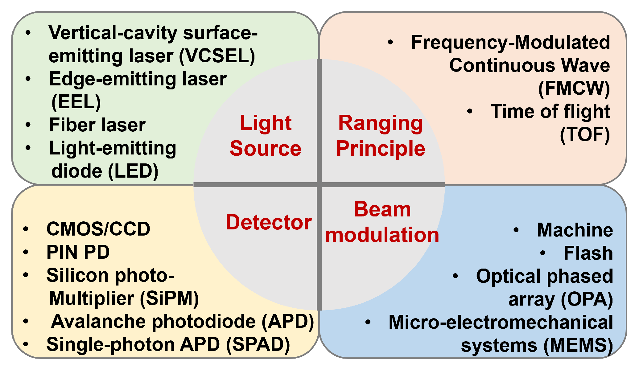
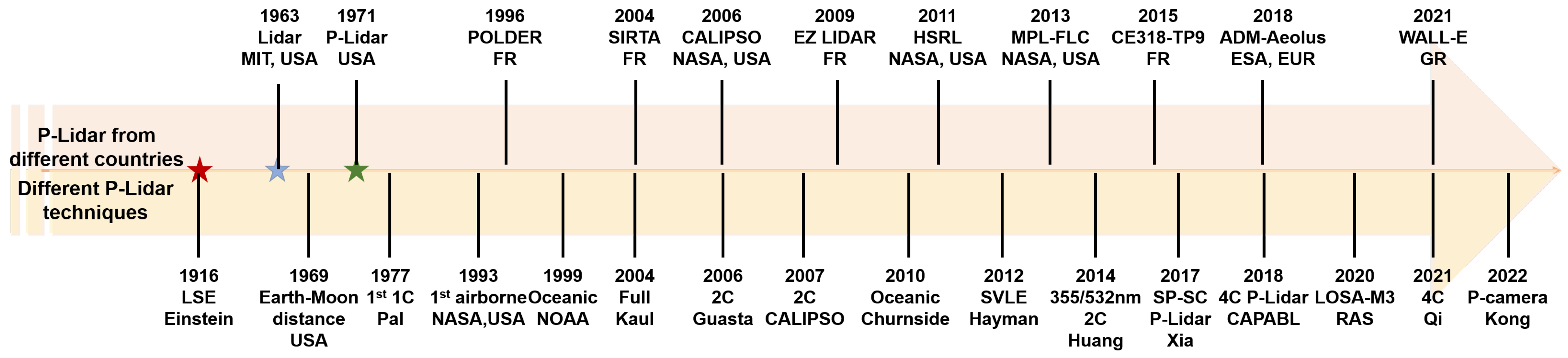
:1. Introduction
2. Principles of Polarization and P-Lidar
2.1. Polarized Light and Its Description
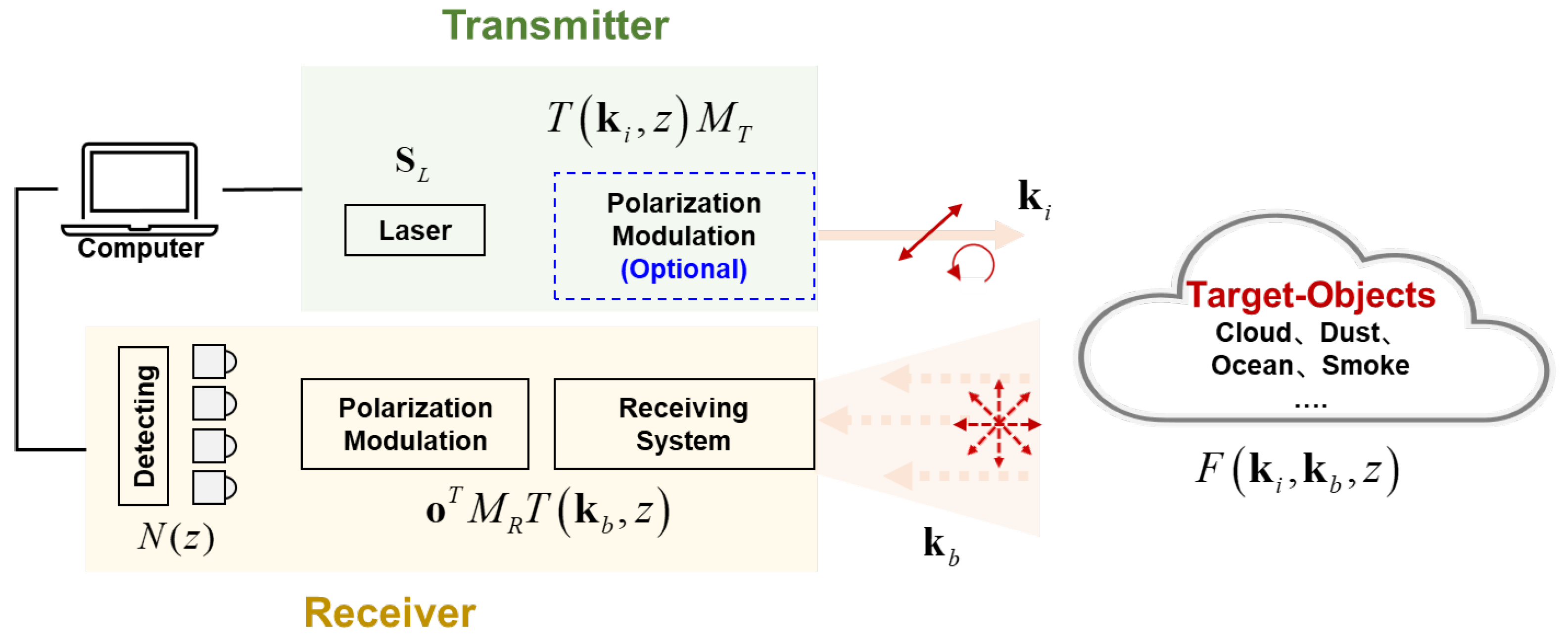
2.2. Principle of P-Lidar
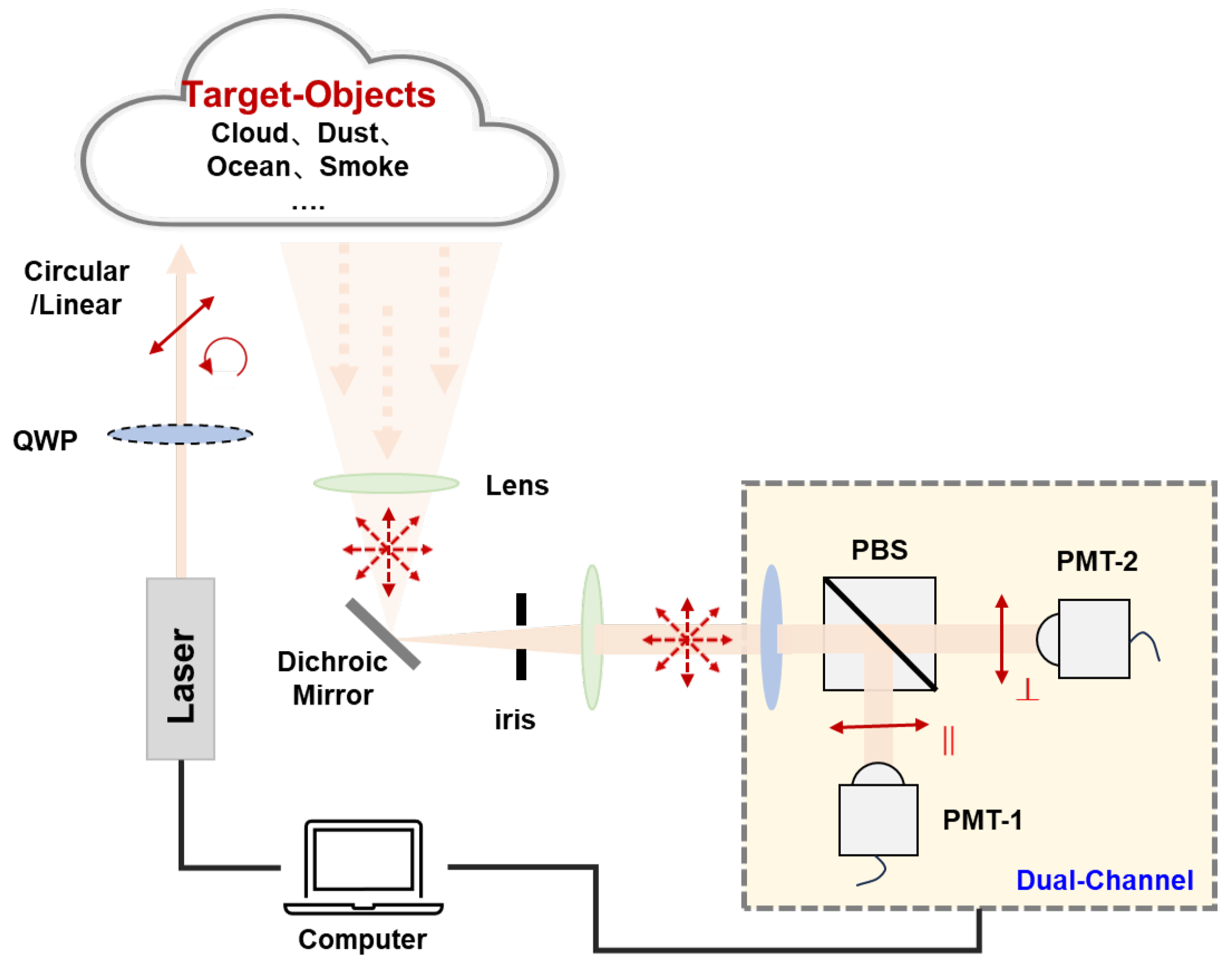
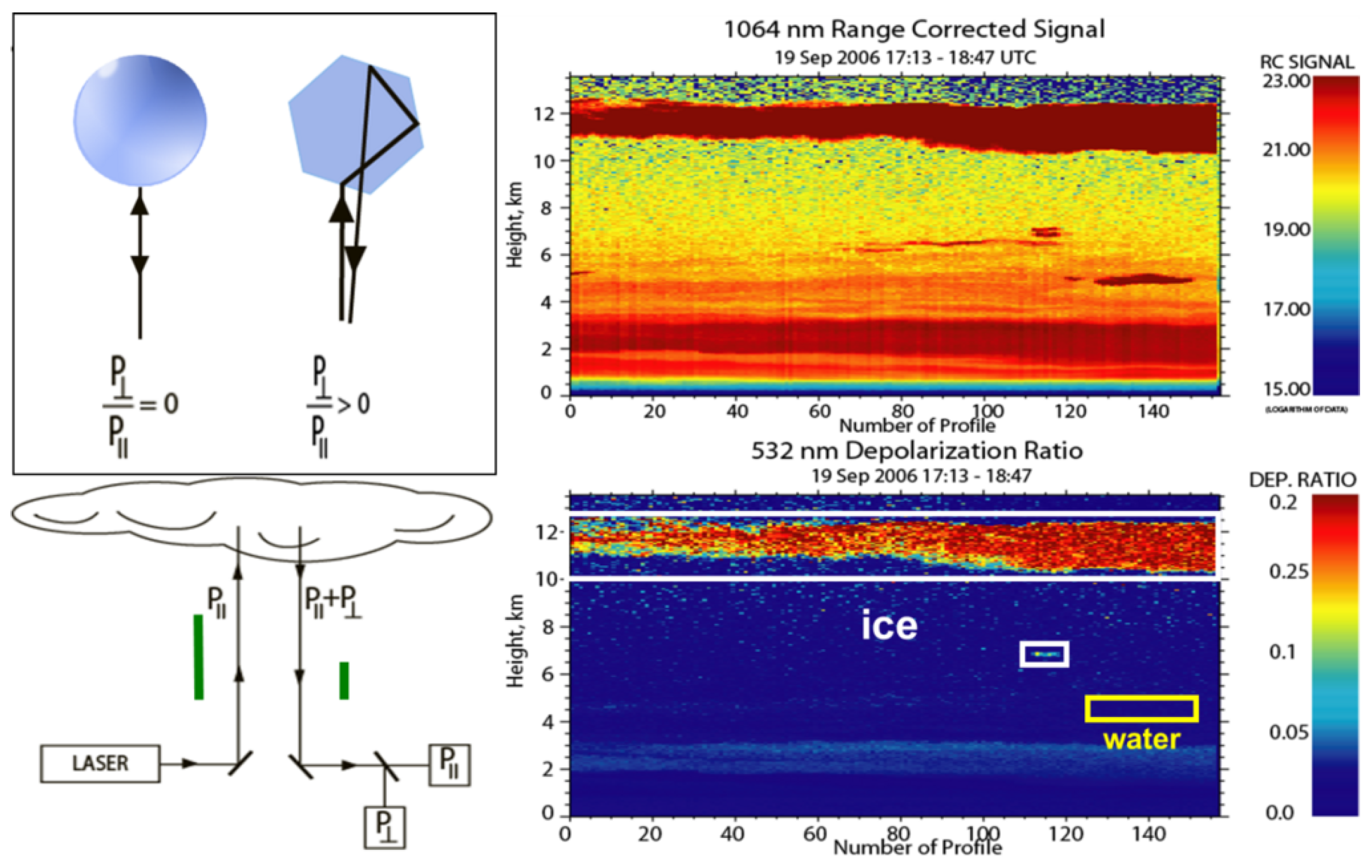
2.2.1. Dual-Channel P-Lidar
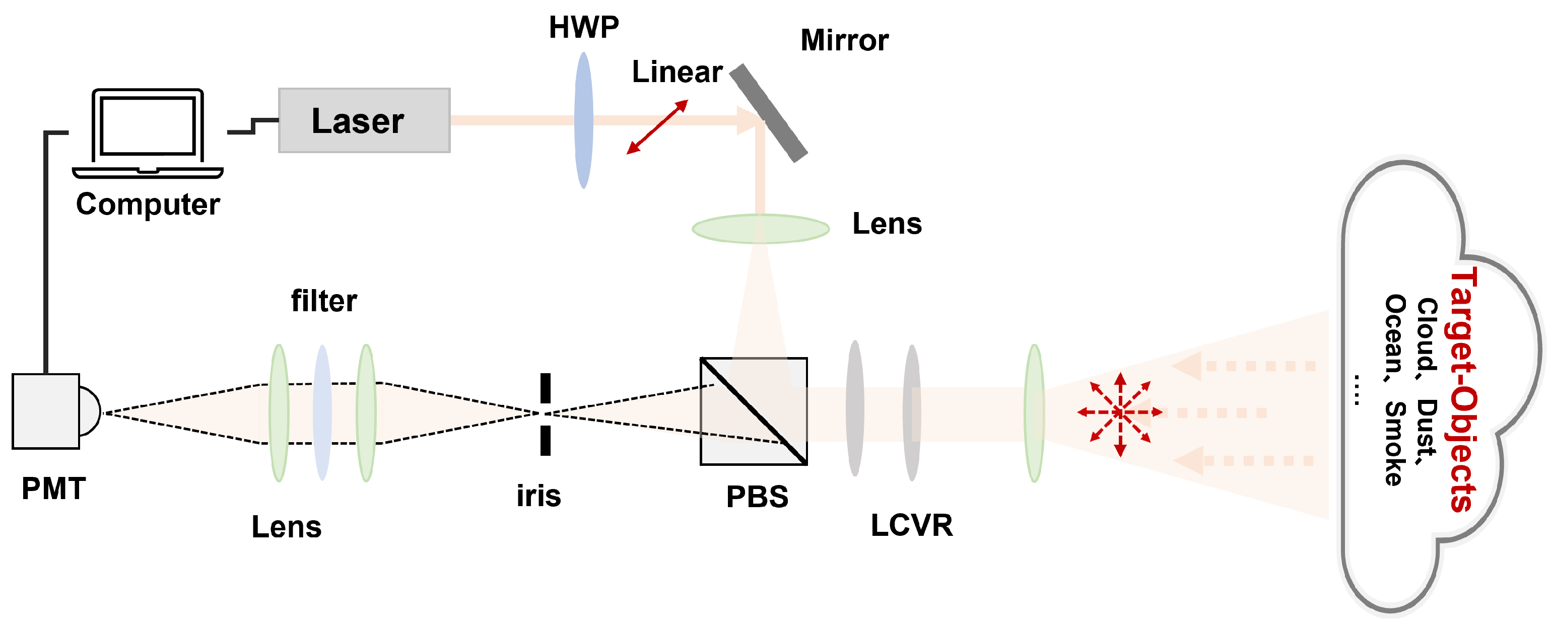
2.2.2. Single-Channel P-Lidar
2.2.3. Three/Four-Channel P-Lidar
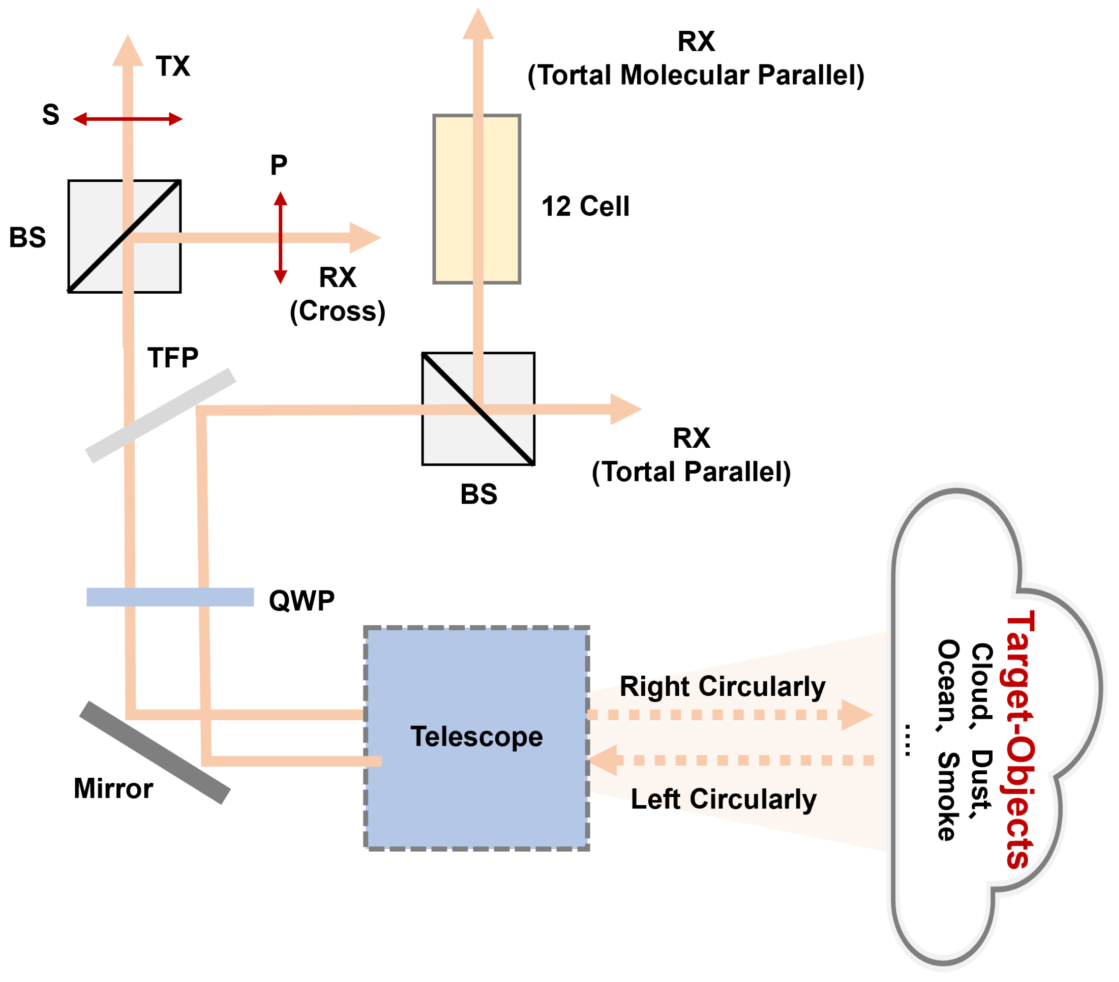
2.2.4. Full P-Lidar
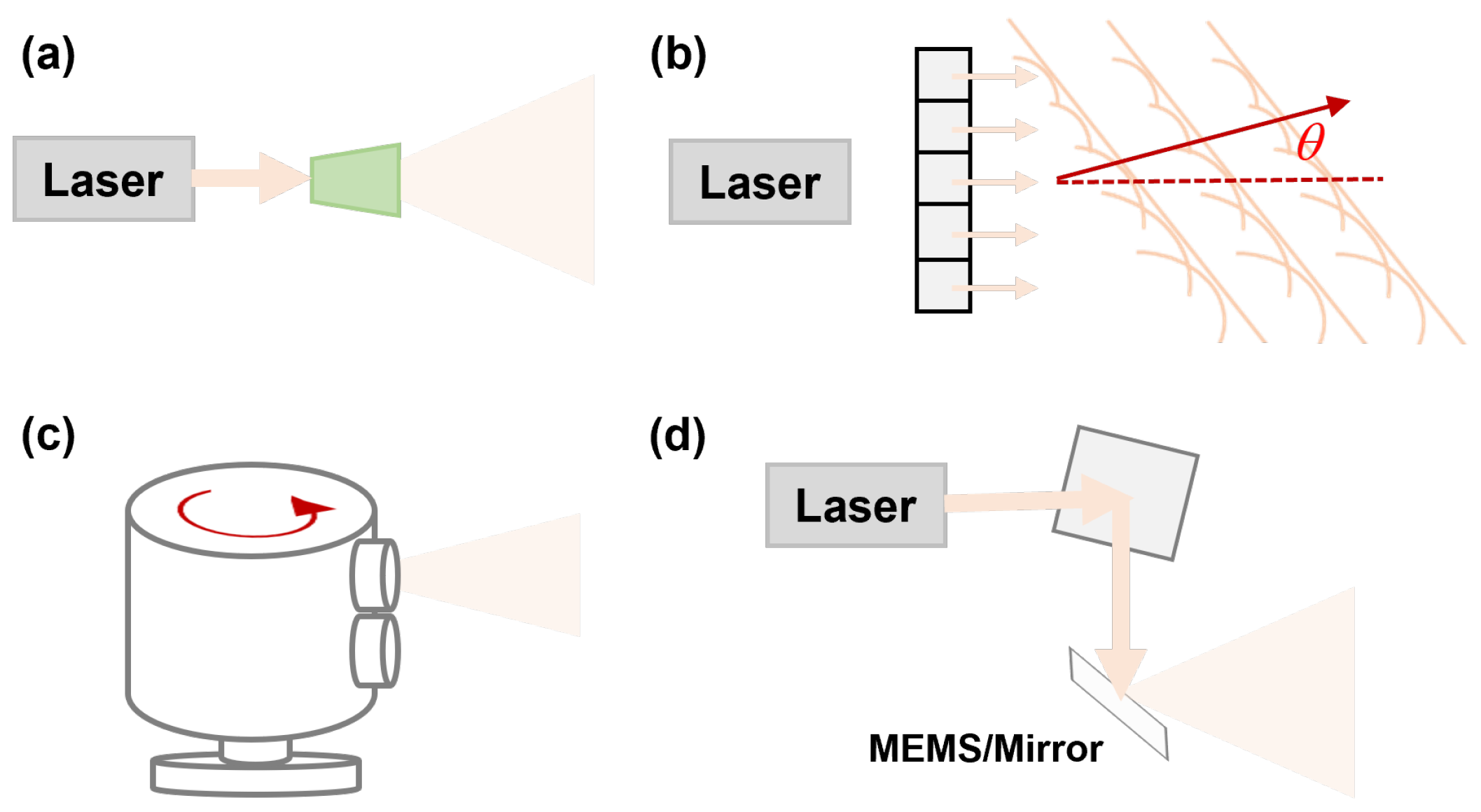
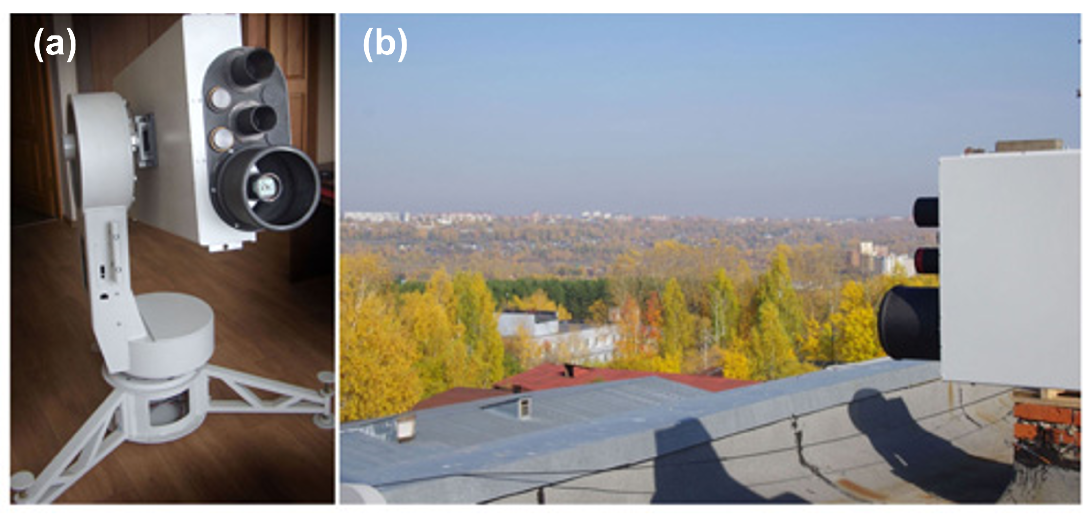
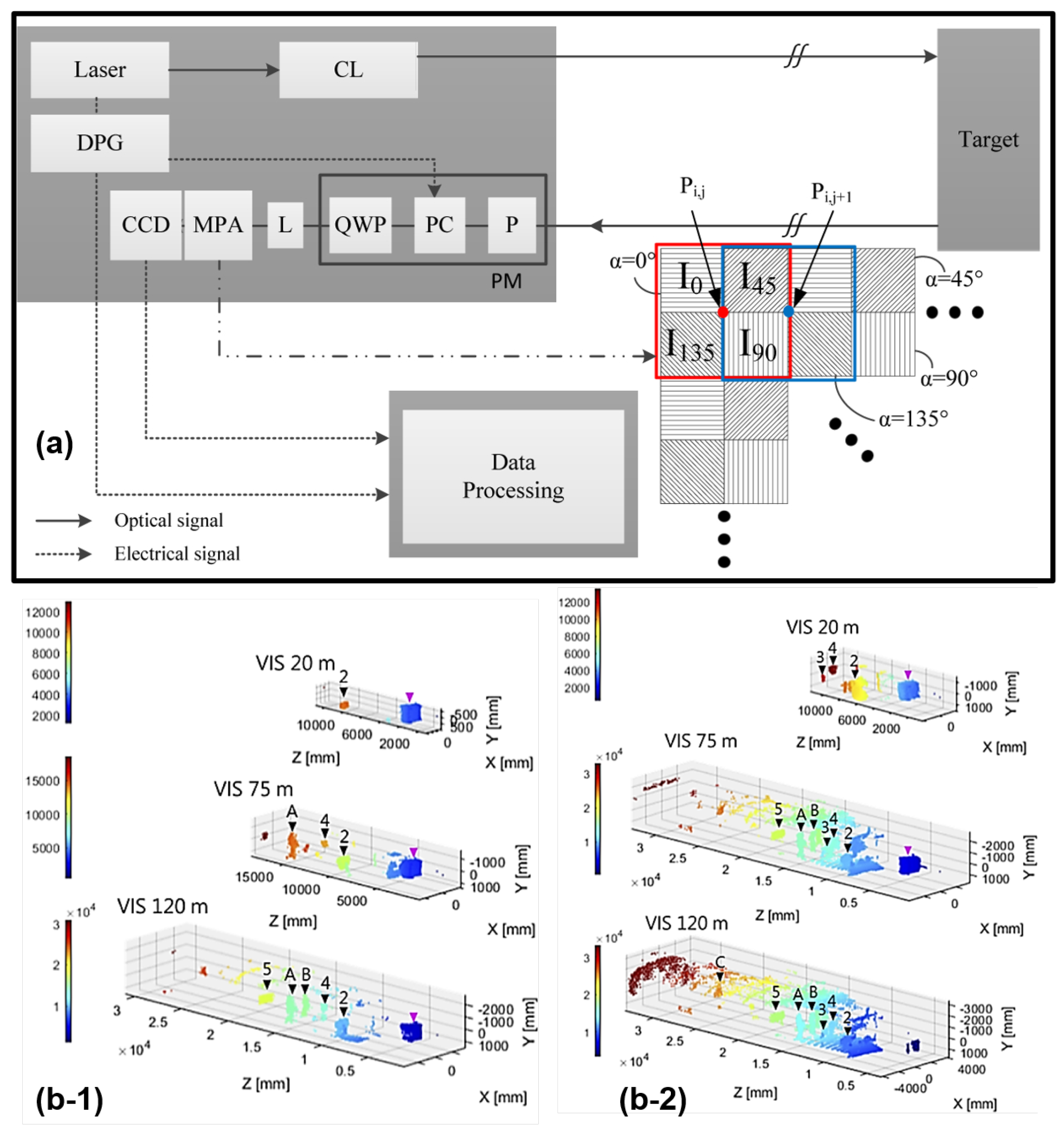
2.2.5. Scanning and Imaging P-Lidar Systems
2.2.6. Calibration for P-Lidar Systems
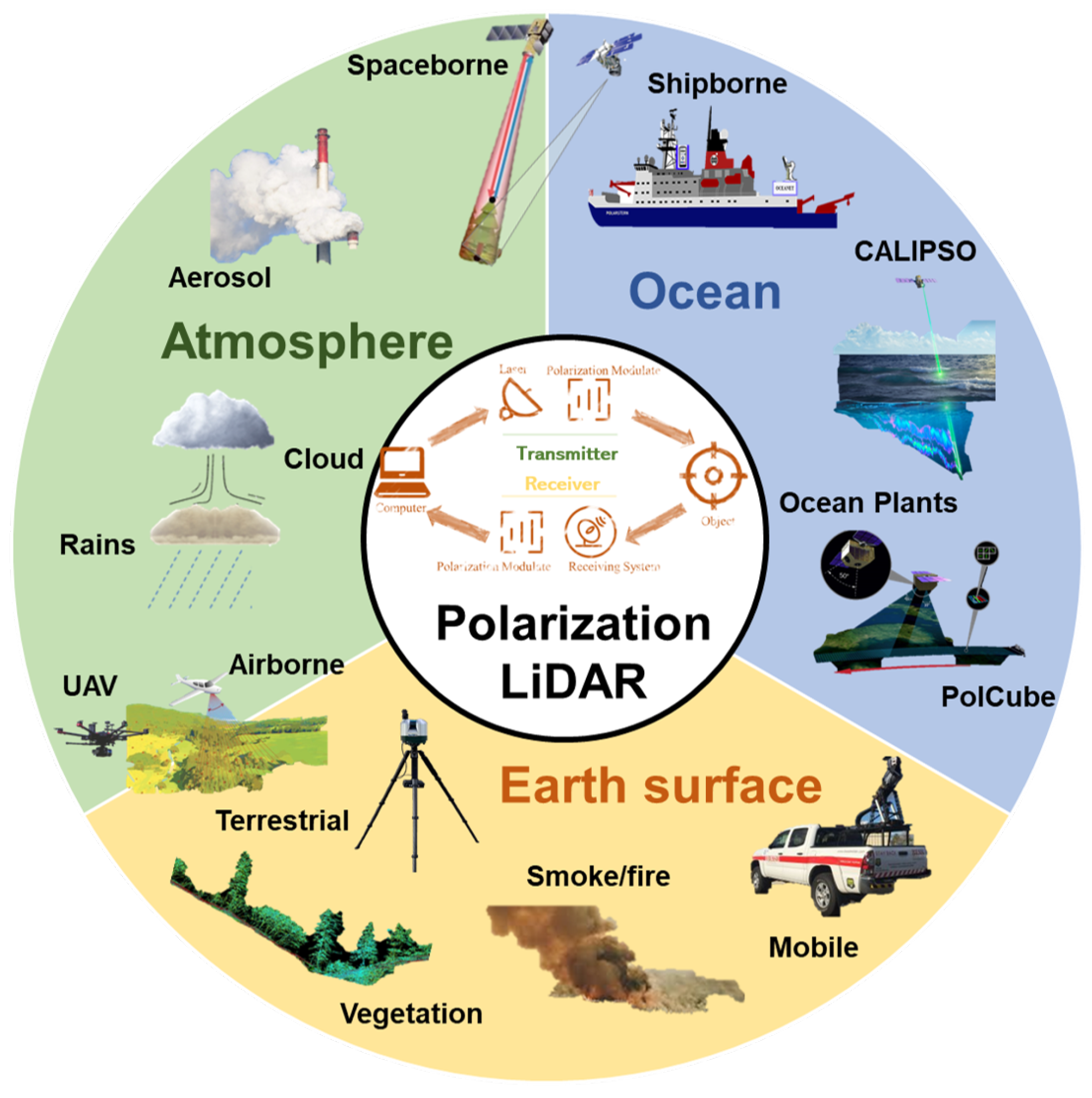
3. Applications
3.1. Atmospheric Remote Sensing
3.2. Remote Sensing of Earth’s Surface
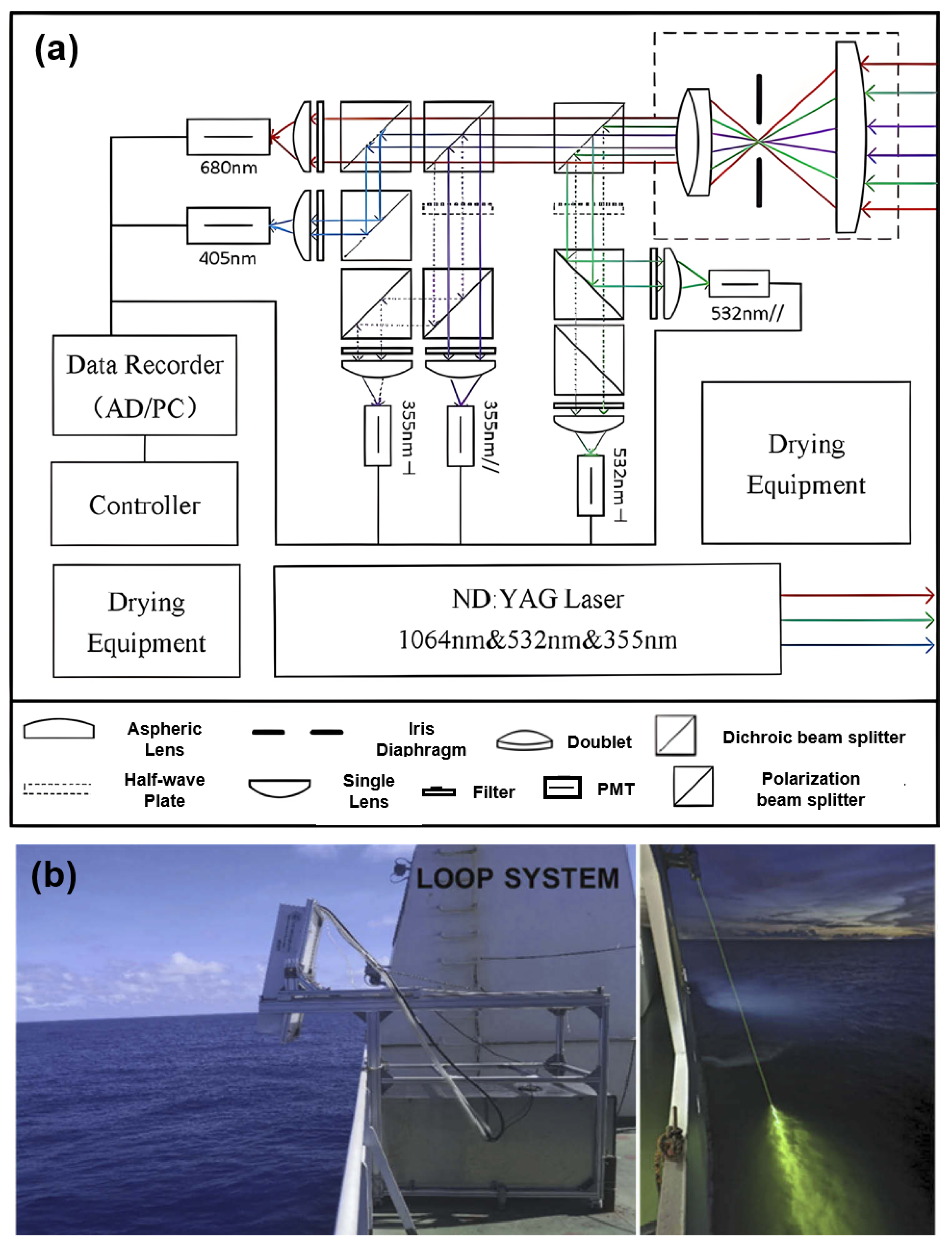
3.3. Ocean Remote Sensing
4. Conclusions
Author Contributions
Funding
Acknowledgments
Conflicts of Interest
Appendix A

| Abbreviation | Definition |
|---|---|
| 1C | Single-channel |
| 2C | Dual-channel |
| 4C | Four-channel |
| 3D | Three-dimensional |
| 2D | Two-dimensional |
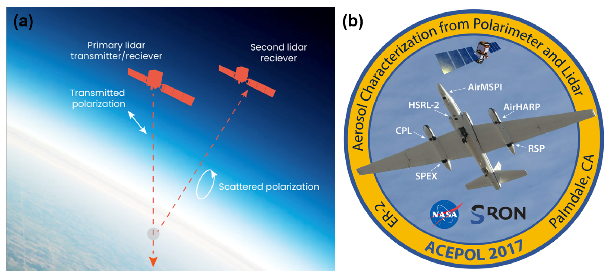
| ACEPOL | Aerosol Characterization from Polarimeter and Lidar |
| ACHSRL | Aerosol and Cloud High-Spectral-Resolution Lidar |
| ALPS | Airborne Laser Polarization Sensor |
| APD | Avalanche photodiode |
| ARM | Atmospheric radiation measurement |
| CALIOP | Cloud-Aerosol Lidar with Orthogonal Polarization |
| CAPABL | Clouds Aerosol Polarization and Backscatter Lidar |
| CCD | Charge-coupled device |
| CMOS | Complementary metal–oxide semiconductor |
| DNN | Deep neural network |
| DoFP | Division-of-focal-plane |
| DoLP | Degree of linear polarization |
| DoCP | Degree of circle polarization |
| EEL | Edge-emitting laser |
| EMCCD | Electron multiplying charge-coupled devices |
| FMCW | Frequency-modulated continuous wave |
| ER | Effective radius |
| ESA | European Space Agency |
| EUR | Europe |
| FOV | Field of view |
| FR | France |
| GR | Germany |
| HERA | Hybrid extinction retrieval algorithm |
| HSRL | High-spectral-resolution lidar |
| LASER | Light amplification by stimulated emissions of radiation |
| LED | Light-emitting diode |
| Lidar | Light detection and ranging |
| LOOP | Lidar for Ocean Optics Profiler |
| LSE | Light’s stimulated emission |
| MEMS | Micro-electro mechanical system |
| MiniSAR | Miniaturized synthetic aperture radar |
| MIT | Massachusetts Institute of Technology |
| MULIS | Multichannel Lidar System |
| NASA | National Aeronautics and Space Administration |
| Nd:YAG | Neodymium-doped yttrium aluminum garnet |
| NOAA | National Oceanic and Atmospheric Administration |
| OPA | Optical phased array |
| PBS | Polarization beam splitter |
| PD | Photodiode |
| P-Lidar | Polarization lidar |
| PMT | Photo-multiplier tube |
| POLIS | Portable lidar system |
| PSA | Polarization state analyzer |
| PSG | Polarization state generator |
| QWP | Quarter-wave plate |
| RT | Radiative transfer |
| SCA | Scene classification algorithms |
| SiPM | Silicon photo-multiplier |
| SIBYL | Selective Iterative Boundary Locator |
| SLICER | Scanning Lidar Imager of Canopies by Echo Recovery |
| SNR | Signal-to-noise ratio |
| SP | Single-photon |
| SPAD | Single-photon APD |
| SVLE | Stokes vector lidar |
| SWIR | Short-wave infrared |
| TOF | Time of flight |
| UAV | Unmanned aerial vehicles |
| USA | The United States of America |
| UV | Ultraviolet |
| VC | Volume concentration |
| VCSEL | Vertical-cavity surface-emitting laser |
| Vis–NIR | Visible, near-infrared |
| VLDR | Volume linear depolarization ratio |
| WACAL | Water vapor, cloud, and aerosol lidar |
References
- Pérez, J.J.G.; Ossikovski, R. Polarized Light and the Mueller Matrix Approach; CRC Press: Boca Raton, FL, USA, 2017. [Google Scholar]
- Goldstein, D.H. Polarized Light; CRC Press: Boca Raton, FL, USA, 2017. [Google Scholar]
- Bass, M.; Van Stryland, E.W.; Williams, D.R.; Wolfe, W.L. Handbook of Optics; McGraw-Hill: New York, NY, USA, 1995; Volume 2. [Google Scholar]
- Fowles, G.R. Introduction to Modern Optics; Courier Corporation: Washington, DC, USA, 1989. [Google Scholar]
- Li, X.; Hu, H.; Zhao, L.; Wang, H.; Yu, Y.; Wu, L.; Liu, T. Polarimetric image recovery method combining histogram stretching for underwater imaging. Sci. Rep. 2018, 8, 12430. [Google Scholar] [CrossRef] [PubMed]
- Li, X.; Han, Y.; Wang, H.; Liu, T.; Chen, S.C.; Hu, H. Polarimetric imaging through scattering media: A review. Front. Phys. 2022, 10, 815296. [Google Scholar] [CrossRef]
- Ballesta-Garcia, M.; Peña-Gutiérrez, S.; Rodríguez-Aramendía, A.; García-Gómez, P.; Rodrigo, N.; Bobi, A.R.; Royo, S. Analysis of the performance of a polarized LiDAR imager in fog. Opt. Express 2022, 30, 41524–41540. [Google Scholar] [CrossRef] [PubMed]
- Li, X.; Yan, L.; Qi, P.; Zhang, L.; Goudail, F.; Liu, T.; Zhai, J.; Hu, H. Polarimetric Imaging via Deep Learning: A Review. Remote Sens. 2023, 15, 1540. [Google Scholar] [CrossRef]
- Chu, J.; Zhao, K.; Zhang, Q.; Wang, T. Construction and performance test of a novel polarization sensor for navigation. Sens. Actuators Phys. 2008, 148, 75–82. [Google Scholar] [CrossRef]
- Wan, Z.; Zhao, K.; Chu, J. Robust azimuth measurement method based on polarimetric imaging for bionic polarization navigation. IEEE Trans. Instrum. Meas. 2019, 69, 5684–5692. [Google Scholar] [CrossRef]
- Sun, Z.; Zhang, J.; Zhao, Y. Laboratory studies of polarized light reflection from sea ice and lake ice in visible and near infrared. IEEE Geosci. Remote. Sens. Lett. 2012, 10, 170–173. [Google Scholar] [CrossRef]
- Sun, W.; Liu, Z.; Videen, G.; Fu, Q.; Muinonen, K.; Winker, D.M.; Lukashin, C.; Jin, Z.; Lin, B.; Huang, J. For the depolarization of linearly polarized light by smoke particles. J. Quant. Spectrosc. Radiat. Transf. 2013, 122, 233–237. [Google Scholar] [CrossRef]
- Kong, Z.; Ma, T.; Zheng, K.; Cheng, Y.; Gong, Z.; Hua, D.; Mei, L. Development of an all-day portable polarization Lidar system based on the division-of-focal-plane scheme for atmospheric polarization measurements. Opt. Express 2021, 29, 38512–38526. [Google Scholar] [CrossRef]
- Shibata, Y. Particle polarization Lidar for precipitation particle classification. Appl. Opt. 2022, 61, 1856–1862. [Google Scholar] [CrossRef]
- Sassen, K. The polarization Lidar technique for cloud research: A review and current assessment. Bull. Am. Meteorol. Soc. 1991, 72, 1848–1866. [Google Scholar] [CrossRef]
- Sassen, K. Polarization in Lidar. In LIDAR: Range-Resolved Optical Remote Sensing of the Atmosphere; Springer: Berlin/Heidelberg, Germany, 2005; pp. 19–42. [Google Scholar]
- Einstein, A. Näherungsweise integration der feldgleichungen der gravitation. Sitzungsberichte Königlich Preußischen Akad. Wiss. 1916, 22, 688–696. [Google Scholar]
- Herd, R.M.; Dover, J.S.; Arndt, K.A. Basic laser principles. Dermatol. Clin. 1997, 15, 355–372. [Google Scholar] [CrossRef]
- Zinth, W.; Laubereau, A.; Kaiser, W. The long journey to the laser and its rapid development after 1960. Eur. Phys. J. H 2011, 36, 153–181. [Google Scholar] [CrossRef]
- Collis, R. Lidar. Applied Optics 1970, 9, 1782–1788. [Google Scholar] [CrossRef]
- Dickey, J.O.; Bender, P.; Faller, J.; Newhall, X.; Ricklefs, R.; Ries, J.; Shelus, P.; Veillet, C.; Whipple, A.; Wiant, J.; et al. Lunar laser ranging: A continuing legacy of the Apollo program. Science 1994, 265, 482–490. [Google Scholar] [CrossRef]
- Bender, P.; Currie, D.; Poultney, S.; Alley, C.; Dicke, R.; Wilkinson, D.; Eckhardt, D.; Faller, J.; Kaula, W.; Mulholland, J.; et al. The Lunar Laser Ranging Experiment: Accurate ranges have given a large improvement in the lunar orbit and new selenophysical information. Science 1973, 182, 229–238. [Google Scholar] [CrossRef]
- Wandinger, U. Introduction to Lidar. In Lidar: Range-Resolved Optical Remote Sensing of the Atmosphere; Springer: Berlin/Heidelberg, Germany, 2005; pp. 1–18. [Google Scholar]
- Dubayah, R.O.; Drake, J.B. Lidar remote sensing for forestry. J. For. 2000, 98, 44–46. [Google Scholar]
- Dong, P.; Chen, Q. LiDAR Remote Sensing and Applications; CRC Press: Boca Raton, FL, USA, 2017. [Google Scholar]
- Han, Y.; Li, Z.; Wu, L.; Mai, S.; Xing, X.; Fu, H. High-Speed Two-Dimensional Spectral-Scanning Coherent LiDAR System Based on Tunable VCSEL. J. Light. Technol. 2022, 41, 412–419. [Google Scholar] [CrossRef]
- Sun, X.; Zhang, L.; Zhang, Q.; Zhang, W. Si photonics for practical LiDAR solutions. Appl. Sci. 2019, 9, 4225. [Google Scholar] [CrossRef]
- Shiina, T. LED mini Lidar for atmospheric application. Sensors 2019, 19, 569. [Google Scholar] [CrossRef] [PubMed]
- Sarbolandi, H.; Plack, M.; Kolb, A. Pulse based time-of-flight range sensing. Sensors 2018, 18, 1679. [Google Scholar] [CrossRef] [PubMed]
- Stove, A.G. Linear FMCW radar techniques. In IEE Proceedings F (Radar and Signal Processing); IET: Washington, DC, USA, 1992; Volume 139, pp. 343–350. [Google Scholar]
- McManamon, P.F.; Banks, P.; Beck, J.; Fried, D.G.; Huntington, A.S.; Watson, E.A. Comparison of flash Lidar detector options. Opt. Eng. 2017, 56, 031223. [Google Scholar] [CrossRef]
- Raj, T.; Hanim Hashim, F.; Baseri Huddin, A.; Ibrahim, M.F.; Hussain, A. A survey on LiDAR scanning mechanisms. Electronics 2020, 9, 741. [Google Scholar] [CrossRef]
- Tossoun, B.; Stephens, R.; Wang, Y.; Addamane, S.; Balakrishnan, G.; Holmes, A.; Beling, A. High-speed InP-based pin photodiodes with InGaAs/GaAsSb type-II quantum wells. IEEE Photonics Technol. Lett. 2018, 30, 399–402. [Google Scholar] [CrossRef]
- Villa, F.; Severini, F.; Madonini, F.; Zappa, F. SPADs and SiPMs arrays for long-range high-speed light detection and ranging (LiDAR). Sensors 2021, 21, 3839. [Google Scholar] [CrossRef]
- Beer, M.; Haase, J.F.; Ruskowski, J.; Kokozinski, R. Background light rejection in SPAD-based LiDAR sensors by adaptive photon coincidence detection. Sensors 2018, 18, 4338. [Google Scholar] [CrossRef] [PubMed]
- Behringer, M.; Johnson, K. Laser lightsources for LIDAR. In Proceedings of the 2021 27th International Semiconductor Laser Conference (ISLC), Potsdam, Germany, 10–14 October 2021; pp. 1–2. [Google Scholar]
- Wang, D.; Watkins, C.; Xie, H. MEMS mirrors for LiDAR: A review. Micromachines 2020, 11, 456. [Google Scholar] [CrossRef]
- Li, N.; Ho, C.P.; Xue, J.; Lim, L.W.; Chen, G.; Fu, Y.H.; Lee, L.Y.T. A progress review on solid-state LiDAR and nanophotonics-based LiDAR sensors. Laser Photonics Rev. 2022, 16, 2100511. [Google Scholar] [CrossRef]
- Schotland, R.M.; Sassen, K.; Stone, R. Observations by Lidar of linear depolarization ratios for hydrometeors. J. Appl. Meteorol. Climatol. 1971, 10, 1011–1017. [Google Scholar] [CrossRef]
- Platt, C.; Abshire, N.; McNice, G. Some microphysical properties of an ice cloud from Lidar observation of horizontally oriented crystals. J. Appl. Meteorol. Climatol. 1978, 17, 1220–1224. [Google Scholar] [CrossRef]
- Kalshoven, J.E.; Dabney, P.W. Remote sensing of the Earth’s surface with an airborne polarized laser. IEEE Trans. Geosci. Remote. Sens. 1993, 31, 438–446. [Google Scholar] [CrossRef]
- Churnside, J.H. Can we see fish from an airplane? In Airborne and In-Water Underwater Imaging; SPIE: Bellingham, WA, USA, 1999; Volume 3761, pp. 45–48. [Google Scholar]
- Kaul, B.V.; Samokhvalov, I.V.; Volkov, S.N. Investigating particle orientation in cirrus clouds by measuring backscattering phase matrices with Lidar. Appl. Opt. 2004, 43, 6620–6628. [Google Scholar] [CrossRef] [PubMed]
- Del Guasta, M.; Vallar, E.; Riviere, O.; Castagnoli, F.; Venturi, V.; Morandi, M. Use of polarimetric Lidar for the study of oriented ice plates in clouds. Appl. Opt. 2006, 45, 4878–4887. [Google Scholar] [CrossRef] [PubMed]
- Winker, D.; Hostetler, C.; Hunt, W. Caliop: The Calipso Lidar. In Proceedings of the 22nd Internation Laser Radar Conference (ILRC 2004), Matera, Italy, 12–16 July 2004; Volume 561, p. 941. [Google Scholar]
- Churnside, J.H.; Sharov, A.F.; Richter, R.A. Aerial surveys of fish in estuaries: A case study in Chesapeake Bay. ICES J. Mar. Sci. 2011, 68, 239–244. [Google Scholar] [CrossRef]
- Hayman, M.; Thayer, J.P. General description of polarization in Lidar using Stokes vectors and polar decomposition of Mueller matrices. JOSA A 2012, 29, 400–409. [Google Scholar] [CrossRef]
- Hayman, M.; Spuler, S.; Morley, B.; VanAndel, J. Polarization Lidar operation for measuring backscatter phase matrices of oriented scatterers. Opt. Express 2012, 20, 29553–29567. [Google Scholar] [CrossRef] [PubMed]
- Huang, Z.; Qi, S.; Zhou, T.; Dong, Q.; Ma, X.; Zhang, S.; Bi, J.; Shi, J. Investigation of aerosol absorption with dual-polarization Lidar observations. Opt. Express 2020, 28, 7028–7035. [Google Scholar] [CrossRef]
- Qiu, J.; Xia, H.; Shangguan, M.; Dou, X.; Li, M.; Wang, C.; Shang, X.; Lin, S.; Liu, J. Micro-pulse polarization Lidar at 1.5 μm using a single superconducting nanowire single-photon detector. Opt. Lett. 2017, 42, 4454–4457. [Google Scholar] [CrossRef]
- Stillwell, R.A.; Neely, R.R., III; Thayer, J.P.; Shupe, M.D.; Turner, D.D. Improved cloud-phase determination of low-level liquid and mixed-phase clouds by enhanced polarimetric Lidar. Atmos. Meas. Tech. 2018, 11, 835–859. [Google Scholar] [CrossRef]
- Kokhanenko, G.P.; Balin, Y.S.; Klemasheva, M.G.; Nasonov, S.V.; Novoselov, M.M.; Penner, I.E.; Samoilova, S.V. Scanning polarization Lidar LOSA-M3: Opportunity for research of crystalline particle orientation in the ice clouds. Atmos. Meas. Tech. 2020, 13, 1113–1127. [Google Scholar] [CrossRef]
- Qi, S.; Huang, Z.; Ma, X.; Huang, J.; Zhou, T.; Zhang, S.; Dong, Q.; Bi, J.; Shi, J. Classification of atmospheric aerosols and clouds by use of dual-polarization Lidar measurements. Opt. Express 2021, 29, 23461–23476. [Google Scholar] [CrossRef]
- Kong, Z.; Ma, T.; Cheng, Y.; Fei, R.; Zhang, Z.; Li, Y.; Mei, L. A polarization-sensitive imaging Lidar for atmospheric remote sensing. J. Quant. Spectrosc. Radiat. Transf. 2021, 271, 107747. [Google Scholar] [CrossRef]
- Kong, Z.; Yu, J.; Gong, Z.; Hua, D.; Mei, L. Visible, near-infrared dual-polarization Lidar based on polarization cameras: System design, evaluation and atmospheric measurements. Opt. Express 2022, 30, 28514–28533. [Google Scholar] [CrossRef]
- Hulst, H.C.; van de Hulst, H.C. Light Scattering by Small Particles; Courier Corporation: Washington, DC, USA, 1981. [Google Scholar]
- Chen, W.; Zheng, Q.; Xiang, H.; Chen, X.; Sakai, T. Forest canopy height estimation using polarimetric interferometric synthetic aperture radar (PolInSAR) technology based on full-polarized ALOS/PALSAR data. Remote Sens. 2021, 13, 174. [Google Scholar] [CrossRef]
- Buurman, P.; Pape, T.; Muggler, C. Laser grain-size determination in soil genetic studies 1. Practical problems. Soil Sci. 1997, 162, 211–218. [Google Scholar] [CrossRef]
- Sassen, K.; Zhu, J.; Webley, P.; Dean, K.; Cobb, P. Volcanic ash plume identification using polarization Lidar: Augustine eruption, Alaska. Geophys. Res. Lett. 2007, 34. [Google Scholar] [CrossRef]
- David, G.; Thomas, B.; Nousiainen, T.; Miffre, A.; Rairoux, P. Retrieving simulated volcanic, desert dust and sea-salt particle properties from two/three-component particle mixtures using UV-VIS polarization Lidar and T matrix. Atmos. Chem. Phys. 2013, 13, 6757–6776. [Google Scholar] [CrossRef]
- Pal, S.; Carswell, A. The polarization characteristics of Lidar scattering from snow and ice crystals in the atmosphere. J. Appl. Meteorol. Climatol. 1977, 16, 70–80. [Google Scholar] [CrossRef]
- Gibbs, D.P.; Betty, C.L.; Bredow, J.W.; Fung, A.K. Polarized and cross-polarized angular reflectance characteristics of saline ice and snow. Remote Sens. Rev. 1993, 7, 179–195. [Google Scholar] [CrossRef]
- Liu, Q.; Wu, S.; Liu, B.; Liu, J.; Zhang, K.; Dai, G.; Tang, J.; Chen, G. Shipborne variable-FOV, dual-wavelength, polarized ocean Lidar: Design and measurements in the Western Pacific. Opt. Express 2022, 30, 8927–8948. [Google Scholar] [CrossRef] [PubMed]
- Behrenfeld, M.J.; Hu, Y.; O’Malley, R.T.; Boss, E.S.; Hostetler, C.A.; Siegel, D.A.; Sarmiento, J.L.; Schulien, J.; Hair, J.W.; Lu, X.; et al. Annual boom–bust cycles of polar phytoplankton biomass revealed by space-based Lidar. Nat. Geosci. 2017, 10, 118–122. [Google Scholar] [CrossRef]
- Behrenfeld, M.J.; Gaube, P.; Della Penna, A.; O’malley, R.T.; Burt, W.J.; Hu, Y.; Bontempi, P.S.; Steinberg, D.K.; Boss, E.S.; Siegel, D.A.; et al. Global satellite-observed daily vertical migrations of ocean animals. Nature 2019, 576, 257–261. [Google Scholar] [CrossRef] [PubMed]
- Hoge, F.E.; Wright, C.W.; Krabill, W.B.; Buntzen, R.R.; Gilbert, G.D.; Swift, R.N.; Yungel, J.K.; Berry, R.E. Airborne Lidar detection of subsurface oceanic scattering layers. Appl. Opt. 1988, 27, 3969–3977. [Google Scholar] [CrossRef] [PubMed]
- Churnside, J.H. Polarization effects on oceanographic Lidar. Opt. Express 2008, 16, 1196–1207. [Google Scholar] [CrossRef] [PubMed]
- Churnside, J.H.; Sullivan, J.M.; Twardowski, M.S. Lidar extinction-to-backscatter ratio of the ocean. Opt. Express 2014, 22, 18698–18706. [Google Scholar] [CrossRef] [PubMed]
- Churnside, J.H.; Marchbanks, R.D. Inversion of oceanographic profiling Lidars by a perturbation to a linear regression. Appl. Opt. 2017, 56, 5228–5233. [Google Scholar] [CrossRef]
- Chen, P.; Jamet, C.; Zhang, Z.; He, Y.; Mao, Z.; Pan, D.; Wang, T.; Liu, D.; Yuan, D. Vertical distribution of subsurface phytoplankton layer in South China Sea using airborne Lidar. Remote Sens. Environ. 2021, 263, 112567. [Google Scholar] [CrossRef]
- Dassot, M.; Constant, T.; Fournier, M. The use of terrestrial LiDAR technology in forest science: Application fields, benefits and challenges. Ann. For. Sci. 2011, 68, 959–974. [Google Scholar] [CrossRef]
- Kemeny, J.; Turner, K. Ground-Based Lidar: Rock Slope Mapping and Assessment; Technical report; Federal Highway Administration, Central Federal Lands Highway Division: Washington, DC, USA, 2008.
- Williams, K.; Olsen, M.J.; Roe, G.V.; Glennie, C. Synthesis of transportation applications of mobile LiDAR. Remote Sens. 2013, 5, 4652–4692. [Google Scholar] [CrossRef]
- Ecke, S.; Dempewolf, J.; Frey, J.; Schwaller, A.; Endres, E.; Klemmt, H.J.; Tiede, D.; Seifert, T. UAV-based forest health monitoring: A systematic review. Remote Sens. 2022, 14, 3205. [Google Scholar] [CrossRef]
- Vasilkov, A.P.; Goldin, Y.A.; Gureev, B.A.; Hoge, F.E.; Swift, R.N.; Wright, C.W. Airborne polarized Lidar detection of scattering layers in the ocean. Appl. Opt. 2001, 40, 4353–4364. [Google Scholar] [CrossRef] [PubMed]
- Goldin, Y.A.; Gureev, B.A.; Ventskut, Y.I. Shipboard polarized Lidar for seawater column sounding. In Current Research on Remote Sensing, Laser Probing, and Imagery in Natural Waters; SPIE: Bellingham, WA, USA, 2007; Volume 6615, pp. 152–159. [Google Scholar]
- Okamoto, H.; Sato, K.; Borovoi, A.; Ishimoto, H.; Masuda, K.; Konoshonkin, A.; Kustova, N. Interpretation of Lidar ratio and depolarization ratio of ice clouds using spaceborne high-spectral-resolution polarization Lidar. Opt. Express 2019, 27, 36587–36600. [Google Scholar] [CrossRef] [PubMed]
- Li, X.; Liu, T.; Huang, B.; Song, Z.; Hu, H. Optimal distribution of integration time for intensity measurements in Stokes polarimetry. Opt. Express 2015, 23, 27690–27699. [Google Scholar] [CrossRef] [PubMed]
- Li, X.; Hu, H.; Wu, L.; Liu, T. Optimization of instrument matrix for Mueller matrix ellipsometry based on partial elements analysis of the Mueller matrix. Opt. Express 2017, 25, 18872–18884. [Google Scholar] [CrossRef] [PubMed]
- Stokes, G.G. On the composition and resolution of streams of polarized light from different sources. Trans. Camb. Philos. Soc. 1851, 9, 399. [Google Scholar]
- Li, X.; Hu, H.; Liu, T.; Huang, B.; Song, Z. Optimal distribution of integration time for intensity measurements in degree of linear polarization polarimetry. Opt. Express 2016, 24, 7191–7200. [Google Scholar] [CrossRef] [PubMed]
- Song, Z.; Li, X.; Liu, T. Optimal distribution of integration time in degree of linear polarization polarimetry based on the expected variance. Optik 2017, 136, 123–128. [Google Scholar] [CrossRef]
- Chen, W.N.; Chiang, C.W.; Nee, J.B. Lidar ratio and depolarization ratio for cirrus clouds. Appl. Opt. 2002, 41, 6470–6476. [Google Scholar] [CrossRef]
- Noel, V.; Chepfer, H.; Ledanois, G.; Delaval, A.; Flamant, P.H. Classification of particle effective shape ratios in cirrus clouds based on the Lidar depolarization ratio. Appl. Opt. 2002, 41, 4245–4257. [Google Scholar] [CrossRef]
- Lu, S.Y.; Chipman, R.A. Interpretation of Mueller matrices based on polar decomposition. JOSA A 1996, 13, 1106–1113. [Google Scholar] [CrossRef]
- Morio, J.; Goudail, F. Influence of the order of diattenuator, retarder, and polarizer in polar decomposition of Mueller matrices. Opt. Lett. 2004, 29, 2234–2236. [Google Scholar] [CrossRef] [PubMed]
- Gil, J.J.; San José, I.; Ossikovski, R. Serial–parallel decompositions of Mueller matrices. JOSA A 2013, 30, 32–50. [Google Scholar] [CrossRef] [PubMed]
- Li, X.; Zhang, L.; Qi, P.; Zhu, Z.; Xu, J.; Liu, T.; Zhai, J.; Hu, H. Are indices of polarimetric purity excellent metrics for object identification in scattering media? Remote Sens. 2022, 14, 4148. [Google Scholar] [CrossRef]
- Li, X.; Liu, W.; Goudail, F.; Chen, S.C. Optimal nonlinear Stokes—Mueller polarimetry for multi-photon processes. Opt. Lett. 2022, 47, 3287–3290. [Google Scholar] [CrossRef] [PubMed]
- Li, X.; Goudail, F.; Chen, S.C. Self-calibration for Mueller polarimeters based on DoFP polarization imagers. Opt. Lett. 2022, 47, 1415–1418. [Google Scholar] [CrossRef] [PubMed]
- Chandrasekar, V.; Keränen, R.; Lim, S.; Moisseev, D. Recent advances in classification of observations from dual polarization weather radars. Atmos. Res. 2013, 119, 97–111. [Google Scholar] [CrossRef]
- Sassen, K.; Wang, Z.; Liu, D. Global distribution of cirrus clouds from CloudSat/Cloud-Aerosol Lidar and infrared pathfinder satellite observations (CALIPSO) measurements. J. Geophys. Res. Atmos. 2008, 113, D8. [Google Scholar] [CrossRef]
- Ahmad, W.; Zhang, K.; Tong, Y.; Xiao, D.; Wu, L.; Liu, D. Water cloud detection with circular polarization Lidar: A semianalytic Monte Carlo simulation approach. Sensors 2022, 22, 1679. [Google Scholar] [CrossRef]
- Evans, B.T.N. On the Inversion of the Lidar Equation; Department of National Defence, Research and Development Branch, Defence Research Establishment: Umea, Sweden, 1984. [Google Scholar]
- Northend, C.; Honey, R.; Evans, W. Laser radar (Lidar) for meteorological observations. Rev. Sci. Instrum. 1966, 37, 393–400. [Google Scholar] [CrossRef]
- Sasano, Y.; Shimizu, H.; Takeuchi, N.; Okuda, M. Geometrical form factor in the laser radar equation: An experimental determination. Appl. Opt. 1979, 18, 3908–3910. [Google Scholar] [CrossRef] [PubMed]
- Biele, J.; Beyerle, G.; Baumgarten, G. Polarization Lidar: Corrections of instrumental effects. Opt. Express 2000, 7, 427–435. [Google Scholar] [CrossRef] [PubMed]
- Freudenthaler, V. About the effects of polarising optics on Lidar signals and the Δ90 calibration. Atmos. Meas. Tech. 2016, 9, 4181–4255. [Google Scholar] [CrossRef]
- Winker, D.M.; Vaughan, M.A.; Omar, A.; Hu, Y.; Powell, K.A.; Liu, Z.; Hunt, W.H.; Young, S.A. Overview of the CALIPSO mission and CALIOP data processing algorithms. J. Atmos. Ocean. Technol. 2009, 26, 2310–2323. [Google Scholar] [CrossRef]
- Winker, D.M.; Hunt, W.H.; McGill, M.J. Initial performance assessment of CALIOP. Geophys. Res. Lett. 2007, 34, 19. [Google Scholar] [CrossRef]
- Winker, D.; Pelon, J.; Coakley, J., Jr.; Ackerman, S.; Charlson, R.; Colarco, P.; Flamant, P.; Fu, Q.; Hoff, R.; Kittaka, C.; et al. The CALIPSO mission: A global 3D view of aerosols and clouds. Bull. Am. Meteorol. Soc. 2010, 91, 1211–1230. [Google Scholar] [CrossRef]
- Sarabandi, K.; Ulaby, F.T.; Tassoudji, M.A. Calibration of polarimetric radar systems with good polarization isolation. IEEE Trans. Geosci. Remote Sens. 1990, 28, 70–75. [Google Scholar] [CrossRef]
- Alvarez, J.; Vaughan, M.A.; Hostetler, C.A.; Hunt, W.; Winker, D.M. Calibration technique for polarization-sensitive Lidars. J. Atmos. Ocean. Technol. 2006, 23, 683–699. [Google Scholar] [CrossRef]
- Platt, C. Lidar observation of a mixed-phase altostratus cloud. J. Appl. Meteorol. Climatol. 1977, 16, 339–345. [Google Scholar] [CrossRef]
- Flynna, C.J.; Mendozaa, A.; Zhengb, Y.; Mathurb, S. Novel polarization-sensitive micropulse Lidar measurement technique. Opt. Express 2007, 15, 2785–2790. [Google Scholar] [CrossRef]
- Pal, S.; Carswell, A. Polarization properties of Lidar backscattering from clouds. Appl. Opt. 1973, 12, 1530–1535. [Google Scholar] [CrossRef] [PubMed]
- Houston, J.; Carswell, A. Four-component polarization measurement of Lidar atmospheric scattering. Appl. Opt. 1978, 17, 614–620. [Google Scholar] [CrossRef] [PubMed]
- Xian, J.; Xu, W.; Long, C.; Song, Q.; Yang, S. Early forest-fire detection using scanning polarization Lidar. Appl. Opt. 2020, 59, 8638–8644. [Google Scholar] [CrossRef] [PubMed]
- Noel, V.; Sassen, K. Study of planar ice crystal orientations in ice clouds from scanning polarization Lidar observations. J. Appl. Meteorol. Climatol. 2005, 44, 653–664. [Google Scholar] [CrossRef]
- Sassen, K. Polarization in Lidar: A review. Polariz. Sci. Remote Sens. 2003, 5158, 151–160. [Google Scholar]
- Li, C.; Xu, S.; Zhao, L.; Cheng, G. Research on MEMS biaxial electromagnetic micromirror based on radial magnetic field distribution. In Proceedings of the International Conference on Laser, Optics and Optoelectronic Technology (LOPET 2021), Xi’an, China, 28–30 May 2021; Volume 11885, pp. 206–212. [Google Scholar]
- Roriz, R.; Cabral, J.; Gomes, T. Automotive LiDAR technology: A survey. IEEE Trans. Intell. Transp. Syst. 2021, 23, 6282–6297. [Google Scholar] [CrossRef]
- Kokhanenko, G.P. Possibilities of using mirror scanners in polarizing Lidars. In Proceedings of the 28th International Symposium on Atmospheric and Ocean Optics: Atmospheric Physics, Tomsk, Russia, 4–8 July 2022; Volume 12341, pp. 328–333. [Google Scholar]
- Li, X.; Li, Y.; Xie, X.; Xu, L. Laser polarization imaging models based on leaf moisture content. Infrared Laser Eng. 2017, 46, 1106004. (In Chinese) [Google Scholar]
- Behrendt, A.; Nakamura, T. Calculation of the calibration constant of polarization Lidar and its dependency on atmospheric temperature. Opt. Express 2002, 10, 805–817. [Google Scholar] [CrossRef]
- Luo, J.; Liu, D.; Bi, L.; Zhang, K.; Tang, P.; Xu, P.; Su, L.; Yang, L. Rotating a half-wave plate by 45: An ideal calibration method for the gain ratio in polarization Lidars. Opt. Commun. 2018, 407, 361–366. [Google Scholar] [CrossRef]
- Mattis, I.; Tesche, M.; Grein, M.; Freudenthaler, V.; Müller, D. Systematic error of Lidar profiles caused by a polarization-dependent receiver transmission: Quantification and error correction scheme. Appl. Opt. 2009, 48, 2742–2751. [Google Scholar] [CrossRef]
- Hunt, W.H.; Winker, D.M.; Vaughan, M.A.; Powell, K.A.; Lucker, P.L.; Weimer, C. CALIPSO Lidar description and performance assessment. J. Atmos. Ocean. Technol. 2009, 26, 1214–1228. [Google Scholar] [CrossRef]
- Sassen, K.; Benson, S. A midlatitude cirrus cloud climatology from the Facility for Atmospheric Remote Sensing. Part II: Microphysical properties derived from Lidar depolarization. J. Atmos. Sci. 2001, 58, 2103–2112. [Google Scholar] [CrossRef]
- Tong, Y.; Tong, X.; Zhang, K.; Xiao, D.; Rong, Y.; Zhou, Y.; Liu, C.; Liu, D. Polarization Lidar gain ratio calibration method: A comparison. Chin. Opt. 2021, 14, 685–703. [Google Scholar]
- Luo, J.; Liu, D.; Huang, Z.; Wang, B.; Bai, J.; Cheng, Z.; Zhang, Y.; Tang, P.; Yang, L.; Su, L. Polarization properties of receiving telescopes in atmospheric remote sensing polarization Lidars. Appl. Opt. 2017, 56, 6837–6845. [Google Scholar] [CrossRef] [PubMed]
- Freudenthaler, V.; Esselborn, M.; Wiegner, M.; Heese, B.; Tesche, M.; Ansmann, A.; Müller, D.; Althausen, D.; Wirth, M.; Fix, A.; et al. Depolarization ratio profiling at several wavelengths in pure Saharan dust during SAMUM 2006. Tellus Chem. Phys. Meteorol. 2009, 61, 165–179. [Google Scholar] [CrossRef]
- Fiocco, G.; Smullin, L. Detection of scattering layers in the upper atmosphere (60–140 km) by optical radar. Nature 1963, 199, 1275–1276. [Google Scholar] [CrossRef]
- Polarization Lidar. Available online: https://www.tropos.de/en/research/projects-infrastructures-technology/technology-at-tropos/remote-sensing/polarization-Lidar (accessed on 3 September 2023).
- Matrosov, S.Y.; Schmitt, C.G.; Maahn, M.; de Boer, G. Atmospheric ice particle shape estimates from polarimetric radar measurements and in situ observations. J. Atmos. Ocean. Technol. 2017, 34, 2569–2587. [Google Scholar] [CrossRef]
- Wu, S.; Song, X.; Liu, B.; Dai, G.; Liu, J.; Zhang, K.; Qin, S.; Hua, D.; Gao, F.; Liu, L. Mobile multi-wavelength polarization Raman Lidar for water vapor, cloud and aerosol measurement. Opt. Express 2015, 23, 33870–33892. [Google Scholar] [CrossRef]
- Tan, W.; Li, C.; Liu, Y.; Meng, X.; Wu, Z.; Kang, L.; Zhu, T. Potential of polarization Lidar to profile the urban aerosol phase state during haze episodes. Environ. Sci. Technol. Lett. 2019, 7, 54–59. [Google Scholar] [CrossRef]
- Jimenez, C.; Ansmann, A.; Engelmann, R.; Donovan, D.; Malinka, A.; Jörg, S.; Patric, S.; Ulla, W. The dual-field-of-view polarization Lidar technique: A new concept in monitoring aerosol effects in liquid-water clouds—Theoretical framework. Atmos. Chem. Phys. 2020, 20, 15247–15263. [Google Scholar] [CrossRef]
- Jimenez, C.; Ansmann, A.; Engelmann, R.; Donovan, D.; Malinka, A.; Seifert, P.; Wiesen, R.; Radenz, M.; Yin, Z.; Bühl, J.; et al. The dual-field-of-view polarization Lidar technique: A new concept in monitoring aerosol effects in liquid-water clouds—Case studies. Atmos. Chem. Phys. 2020, 20, 15265–15284. [Google Scholar] [CrossRef]
- Zhang, S.; Huang, Z.; Alam, K.; Li, M.; Dong, Q.; Wang, Y.; Shen, X.; Bi, J.; Zhang, J.; Li, W.; et al. Derived Profiles of CCN and INP Number Concentrations in the Taklimakan Desert via Combined Polarization Lidar, Sun-Photometer, and Radiosonde Observations. Remote Sens. 2023, 15, 1216. [Google Scholar] [CrossRef]
- Pal, S.; Carswell, A. Polarization properties of Lidar scattering from clouds at 347 nm and 694 nm. Appl. Opt. 1978, 17, 2321–2328. [Google Scholar] [CrossRef] [PubMed]
- Sassen, K.; Zhao, H.; Dodd, G.C. Simulated polarization diversity Lidar returns from water and precipitating mixed phase clouds. Appl. Opt. 1992, 31, 2914–2923. [Google Scholar] [CrossRef]
- Mamouri, R.E.; Ansmann, A. Potential of polarization Lidar to provide profiles of CCN-and INP-relevant aerosol parameters. Atmos. Chem. Phys. 2016, 16, 5905–5931. [Google Scholar] [CrossRef]
- Ansmann, A.; Ohneiser, K.; Mamouri, R.E.; Knopf, D.A.; Veselovskii, I.; Baars, H.; Engelmann, R.; Foth, A.; Jimenez, C.; Seifert, P.; et al. Tropospheric and stratospheric wildfire smoke profiling with Lidar: Mass, surface area, CCN, and INP retrieval. Atmos. Chem. Phys. 2021, 21, 9779–9807. [Google Scholar] [CrossRef]
- Murayama, T.; Müller, D.; Wada, K.; Shimizu, A.; Sekiguchi, M.; Tsukamoto, T. Characterization of Asian dust and Siberian smoke with multi-wavelength Raman Lidar over Tokyo, Japan in spring 2003. Geophys. Res. Lett. 2004, 31, 23. [Google Scholar] [CrossRef]
- Sugimoto, N.; Lee, C.H. Characteristics of dust aerosols inferred from Lidar depolarization measurements at two wavelengths. Appl. Opt. 2006, 45, 7468–7474. [Google Scholar] [CrossRef]
- Sugimoto, N.; Uno, I.; Nishikawa, M.; Shimizu, A.; Matsui, I.; Dong, X.; Chen, Y.; Quan, H. Record heavy Asian dust in Beijing in 2002: Observations and model analysis of recent events. Geophys. Res. Lett. 2003, 30, 12. [Google Scholar] [CrossRef]
- Tesche, M.; Ansmann, A.; Müller, D.; Althausen, D.; Engelmann, R.; Freudenthaler, V.; Groß, S. Vertically resolved separation of dust and smoke over Cape Verde using multiwavelength Raman and polarization Lidars during Saharan Mineral Dust Experiment 2008. J. Geophys. Res. Atmos. 2009, 114, D13. [Google Scholar] [CrossRef]
- Burton, S.; Hair, J.; Kahnert, M.; Ferrare, R.; Hostetler, C.; Cook, A.; Harper, D.; Berkoff, T.; Seaman, S.; Collins, J.; et al. Observations of the spectral dependence of linear particle depolarization ratio of aerosols using NASA Langley airborne High Spectral Resolution Lidar. Atmos. Chem. Phys. 2015, 15, 13453–13473. [Google Scholar] [CrossRef]
- Haarig, M.; Althausen, D.; Ansmann, A.; Klepel, A.; Baars, H.; Engelmann, R.; Groß, S.; Freudenthaler, V. Measurement of the linear depolarization ratio of aged dust at three wavelengths (355, 532 and 1064 nm) simultaneously over Barbados. In EPJ Web of Conferences; EDP Sciences: Les Ulis, France, 2016; Volume 119, p. 18009. [Google Scholar]
- Vaughan, M.; Garnier, A.; Josset, D.; Avery, M.; Lee, K.P.; Liu, Z.; Hunt, W.; Pelon, J.; Hu, Y.; Burton, S.; et al. CALIPSO Lidar calibration at 1064 nm: Version 4 algorithm. Atmos. Meas. Tech. 2019, 12, 51–82. [Google Scholar] [CrossRef]
- Tsekeri, A.; Amiridis, V.; Louridas, A.; Georgoussis, G.; Freudenthaler, V.; Metallinos, S.; Doxastakis, G.; Gasteiger, J.; Siomos, N.; Paschou, P.; et al. Polarization Lidar for detecting dust orientation: System design and calibration. Atmos. Meas. Tech. 2021, 14, 7453–7474. [Google Scholar] [CrossRef]
- Seckar, C.; Guy, L.; DiFronzo, A.; Weimer, C. Performance testing of an active boresight mechanism for use in the CALIPSO space bourne LIDAR mission. In Optomechanics 2005; SPIE: Bellingham, WA, USA, 2005; Volume 5877, pp. 319–330. [Google Scholar]
- Atmospheric Aerosol Characterization. Available online: https://www.ll.mit.edu/r-d/projects/atmospheric-aerosol-characterization (accessed on 3 September 2023).
- Knobelspiesse, K.; Barbosa, H.M.; Bradley, C.; Bruegge, C.; Cairns, B.; Chen, G.; Chowdhary, J.; Cook, A.; Di Noia, A.; van Diedenhoven, B.; et al. The Aerosol Characterization from Polarimeter and Lidar (ACEPOL) airborne field campaign. Earth Syst. Sci. Data Discuss. 2020, 2020, 1–38. [Google Scholar] [CrossRef]
- Dulac, F.; Chazette, P. Airborne study of a multi-layer aerosol structure in the eastern Mediterranean observed with the airborne polarized Lidar ALEX during a STAAARTE campaign (7 June 1997). Atmos. Chem. Phys. 2003, 3, 1817–1831. [Google Scholar] [CrossRef]
- Bo, G.; Liu, D.; Wang, B.; Wu, D.; Zhong, Z. Two-wavelength polarization airborne Lidar for observation of aerosol and cloud. Zhongguo Jiguang Chin. J. Lasers 2012, 39, 1014002-6. [Google Scholar]
- Fernald, F.G.; Herman, B.M.; Reagan, J.A. Determination of aerosol height distributions by Lidar. J. Appl. Meteorol. Climatol. 1972, 11, 482–489. [Google Scholar] [CrossRef]
- Klett, J.D. Stable analytical inversion solution for processing Lidar returns. Appl. Opt. 1981, 20, 211–220. [Google Scholar] [CrossRef] [PubMed]
- Davis, P. The analysis of Lidar signatures of cirrus clouds. Appl. Opt. 1969, 8, 2099–2102. [Google Scholar] [CrossRef]
- Sasano, Y.; Nakane, H. Significance of the extinction/backscatter ratio and the boundary value term in the solution for the two-component Lidar equation. Appl. Opt. 1984, 23, 11–13. [Google Scholar] [CrossRef]
- Hinkley, E.D. Laser Monitoring of the Stmosphere; Springer: Berlin, Germany, 1976. [Google Scholar]
- Fernald, F.G. Analysis of atmospheric Lidar observations: Some comments. Appl. Opt. 1984, 23, 652–653. [Google Scholar] [CrossRef] [PubMed]
- Dawson, K.; Ferrare, R.; Moore, R.; Clayton, M.; Thorsen, T.; Eloranta, E. Ambient aerosol hygroscopic growth from combined Raman Lidar and HSRL. J. Geophys. Res. Atmos. 2020, 125, e2019JD031708. [Google Scholar] [CrossRef]
- Liu, Z.; Sugimoto, N.; Murayama, T. Extinction-to-backscatter ratio of Asian dust observed with high-spectral-resolution Lidar and Raman Lidar. Appl. Opt. 2002, 41, 2760–2767. [Google Scholar] [CrossRef] [PubMed]
- Thorsen, T.J.; Fu, Q. Automated retrieval of cloud and aerosol properties from the ARM Raman Lidar. Part II: Extinction. J. Atmos. Ocean. Technol. 2015, 32, 1999–2023. [Google Scholar] [CrossRef]
- Thorsen, T.J.; Fu, Q.; Newsom, R.K.; Turner, D.D.; Comstock, J.M. Automated retrieval of cloud and aerosol properties from the ARM Raman Lidar. Part I: Feature detection. J. Atmos. Ocean. Technol. 2015, 32, 1977–1998. [Google Scholar] [CrossRef]
- Ferrare, R.A.; Thorsen, T.; Clayton, M.; Muller, D.; Chemyakin, E.; Burton, S.; Goldsmith, J.; Holz, R.; Kuehn, R.; Eloranta, E.; et al. Vertically Resolved Retrievals of Aerosol Concentrations and Effective Radii from the DOE Combined HSRL and Raman Lidar Measurement Study (CHARMS) Merged High-Spectral-Resolution Lidar-Raman Lidar Data Set; Technical report; DOE Office of Science Atmospheric Radiation Measurement (ARM) Program: Washington, DC, USA, 2017.
- Sorrentino, A.; Sannino, A.; Spinelli, N.; Piana, M.; Boselli, A.; Tontodonato, V.; Castellano, P.; Wang, X. A Bayesian parametric approach to the retrieval of the atmospheric number size distribution from Lidar data. Atmos. Meas. Tech. 2022, 15, 149–164. [Google Scholar] [CrossRef]
- Ke, J.; Sun, Y.; Dong, C.; Zhang, X.; Wang, Z.; Lyu, L.; Zhu, W.; Ansmann, A.; Su, L.; Bu, L.; et al. Development of China’s first space-borne aerosol-cloud high-spectral-resolution Lidar: Retrieval algorithm and airborne demonstration. PhotoniX 2022, 3, 17. [Google Scholar] [CrossRef]
- Harding, D. SLICER Airborne Laser Altimeter Characterization of Canopy Structure and Sub-Canopy Topography for the BOREAS Northern and Southern Study Regions: Instrument and Data Product description; National Aeronautics and Space Administration, Goddard Space Flight Center: Pasadena, CA, USA, 2000.
- Dubayah, R.; Prince, S.; JaJa, J.; Blair, J.; Bufton, J.L.; Knox, R.; Luthcke, S.B.; Clarke, D.B.; Weishampel, J. The vegetation canopy Lidar mission. In Land Satellite Information in the Next Decade II: Sources and Applications; 1997; Available online: https://www.umiacs.umd.edu/publications/vegetation-canopy-lidar-mission (accessed on 3 September 2023).
- Kalshoven, J.E.; Tierney, M.R.; Daughtry, C.S.; McMurtrey, J.E. Remote sensing of crop parameters with a polarized, frequency-doubled Nd: YAG laser. Appl. Opt. 1995, 34, 2745–2749. [Google Scholar] [CrossRef]
- Tan, S.; Narayanan, R.M. A multiwavelength airborne polarimetric Lidar for vegetation remote sensing: Instrumentation and preliminary test results. IEEE Int. Geosci. Remote. Sens. Symp. 2002, 5, 2675–2677. [Google Scholar]
- Tan, S.; Narayanan, R.M. Design and performance of a multiwavelength airborne polarimetric Lidar for vegetation remote sensing. Appl. Opt. 2004, 43, 2360–2368. [Google Scholar] [CrossRef]
- Tan, S.; Narayanan, R.M.; Helder, D.L. Polarimetric reflectance and depolarization ratio from several tree species using a multiwavelength polarimetric Lidar. In Polarization Science and Remote Sensing II; SPIE: Bellingham, WA, USA, 2005; Volume 5888, pp. 180–188. [Google Scholar]
- Tan, S.; Johnson, S.; Gu, Z. Laser depolarization ratio measurement of corn leaves from the biochar and non-biochar applied plots. Opt. Express 2018, 26, 14295–14306. [Google Scholar] [CrossRef] [PubMed]
- Andreucci, F.; Arbolino, M. A study on forest fire automatic detection systems: I.—Smoke plume model. Il Nuovo C. C 1993, 16, 35–50. [Google Scholar] [CrossRef]
- Vaughan, G.; Draude, A.P.; Ricketts, H.M.; Schultz, D.M.; Adam, M.; Sugier, J.; Wareing, D.P. Transport of Canadian forest fire smoke over the UK as observed by Lidar. Atmos. Chem. Phys. 2018, 18, 11375–11388. [Google Scholar] [CrossRef]
- Taboada, J.; Tamburino, L.A. Laser Imaging and Ranging System Using two Cameras. U.S. Patent 5,157,451, 20 October 1992. [Google Scholar]
- Chen, Z.; Liu, B.; Liu, E.; Peng, Z. Adaptive polarization-modulated method for high-resolution 3D imaging. IEEE Photonics Technology Letters 2015, 28, 295–298. [Google Scholar] [CrossRef]
- Chen, Z.; Liu, B.; Wang, S.; Liu, E. Polarization-modulated three-dimensional imaging using a large-aperture electro-optic modulator. Appl. Opt. 2018, 57, 7750–7757. [Google Scholar] [CrossRef] [PubMed]
- Li, X.; Hu, H.; Goudail, F.; Liu, T. Fundamental precision limits of full Stokes polarimeters based on DoFP polarization cameras for an arbitrary number of acquisitions. Opt. Express 2019, 27, 31261–31272. [Google Scholar] [CrossRef] [PubMed]
- Li, X.; Le Teurnier, B.; Boffety, M.; Liu, T.; Hu, H.; Goudail, F. Theory of autocalibration feasibility and precision in full Stokes polarization imagers. Opt. Express 2020, 28, 15268–15283. [Google Scholar] [CrossRef] [PubMed]
- Jo, S.; Kong, H.J.; Bang, H.; Kim, J.W.; Kim, J.; Choi, S. High resolution three-dimensional flash LIDAR system using a polarization modulating Pockels cell and a micro-polarizer CCD camera. Opt. Express 2016, 24, A1580–A1585. [Google Scholar] [CrossRef]
- Nunes-Pereira, E.; Peixoto, H.; Teixeira, J.; Santos, J. Polarization-coded material classification in automotive LIDAR aiming at safer autonomous driving implementations. Appl. Opt. 2020, 59, 2530–2540. [Google Scholar] [CrossRef]
- Ronen, A.; Agassi, E.; Yaron, O. Sensing with polarized Lidar in degraded visibility conditions due to fog and low clouds. Sensors 2021, 21, 2510. [Google Scholar] [CrossRef]
- Kattawar, G.W.; Plass, G.N.; Guinn, J.A., Jr. Monte Carlo calculations of the polarization of radiation in the earth’s atmosphere-ocean system. J. Phys. Oceanogr. 1973, 3, 353–372. [Google Scholar] [CrossRef]
- Chowdhary, J.; Cairns, B.; Travis, L.D. Contribution of water-leaving radiances to multiangle, multispectral polarimetric observations over the open ocean: Bio-optical model results for case 1 waters. Appl. Opt. 2006, 45, 5542–5567. [Google Scholar] [CrossRef] [PubMed]
- Chowdhary, J.; Cairns, B.; Waquet, F.; Knobelspiesse, K.; Ottaviani, M.; Redemann, J.; Travis, L.; Mishchenko, M. Sensitivity of multiangle, multispectral polarimetric remote sensing over open oceans to water-leaving radiance: Analyses of RSP data acquired during the MILAGRO campaign. Remote Sens. Environ. 2012, 118, 284–308. [Google Scholar] [CrossRef]
- Chami, M. Importance of the polarization in the retrieval of oceanic constituents from the remote sensing reflectance. J. Geophys. Res. Ocean 2007, 112, C5. [Google Scholar] [CrossRef]
- Tonizzo, A.; Zhou, J.; Gilerson, A.; Twardowski, M.S.; Gray, D.J.; Arnone, R.A.; Gross, B.M.; Moshary, F.; Ahmed, S.A. Polarized light in coastal waters: Hyperspectral and multiangular analysis. Opt. Express 2009, 17, 5666–5683. [Google Scholar] [CrossRef] [PubMed]
- Voss, K.J.; Souaidia, N. POLRADS: Polarization radiance distribution measurement system. Opt. Express 2010, 18, 19672–19680. [Google Scholar] [CrossRef] [PubMed]
- Churnside, J.H. Review of profiling oceanographic Lidar. Opt. Eng. 2014, 53, 051405. [Google Scholar] [CrossRef]
- Yang, Y.; Pan, H.; Zheng, D.; Zhao, H.; Zhou, Y.; Liu, D. Characteristics and Formation Conditions of Thin Phytoplankton Layers in the Northern Gulf of Mexico Revealed by Airborne Lidar. Remote Sens. 2022, 14, 4179. [Google Scholar] [CrossRef]
- Woods, S.; Piskozub, J.; Freda, W.; Jonasz, M.; Bogucki, D. Laboratory measurements of light beam depolarization on turbulent convective flow. Appl. Opt. 2010, 49, 3545–3551. [Google Scholar] [CrossRef]
- Bogucki, D.J.; Domaradzki, J.A.; von Allmen, P. Polarimetric Lidar measurements of aquatic turbulence-laboratory experiment. Opt. Express 2018, 26, 6806–6816. [Google Scholar] [CrossRef]
- Churnside, J.H.; Wilson, J.J.; Tatarskii, V.V. Lidar profiles of fish schools. Appl. Opt. 1997, 36, 6011–6020. [Google Scholar] [CrossRef] [PubMed]
- Churnside, J.H.; Marchbanks, R.D.; Donaghay, P.L.; Sullivan, J.M.; Graham, W.M.; Wells, R.D. Hollow aggregations of moon jellyfish (Aurelia spp.). J. Plankton Res. 2016, 38, 122–130. [Google Scholar] [CrossRef]
- Collister, B.L.; Zimmerman, R.C.; Sukenik, C.I.; Hill, V.J.; Balch, W.M. Remote sensing of optical characteristics and particle distributions of the upper ocean using shipboard Lidar. Remote Sens. Environ. 2018, 215, 85–96. [Google Scholar] [CrossRef]
- Murphree, D.L.; Taylor, C.D.; Mcclendon, R.W. Mathematical modeling for the detection of fish by an airborne laser. Aiaa J. 1974, 12, 1686–1692. [Google Scholar] [CrossRef]
- Fredriksson, K.; Galle, B.; Nystrom, K. Underwater laser-radar experiments for bathymetry and fish school detection: Report GJPR-162, Göteborg Inst. Phys. Göteborg. 1978, 162, 1–28. [Google Scholar]
- Shamanaev, V. Detection of schools of marine fish using polarization laser sensing. Atmos. Ocean. Opt. 2018, 31, 358–364. [Google Scholar] [CrossRef]
- Wang, X.; Zhao, K.; Zhou, Y.; Zhang, F.; Xu, P.; Liu, Q.; Liu, C.; Liu, D. Characteristics of jellyfish in the Yellow Sea detected by polarized oceanic Lidar. Infrared Laser Eng. 2021, 50, 20211038-1. (In Chinese) [Google Scholar]
- Fingas, M.; Brown, C.E. A review of oil spill remote sensing. Sensors 2017, 18, 91. [Google Scholar] [CrossRef]
- Hengstermann, T.; Reuter, R. Lidar fluorosensing of mineral oil spills on the sea surface. Appl. Opt. 1990, 29, 3218–3227. [Google Scholar] [CrossRef]
- Jha, M.N.; Levy, J.; Gao, Y. Advances in remote sensing for oil spill disaster management: State-of-the-art sensors technology for oil spill surveillance. Sensors 2008, 8, 236–255. [Google Scholar] [CrossRef]
- Wang, Z.; Zhang, Y.; Liu, D.; Wang, X.; Yuan, J.; Pan, C.; Zhao, Y.; Han, X.; Zhou, Y.; Liu, Q.; et al. Research on the development of detection satellite technology in the novel multi-beam land and ocean Lidar. Infrared Laser Eng. 2021, 50, 20211041. (In Chinese) [Google Scholar]
- Zhao, C.; Li, X.; Ma, Y. Multi-channel ocean fluorescence Lidar system for oil spill monitoring. Infrared Laser Eng. 2011, 40, 1263–1269. (In Chinese) [Google Scholar]
- Jamet, C.; Ibrahim, A.; Ahmad, Z.; Angelini, F.; Babin, M.; Behrenfeld, M.J.; Boss, E.; Cairns, B.; Churnside, J.; Chowdhary, J.; et al. Going beyond standard ocean color observations: Lidar and polarimetry. Front. Mar. Sci. 2019, 6, 251. [Google Scholar] [CrossRef]
- Zhang, W.; Li, X.; Xu, S.; Li, X.; Yang, Y.; Xu, D.; Liu, T.; Hu, H. Underwater Image Restoration via Adaptive Color Correction and Contrast Enhancement Fusion. Remote Sens. 2023, 15, 4699. [Google Scholar] [CrossRef]
- Hair, J.; Hostetler, C.; Hu, Y.; Behrenfeld, M.; Butler, C.; Harper, D.; Hare, R.; Berkoff, T.; Cook, A.; Collins, J.; et al. Combined atmospheric and ocean profiling from an airborne high spectral resolution Lidar. In EPJ Web of Conferences; EDP Sciences: Les Ulis, France, 2016; Volume 119, p. 22001. [Google Scholar]
- Zhao, H.; Shi, H.; Xu, P.; Qian, Z.; Xu, X.; Li, Z.; Zhai, J.; Li, X.; Xue, B. Direct Measurement of Underwater Sound Velocity via Dual-Comb System and Matched Filtering Algorithm. IEEE Trans. Instrum. Meas. 2023, 72, 3293552. [Google Scholar]
- Li, X.; Li, H.; Lin, Y.; Guo, J.; Yang, J.; Yue, H.; Li, K.; Li, C.; Cheng, Z.; Hu, H.; et al. Learning-based denoising for polarimetric images. Opt. Express 2020, 28, 16309–16321. [Google Scholar] [CrossRef] [PubMed]
- Hu, H.; Huang, Y.; Li, X.; Jiang, L.; Che, L.; Liu, T.; Zhai, J. UCRNet: Underwater color image restoration via a polarization-guided convolutional neural network. Front. Mar. Sci. 2022, 9, 1031549. [Google Scholar] [CrossRef]
- Qi, P.; Li, X.; Han, Y.; Zhang, L.; Xu, J.; Cheng, Z.; Liu, T.; Zhai, J.; Hu, H. U2R-pGAN: Unpaired underwater-image recovery with polarimetric generative adversarial network. Opt. Lasers Eng. 2022, 157, 107112. [Google Scholar] [CrossRef]
- Liu, X.; Li, X.; Chen, S.C. Enhanced polarization demosaicking network via a precise angle of polarization loss calculation method. Opt. Lett. 2022, 47, 1065–1068. [Google Scholar] [CrossRef]
- Li, Y.; Ma, L.; Zhong, Z.; Liu, F.; Chapman, M.A.; Cao, D.; Li, J. Deep learning for Lidar point clouds in autonomous driving: A review. IEEE Trans. Neural Netw. Learn. Syst. 2020, 32, 3412–3432. [Google Scholar] [CrossRef]
- Hu, H.; Yang, S.; Li, X.; Cheng, Z.; Liu, T.; Zhai, J. Polarized image super-resolution via a deep convolutional neural network. Opt. Express 2023, 31, 8535–8547. [Google Scholar] [CrossRef] [PubMed]
- Huang, Z.; Dong, Q.; Chen, B.; Wang, T.; Bi, J.; Zhou, T.; Alam, K.; Shi, J.; Zhang, S. Method for retrieving range-resolved aerosol microphysical properties from polarization Lidar measurements. Opt. Express 2023, 31, 7599–7616. [Google Scholar] [CrossRef]
- Di Noia, A.; Hasekamp, O.; Van Harten, G.; Rietjens, J.; Smit, J.; Snik, F.; Henzing, J.; De Boer, J.; Keller, C.; Volten, H. Use of neural networks in ground-based aerosol retrievals from multi-angle spectropolarimetric observations. Atmos. Meas. Tech. 2015, 8, 281–299. [Google Scholar] [CrossRef]
- Di Noia, A.; Hasekamp, O.P.; Wu, L.; van Diedenhoven, B.; Cairns, B.; Yorks, J.E. Combined neural network/Phillips—Tikhonov approach to aerosol retrievals over land from the NASA Research Scanning Polarimeter. Atmos. Meas. Tech. 2017, 10, 4235–4252. [Google Scholar] [CrossRef]
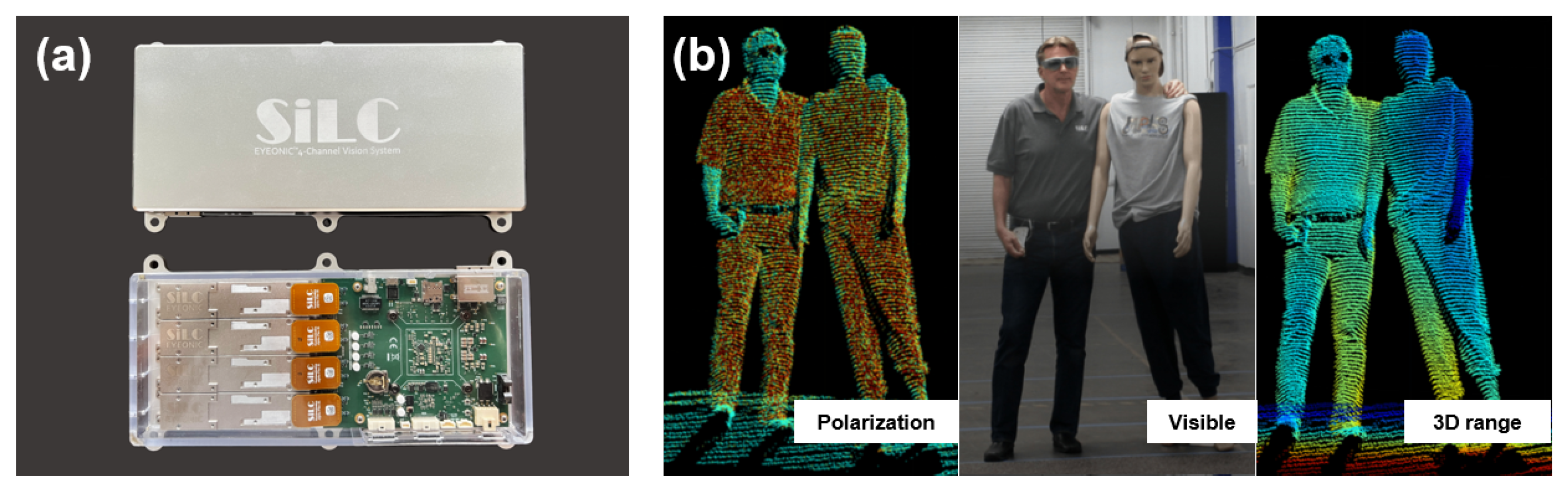
- Eyeonic Vision System The Industry’s Most Compact, Powerful Coherent Machine Vision Solution. Available online: https://www.silc.com/product/ (accessed on 3 September 2023).
- Li, X.; Hu, H.; Zhao, L.; Wang, H.; Han, Q.; Cheng, Z.; Liu, T. Pseudo-polarimetric method for dense haze removal. IEEE Photonics J. 2019, 11, 1–11. [Google Scholar] [CrossRef]
- Hu, H.; Qi, P.; Li, X.; Cheng, Z.; Liu, T. Underwater imaging enhancement based on a polarization filter and histogram attenuation prior. J. Phys. Appl. Phys. 2021, 54, 175102. [Google Scholar] [CrossRef]
- Hu, H.; Lin, Y.; Li, X.; Qi, P.; Liu, T. IPLNet: A neural network for intensity-polarization imaging in low light. Opt. Lett. 2020, 45, 6162–6165. [Google Scholar] [CrossRef] [PubMed]
- Li, X.; Xu, J.; Zhang, L.; Hu, H.; Chen, S.C. Underwater image restoration via Stokes decomposition. Opt. Lett. 2022, 47, 2854–2857. [Google Scholar] [CrossRef]
- Xin, Z.; Changrui, Q.; Jianfeng, S.; Jiang, P.; Qi, W. Research on triggering properties enhancement of polarization detection geiger-mode APD LIDAR. J. Quant. Spectrosc. Radiat. Transf. 2020, 254, 107182. [Google Scholar]
- Lio, G.E.; Ferraro, A. LIDAR and beam steering tailored by neuromorphic metasurfaces dipped in a tunable surrounding medium. Photonics 2021, 8, 65. [Google Scholar] [CrossRef]
- Kim, I.; Martins, R.J.; Jang, J.; Badloe, T.; Khadir, S.; Jung, H.Y.; Kim, H.; Kim, J.; Genevet, P.; Rho, J. Nanophotonics for light detection and ranging technology. Nat. Nanotechnol. 2021, 16, 508–524. [Google Scholar] [CrossRef]
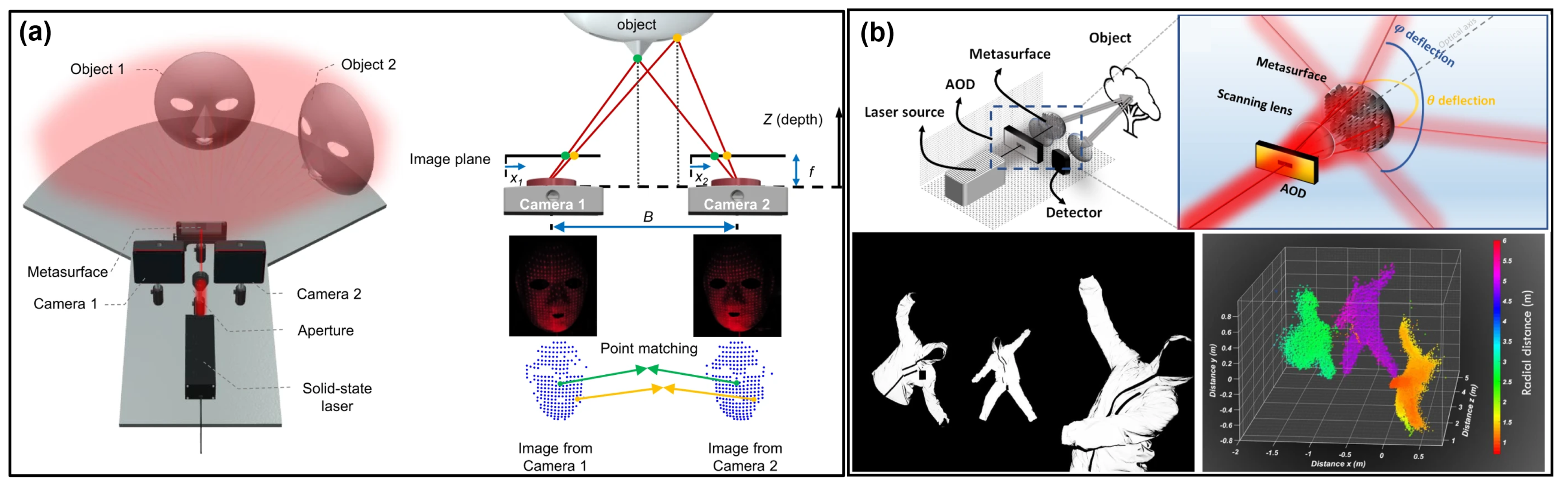
- Kim, G.; Kim, Y.; Yun, J.; Moon, S.W.; Kim, S.; Kim, J.; Park, J.; Badloe, T.; Kim, I.; Rho, J. Metasurface-driven full-space structured light for three-dimensional imaging. Nat. Commun. 2022, 13, 5920. [Google Scholar] [CrossRef]
- Juliano Martins, R.; Marinov, E.; Youssef, M.A.B.; Kyrou, C.; Joubert, M.; Colmagro, C.; Gâté, V.; Turbil, C.; Coulon, P.M.; Turover, D.; et al. Metasurface-enhanced light detection and ranging technology. Nat. Commun. 2022, 13, 5724. [Google Scholar] [CrossRef]
- Liang, Y.; Lin, H.; Koshelev, K.; Zhang, F.; Yang, Y.; Wu, J.; Kivshar, Y.; Jia, B. Full-stokes polarization perfect absorption with diatomic metasurfaces. Nano Lett. 2021, 21, 1090–1095. [Google Scholar] [CrossRef]
- Rubin, N.A.; D’Aversa, G.; Chevalier, P.; Shi, Z.; Chen, W.T.; Capasso, F. Matrix Fourier optics enables a compact full-Stokes polarization camera. Science 2019, 365, eaax1839. [Google Scholar] [CrossRef]


| Scene | Application | Reference |
|---|---|---|
| Precise all-weather retrieval of atmospheric depolarization ratios | [13] | |
| Research on the polarization characteristics of various cloud types | [15,132] | |
| Observe atmospheric ice crystals and water droplets | [39] | |
| Detect the vertical distribution of aerosols and clouds, ascertain cloud particle phase | [45,143] | |
| Identify aerosol and cloud types | [53] | |
| Classification of various aerosol types | [55] | |
| Measure the depolarization ratio of falling snow | [61,131] | |
| Detect high-altitude aerosols | [123] | |
| Atmospheric | Retrieve the nonsphericity of ice particles | [125] |
| Comprehensive atmospheric measurements | [126] | |
| Infer the phase state of submicron particles | [127] | |
| Retrieve micro-physical properties of liquid cloud layers | [128,129] | |
| Analysis of aerosol and water cloud properties | [130] | |
| Detect dust orientation | [142] | |
| Study multi-layer aerosol structures | [146] | |
| Distinguish unique cross-polarization signatures for different tree species | [41] | |
| Detect smoke from forest fires | [108] | |
| Infer three-dimensional surface structure of vegetation | [161] | |
| Earth surface | Characterize the three-dimensional structure of the Earth’s canopy height detection | [162] |
| Study vegetation canopy structure and vegetation cross polarization characterization | [165] | |
| 3D imaging in Urban remote sensing | [170] | |
| Autonomous driving | [176] | |
| Obtain optical properties of seawater at certain depths | [63] | |
| Detection of scattering layers, fish schools, seawater properties, and internal waves | [67] | |
| Oceanographic research | [75] | |
| Observations of aerosols above the ocean | [180] | |
| Understand the optical and microphysical properties of suspended oceanic particles | [181] | |
| Oceanic | Measure the polarized light field in the ocean | [182] |
| Detection of phytoplankton layers | [184,185] | |
| Turbulence measurement | [186,187] | |
| Jellyfish detection | [189,194] | |
| Retrieval of depolarization optical products in the upper ocean | [190] | |
| Marine biological population detection | [191] | |
| Sea surface oil spill detection | [196,197] |
Disclaimer/Publisher’s Note: The statements, opinions and data contained in all publications are solely those of the individual author(s) and contributor(s) and not of MDPI and/or the editor(s). MDPI and/or the editor(s) disclaim responsibility for any injury to people or property resulting from any ideas, methods, instructions or products referred to in the content. |
© 2023 by the authors. Licensee MDPI, Basel, Switzerland. This article is an open access article distributed under the terms and conditions of the Creative Commons Attribution (CC BY) license (https://creativecommons.org/licenses/by/4.0/).
Share and Cite
Liu, X.; Zhang, L.; Zhai, X.; Li, L.; Zhou, Q.; Chen, X.; Li, X. Polarization Lidar: Principles and Applications. Photonics 2023, 10, 1118. https://doi.org/10.3390/photonics10101118
Liu X, Zhang L, Zhai X, Li L, Zhou Q, Chen X, Li X. Polarization Lidar: Principles and Applications. Photonics. 2023; 10(10):1118. https://doi.org/10.3390/photonics10101118
Chicago/Turabian StyleLiu, Xudong, Liping Zhang, Xiaoyu Zhai, Liye Li, Qingji Zhou, Xue Chen, and Xiaobo Li. 2023. "Polarization Lidar: Principles and Applications" Photonics 10, no. 10: 1118. https://doi.org/10.3390/photonics10101118