Optimal Measurement of Telecom Wavelength Single Photon Polarisation via Hong-Ou-Mandel Interferometry

Abstract

The use of statistical estimation theory to boost the metrological performance of the measurement apparatus is becoming increasingly popular in a wide range of applications. Recently, such an approach has been adopted in Hong Ou Mandel interferometry, setting a new record in time delay and polarization measurement. Here, we extend these pioneering experiments in the telecom range to unlock the full potential of the information-based approach combined with a versatile spectral range, aiming for its adoption in fiber-coupled devices of up to hundreds of kilometers long as bobines or optical networks. Our measurement saturates the Cramér-Rao bound and in a long lasting experiment returns an Allan deviation of the polarization angle of 0.002 degs in 1 h of integration time.

1. Introduction

The Hong Ou Mandel (HOM) effect was observed more than 30 years ago, pioneering the quantum technology era.

Namely, when two indistinguishable photons impinge on two ports of a beam splitter (BS), they come out of the same port as a consequence of their bosonic character.

In 1987, Prasad, Scully, and Martienssen published a theoretical paper [1] describing the unitary transformation relating input and output modes of a beam splitter. In the same year [2], Ou, Hong and Mandel deduced the expression of the field at BS output in terms of the input state through diagonal coherent state representation, noting that “with respect to any measurements involving simultaneous photon detections at output ports, the state behaves in the same way as the well-known singlet state for two orthogonally polarized photons”. A few months later [3], the same authors experimentally demonstrated the interference of two identical photons on a BS obtaining the characteristic ’dip’ in coincidence detection at the BS output. The authors presented this result in the context of a precise timing measurement as an extension of classical techniques to measure short pulses using auto-correlation and nonlinear generation.

Lately, increasingly better performances have been achieved thanks to technological advancement [4,5], innovative schemes [6,7,8,9] and light engineering [10,11,12]. The HOM effect is at the heart of many novel applications for quantum light generation [13,14], sensing [15] or fundamental physics tests [16] (see [17] for a comprehensive review).

Advances in quantum estimation theory (QET) led to the introduction of the Fisher Information analysis as a valuable tool in the field of parameter estimation to infer the value of a quantity of interest by inspecting a set of data from the measurement of a different observable, or set of observables [18]. This analysis was first applied to HOM interferometry by Lyons et al. [19]. This innovative approach assisted in reaching a photon time delay resolution of as low as a few attoseconds for a dual arm configuration interferometer, overcoming the previous best resolution obtained in common path configuration [20].

This information-based approach to HOM interferometry for delay measurement has been recently extended to polarization state metrology in the visible wavelength range [21].

In this paper, we extend the results of Harnchaiwat et al. to a telecom range [21] with a fiber-coupled setup, paving the way to future compact and full fiber-coupled applications.

2. Materials and Methods

2.1. Experimental Setup

A twin photon source (TPS, 1. with respect to Figure 1) has been employed to perform polarization-based HOM interferometry. This source is provided with an internal continuous wave (CW) laser pump with a center emission wavelength at 775 nm, illuminating a periodically-poled litium-niobate (PPLN) crystal optimized to achieve the best performances for type-II spontaneous parametric down conversion (SPDC) at 1550 nm when stabilized at a temperature of 33.9 °C.

The twin photon pairs (emmitted from (TPS 1. in Figure 1)) are separated in two parallel paths employing a near-infrared polarizing beam splitter (PBS, 2. in Figure 1) and then coupled in fiber by means of collimating fiber coupler ports.

On one of the two paths, we places a half-wave plate (HWP, 7., as shown in Figure 1) mounted on a rotational stage to align the two polarizations and restore the indistinguishability of the pair. One of the two fiber ports is mounted on a linear translation stage (3. in Figure 1) to compensate for an arms length mismatch. The interference is obtained by coupling each path into a fiber coupled $50/50$ beam splitter input (6. in Figure 1). The BS outputs are coupled to two thermo-electrically cooled single photon avalanche diode (SPAD) detectors (4. in Figure 1) connected to a time-tagging device to record single counts on each detector and coincidence counts between detectors (5. in Figure 1).

Software developed in LabVieW was employed to drive the rotational stage for tuning the polarization mismatch between interfering photons and to collect data from the time tagger.

2.2. Setup Preparation

Before each measurement, the alignment check procedure was carried out to maximize the single counts on either one or the other detector, blinding one fiberport at each time. The second step consists of reaching the center of the HOM dip, characterized by a minimum in the coincidence counts, with all other conditions being equal. This condition is achieved by translating one fiber port with respect to the other until the paths’ length mismatches are compensated for. Misalignments and temperature-induced or mechanical fiber stretch may change the HOM dip center position over time, worsening the degree of distingushability $\alpha$. The measurement routine consists of a LabVieW “while loop”, assigning a value of ${\theta }_i/2$ to the HWP, corresponding to a mismatch angle between interfering photons of ${\theta }_i\in [0^{\circ },{180}^{\circ }]$ then acquires and exports both the single counts of each detector and the coincidence counts to a log file. A single loop consists of $N_s=91$ acquisitions, each one corresponding to an angle ${\theta }_i={\theta }_{i-1}+\mathsf{\Delta }\theta$, where $\mathsf{\Delta }\theta =2^{\circ }$. Each acquisition lasts for $2.1$ s, bringing the whole loop to an overall acquisition time of $191.1$ s. A $5h$-long measurement was performed, corresponding to a log file containing $N_r=100$ loops. A Python script was employed for all subsequent data analyses.

3. Result and Discussion

3.1. Reconstruction of Hong-Ou-Mandel Interference Pattern

Harnchaiwat et al. presented and discussed a theoretical model for Hong–Ou–Mandel interference in polarization-dependent two-photons interferometry in [21]. According to this model, adjusted for linearly polarized photons, the interference function describing the experimental results in the j-th loop (for $j=0,\dots ,N_r-1$) can be written as follows:

$$\frac{N_2\left({\theta }_{ij}\right)}{N_{1ij}}=\frac{1-{\gamma }_j}{3{\gamma }_j+1}·\left(1-{\alpha }_j·(1-{cos}^2({\theta }_{ij}-{\Theta }_j)\right)\forall i=0,\dots ,N_s-1$$

(1)

where $N_2\left({\theta }_{ij}\right)$ represents the number of coincidence counts that occurred during the j-th loop when the HWP was rotated at an angle ${\theta }_i/2$. $N_{1ij}$ represents the number of single count events in the same step (estimated as the sum of the total counts in each detector during the step, once the number of coincidence events and the average dark counts are removed).

Equation (1) therefore helps to obtain the degree of distinguishability ${\alpha }_j$ ($0\le \alpha \le 1$, where $\alpha =1$ represents two identical photons), the optical losses ratio ${\gamma }_j$ (in theory $0\le \gamma \le 1$, but with a detection efficiency of $\eta =20\%$ on each detector the lower bound rises to $\gamma \ge (1-{\eta }^2)=0.96$) and the HOM minimum ${\Theta }_j$ (representing the angle at which the two photons display the lowest residual distinguisability). These parameters are then collected and stored in $N_r$-long vectors (namely $\left\{{\alpha }_j\right\}$, $\left\{{\gamma }_j\right\}$ and $\left\{{\Theta }_j\right\}$).

The overall HOM dip $N_2\left({\theta }_i\right)/N_{1i}$ is plotted in Figure 2, defined as:

$$\frac{N_2\left({\theta }_i\right)}{N_{1i}}=\frac{1}{N_r}\sum _{j=0}^{N_r-1}\frac{N_2\left({\theta }_{ij}\right)}{N_{1ij}}$$

and it is fit with Equation (1). From the $N_r$-fits procedure, the following mean values are retrieved:

$${\gamma }_m=\frac{1}{N_r}\sum _j{\gamma }_j=0.9981,{\alpha }_m=\frac{1}{N_r}\sum _j{\alpha }_j=0.5945,{\Theta }_m=\frac{1}{N_r}\sum _j{\Theta }_j={84.45}^{\circ }$$

3.2. Calibration of the Interferometer

As proven in the previous subsection, the fine tuning of the mismatch angle ${\theta }_i$ affects the coincidence events measured $N_{2i}$ according to Equation (1). The coincidence events can be used to retrieve the mismatch angle between the interfering photons experimentally, which is considered as a parameter (whereas a mismatch angle with an unknown parameter is written as $\tilde{\theta }$).

The standard approach to perform this task [19,21] involves the maximum likelihood estimation (MLE). The conditional probability to observe a certain outcome can be described as $\mathcal{P}(N_0,N_1,N_2|\theta ,\alpha ,\gamma )=P_0^{N_0}{P}_1^{N_1}{P}_2^{N_2}$, where $N_k$ represents the number of times the $k=0,1,2$ detectors click.

The likelihood function, by definition, is $\mathcal{L}(\tilde{\theta },\alpha ,\gamma ,\Theta |N_0,N_1,N_2)=$$\mathcal{P}(N_0,N_1,N_2|\theta ,\alpha ,\gamma ,\Theta )$.

The most likely value of $\tilde{\theta }$ when the outcome $(N_0,N_1,N_2)$ is measured is therefore the one maximizing $\mathcal{L}$, or equivalently $log\mathcal{L}$. Hence:

$${\partial }_{\tilde{\theta }}log\mathcal{L}({\tilde{\theta }}_{MLE},\alpha ,\gamma ,\Theta |N_0,N_1,N_2)=0\Rightarrow N_1{P}_2=P_1{N}_2$$

This leads to ${\tilde{\theta }}_{MLE}$ as:

$${\tilde{\theta }}_{MLE}=\Theta +arccos\left(\sqrt{\frac{N_1-N_2\frac{1+3\gamma }{1-\gamma }}{\alpha (N_1+N_2)}}\right)$$

The vectors $\left\{{\gamma }_j\right\}$, $\left\{{\alpha }_j\right\}$ and $\left\{{\Theta }_j\right\}$ extracted via fit in the previous subsection can be employed to evaluate ${\tilde{\theta }}_{ij}$ according to the following mapping:

$${\tilde{\theta }}_{ij}=\left\{\begin{array}{cc}{\Theta }_j+{90}^{\circ },\hfill & \mathrm{if}{A}_{ij}\le 0\hfill \\ {\Theta }_j,\hfill & \mathrm{if}{A}_{ij}>0\mathrm{and}\sqrt{\frac{A_{ij}}{{\alpha }_j(N_{1ij}+N_{2ij})}}\ge 1\hfill \\ {\Theta }_j+\left(\frac{180}{\pi }\right)arccos\left(\sqrt{\frac{A_{ij}}{{\alpha }_j(N_{1ij}+N_{2ij})}}\right)\hfill & \mathrm{otherwise}\hfill \end{array}\right.$$

(2)

where $A_{ij}=N_{1ij}-N_{2ij}\left(\frac{3{\gamma }_j+1}{1-{\gamma }_j}\right)$.

In free space, where only electro-magnetic self-sustained propagation through air is involved and where there is no polarization distortion, $\tilde{\theta }$ obeys:

$$\tilde{\theta }\left(\theta \right)=\Theta +|\theta -\Theta |$$

This is the case, at least, for areas far from the points of discontinuity of the map in Equation (2). In a setup employing a fiber-coupled BS, however, the previous equation does not necessarily hold true and should be replaced. To expand to greater orders, the underlying polynomial function is the most straightforward way to proceed. The calibration function then becomes:

$$\tilde{\theta }\left(\theta \right)=\Theta +\sum _{l=1}^6{k}_l{|\theta -\Theta |}^l$$

(3)

The matrix ${\left\{\tilde{\theta }\right\}}_{ij}$ obtained from Equation (2) has been therefore employed to evaluate the mean values ${\tilde{\theta }}_i=1/N_r{\sum }_j{\tilde{\theta }}_{ij}$ and their deviations ${\sigma }_i$. Both experimental ${\tilde{\theta }}_i\left({\theta }_i\right)$ and its calibration with Equation (3) ($\Theta ={\Theta }_m$) are reported in Figure 3, together with the free space-case for comparison.

Figure 3 shows that the only non-fitting data points are the ones close to the center angular point in Equations (2) and (3) (i.e., $\theta ={\Theta }_m$).

3.3. Fisher Information and Cramér-Rao Bound

If $\left\{x\right\}$ is a set of possible outcomes and $\mathsf{\Lambda }$ is a parameter influencing these outcomes, the Fisher Information associated with the $\tilde{\mathsf{\Lambda }}$ retrievable via MLE is defined as follows:

$$F_{\mathsf{\Lambda }}=\sum _x\frac{{\left({\partial }_{\mathsf{\Lambda }}\mathcal{P}\left(x\right|\mathsf{\Lambda })\right)}^2}{\mathcal{P}\left(x\right|\mathsf{\Lambda })}$$

where $\mathcal{P}\left(x\right|\mathsf{\Lambda })$ represents the conditional probability that the event x occurs, given the parameter $\mathsf{\Lambda }$. The outcome for the lower bound on the possible variance ${\sigma }^2$ for a parameter $\tilde{\mathsf{\Lambda }}$, evaluated experimentally through $N_{tot}$, is given by the saturation of the following inequality:

$${\sigma }^2\left(\tilde{\mathsf{\Lambda }}\right)\ge \frac{1}{N_{tot}{F}_{\mathsf{\Lambda }}}$$

known as “Cramér-Rao bound”.

If x represents the event of a single detector click, (when both photons come out from the same port of the BS and no coincidence is measured, also referred to as photon bounching) and ${\theta }_i$ is the parameter influencing the outcome, the Fisher Information associated with the experimentally retrieved $\widetilde{{\theta }_i}$ can be calculated as follows [21]:

$$F\left({\theta }_i\right)=\frac{{(1-\gamma )}^2(1+\gamma ){\alpha }^2{sin}^{2}2({\theta }_i-\Theta )}{(1-\alpha {cos}^2({\theta }_i-\Theta ))(1+3\gamma +(1-\gamma )\alpha {cos}^2({\theta }_i-\Theta ))}$$

(4)

The comparison between the standard variances ${\sigma }_{{\tilde{\theta }}_i}^2$ (retrieved from the matrix ${\left\{\tilde{\theta }\right\}}_{ij}$) over the $N_r$ measurements and the theoretical Fisher Information $F\left({\theta }_i\right)$ as reported in Equation (4) can help to investigate how close the system is to the saturation of the Cramér-Rao bound.

$N_{tot}$, the number of observations performed, corresponds to the total number of photons (without losses) involved in the HOM interference, and can be estimated as follows:

$$N_{tot}=\frac{1}{N_r}\sum _j\frac{N_{1ij}+N_{2ij}}{1-{\gamma }_j^2}\approx \frac{1}{N_r}\sum _j\frac{N_{1j}}{1-{\gamma }_j^2}$$

The quantities $1/\left(N_{tot}{\sigma }^2\left({\tilde{\theta }}_i\right)\right)$ have been calculated for each $i=0,\dots ,N_s$ and compared with the Fisher Information function $F({\theta }_i,{\alpha }_m,{\gamma }_m,{\Theta }_m)$. The result is shown in Figure 4.

The comparison shown in Figure 4 proves that the system employing fiber-coupled components is capable of saturating the Cramér-Rao bound for mismatch angles ${\theta }_i$ far from the points of non-derivability in Equation (2). Due to both the piecewise definition of the function ${\tilde{\theta }}_i$, and the intrinsically Poissionan nature of photons generation and detection (where coherent sources are employed), the number of experimental angles ${\theta }_i$ misclassified as either $\Theta$ or $\Theta +{90}^{\circ }$ increases the closer ${\theta }_i$ is to $\Theta$ or to $\Theta \pm {90}^{\circ }$, respectively. At fixed ${\theta }_i$, the more points that are misclassified as, for example, $\Theta +{90}^{\circ }$, the lower the variance $\sigma \left({\theta }_i\right)$. The result is a variance lower than the theoretical limit, but reflecting no underlying physical meaning. Such a feature does not affect the maxima of the Fisher Information function, representing the positions where the measurement should be performed in order to minimize the variance in the outcome.

Note that the red curve in Figure 4 does not represent a fitting function but it is the theoretical model without free parameters.

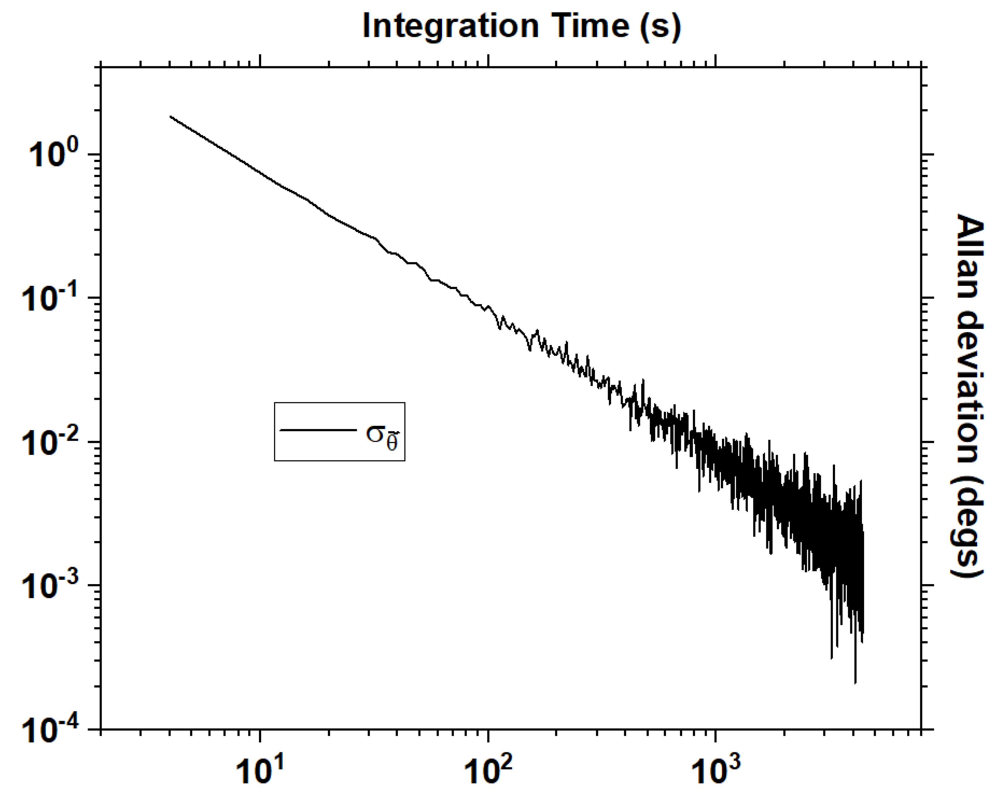
3.4. Allan Deviation Analysis

The measurements presented have been performed at a constant acquisition time-per-point of $\tau =2.1$ s, chosen as a trade-off between an acceptable signal to noise ratio on the photon detection ($\propto \eta \sqrt{N_{1ij}},{\eta }^2\sqrt{N_{2ij}}\propto \tau$) and an acquisition time per ramp $N_s\tau$ that is short enough to consider negligible any fluctuation on $\alpha$, $\gamma$ and $\Theta$ during the single ramp.

A statistical analysis is mandatory for identifying the different noise contributions and for determining signal stability over time. The most widely employed statistical tool to perform this study is the Allan–Werle analysis [22], originally devised for the study of frequency stability of precision oscillators.

With ${\left\{y\right\}}_s$, $s=1\dots M$ as an M-long ensemble of subsequent measurements acquired with an acquisition time ${\tau }_0$, displaying a standard deviation $\sigma \left({\tau }_0\right)={\sigma }_0$, the Allan deviation at acquisition time $\tau =m{\tau }_0$ is calculated as ($K=M/m$):

$$\sigma \left(\tau \right)=\sqrt{\frac{1}{2(K-1)}\sum _{k=1}^{K-1}{\left({\overline{Y}}_{k+1}\left(\tau \right)-{\overline{Y}}_k\left(\tau \right)\right)}^2}$$

where ${\overline{Y}}_k$ is the mean value of the k-th cluster of m values $\{y_{m(k-1)},\dots ,y_{mk}\}$. It is therefore possible to plot $\sigma \left(\tau \right)$ as a function of $\tau =\{{\tau }_0,\dots ,(M/2){\tau }_0\}$, namely the “Allan plot”.

The maximum of the Fisher Information occurs (as can be seen in Figure 4) at ${\theta }_F={123.42}^{\circ }$, and in turn corresponds to a minimum in ${\sigma }_{{\tilde{\theta }}_F}$. ${\theta }_F$ represents the natural candidate to perform a long term stability measurement, starting at ${\tau }_0=2$ s. The Allan deviation plot of ${\sigma }_{{\tilde{\theta }}_F}$ is reported in Figure 5.

The Allan deviation analysis reported in Figure 5 suggests that the system is capable of evaluating ${\tilde{\theta }}_F$ with a deviation ${\sigma }_{{\tilde{\theta }}_F}\left(\tau \right)={0.002}^{\circ }$ after the integration time $\tau =1$ h.

4. Conclusions

In this paper, the study on Hong–Ou–Mandel interference and Fisher Information as a tool for single photon metrology, pioneered by Lyons et al. in [19] and addressed in polarization by Harnchaiwat et al. in [21], has been further extended from the visible to near-infrared range, proving the reliability of this experimental method in the telecommunication range and with fiber-coupled devices. This study proved that even a non-polarization-maintaining system operating in the near-infrared range is capable of achieving an Allan deviation of ${\sigma }_{{\tilde{\theta }}_F}\left(\tau \right)={0.002}^{\circ }$ at $\tau =1$ h integration time during the evaluation of polarization mismatch, and to successfully saturate the Cramér-Rao bound.

The work presented will pave the way towards compact, fiber-coupled single photon metrology via Hong–Ou–Mandel interferometry optimized through Fisher Information analysis.

References

1. Prasad, S.; Scully, M.O.; Martienssen, W. A quantum description of the beam splitter. Opt. Commun. 1987, 62, 139–145. [Google Scholar] [CrossRef]
2. Ou, Z.; Hong, C.; Mandel, L. Relation between input and output states for a beam splitter. Opt. Commun. 1987, 63, 118–122. [Google Scholar] [CrossRef]
3. Hong, C.K.; Ou, Z.Y.; Mandel, L. Measurement of subpicosecond time intervals between two photons by interference. Phys. Rev. Lett. 1987, 59, 2044–2046. [Google Scholar] [CrossRef] [PubMed] [Green Version]
4. Xue, Y.; Yoshizawa, A.; Tsuchida, H. Hong-Ou-Mandel dip measurements of polarization-entangled photon pairs at 1550 nm. Opt. Express 2010, 18, 8182. [Google Scholar] [CrossRef] [PubMed]
5. Tsujimoto, Y.; Wakui, K.; Fujiwara, M.; Sasaki, M.; Takeoka, M. Ultra-fast Hong-Ou-Mandel interferometry via temporal filtering. Opt. Express 2021, 29, 37150. [Google Scholar] [CrossRef]
6. Yepiz-Graciano, P.; Martínez, A.M.A.; Lopez-Mago, D.; Cruz-Ramirez, H.; U’Ren, A.B. Spectrally resolved Hong–Ou–Mandel interferometry for quantum-optical coherence tomography. Photonics Res. 2020, 8, 1023–1034. [Google Scholar] [CrossRef]
7. Jin, R.B.; Gerrits, T.; Fujiwara, M.; Wakabayashi, R.; Yamashita, T.; Miki, S.; Terai, H.; Shimizu, R.; Takeoka, M.; Sasaki, M. Spectrally resolved Hong-Ou-Mandel interference between independent photon sources. Opt. Express 2015, 23, 28836. [Google Scholar] [CrossRef] [Green Version]
8. Kobayashi, T.; Ikuta, R.; Yasui, S.; Miki, S.; Yamashita, T.; Terai, H.; Yamamoto, T.; Koashi, M.; Imoto, N. Frequency-domain Hong–Ou–Mandel interference. Nat. Photonics 2016, 10, 441–444. [Google Scholar] [CrossRef]
9. Orre, V.V.; Goldschmidt, E.A.; Deshpande, A.; Gorshkov, A.V.; Tamma, V.; Hafezi, M.; Mittal, S. Interference of Temporally Distinguishable Photons Using Frequency-Resolved Detection. Phys. Rev. Lett. 2019, 123, 123603. [Google Scholar] [CrossRef] [Green Version]
10. Walborn, S.P.; de Oliveira, A.N.; Pádua, S.; Monken, C.H. Multimode Hong-Ou-Mandel Interference. Phys. Rev. Lett. 2003, 90, 143601. [Google Scholar] [CrossRef]
11. D’Ambrosio, V.; Carvacho, G.; Agresti, I.; Marrucci, L.; Sciarrino, F. Tunable Two-Photon Quantum Interference of Structured Light. Phys. Rev. Lett. 2019, 122, 013601. [Google Scholar] [CrossRef] [PubMed] [Green Version]
12. Kim, H.; Lee, S.M.; Kwon, O.; Moon, H.S. Two-photon interference of polarization-entangled photons in a Franson interferometer. Sci. Rep. 2017, 7, 5772. [Google Scholar] [CrossRef] [PubMed] [Green Version]
13. Chen, Y.; Ecker, S.; Wengerowsky, S.; Bulla, L.; Joshi, S.K.; Steinlechner, F.; Ursin, R. Polarization Entanglement by Time-Reversed Hong-Ou-Mandel Interference. Phys. Rev. Lett. 2018, 121, 200502. [Google Scholar] [CrossRef] [PubMed] [Green Version]
14. Ulanov, A.E.; Fedorov, I.A.; Sychev, D.; Grangier, P.; Lvovsky, A.I. Loss-tolerant state engineering for quantum-enhanced metrology via the reverse Hong–Ou–Mandel effect. Nat. Commun. 2016, 7, 11925. [Google Scholar] [CrossRef] [PubMed] [Green Version]
15. Ndagano, B.; Defienne, H.; Branford, D.; Shah, Y.D.; Lyons, A.; Westerberg, N.; Gauger, E.M.; Faccio, D. Quantum microscopy based on Hong–Ou–Mandel interference. Nat. Photonics 2022, 16, 384–389. [Google Scholar] [CrossRef]
16. Restuccia, S.; Toroš, M.; Gibson, G.M.; Ulbricht, H.; Faccio, D.; Padgett, M.J. Photon Bunching in a Rotating Reference Frame. Phys. Rev. Lett. 2019, 123, 110401. [Google Scholar] [CrossRef] [Green Version]
17. Bouchard, F.; Sit, A.; Zhang, Y.; Fickler, R.; Miatto, F.M.; Yao, Y.; Sciarrino, F.; Karimi, E. Two-photon interference: The Hong–Ou–Mandel effect. Rep. Prog. Phys. 2020, 84, 012402. [Google Scholar] [CrossRef]
18. Paris, M.G.A. Quantum Estimation for Quantum Technology. Int. J. Quantum Inf. 2009, 7, 125–137. [Google Scholar] [CrossRef]
19. Lyons, A.; Knee, G.C.; Bolduc, E.; Roger, T.; Leach, J.; Gauger, E.M.; Faccio, D. Attosecond-resolution Hong-Ou-Mandel interferometry. Sci. Adv. 2018, 4, eaap9416. [Google Scholar] [CrossRef] [Green Version]
20. Branning, D.; Migdall, A.L.; Sergienko, A.V. Simultaneous measurement of group and phase delay between two photons. Phys. Rev. A 2000, 62, 063808. [Google Scholar] [CrossRef]
21. Harnchaiwat, N.; Zhu, F.; Westerberg, N.; Gauger, E.; Leach, J. Tracking the polarisation state of light via Hong-Ou-Mandel interferometry. Opt. Express 2020, 28, 2210. [Google Scholar] [CrossRef] [PubMed]
22. Allan, D. Statistics of atomic frequency standards. Proc. IEEE 1966, 54, 221–230. [Google Scholar] [CrossRef]
Figure 1. Scheme of the experimental setup employed to perform HoM interferometry in polarization. (1.) Twin photon source, (2.) polarizing beam splitter, (3.) linear translation stage, (4.) single photon avalanche diodes detectors (SPADs), (5.) time tagger, (6.) fiber coupled beam splitter and (7.) half-wave plate (HWP) mounted on motorized rotational stage. This figure is obtained via Fusion 360.
Photonics 10 00072 g001
Figure 2. Experimental values for N 2 ( θ i ) / N 1 i (black dots) fitted with Equation (1), shown as red straight curve. On the horizontal axis are reported the mismatch angles θ i = 0 , , 180 .
Photonics 10 00072 g002
Figure 3. θ ˜ ( θ ) (black dots), its best fit with calibration curve from Equation (3) (blue straight curve), and the free space limit (dotted magenta curve).
Photonics 10 00072 g003
Figure 4. Experimentally retrieved 1 / ( N t o t σ 2 ( θ ˜ i ) ) as a function of θ i , black dots. Theoretical model without free parameters F ( θ i , α m , γ m , Θ m ) (straight red curve).
Photonics 10 00072 g004
Figure 5. Allan deviation of θ ˜ F , evaluated from long-term measurement.
Photonics 10 00072 g005
Disclaimer/Publisher’s Note: The statements, opinions and data contained in all publications are solely those of the individual author(s) and contributor(s) and not of MDPI and/or the editor(s). MDPI and/or the editor(s) disclaim responsibility for any injury to people or property resulting from any ideas, methods, instructions or products referred to in the content.