Recognizable Languages of k-Forcing Automata

Abstract

In this study, we show that automata theory is also a suitable tool for analyzing a more complex type of the k-forcing process. First, the definition of k-forcing automata is presented according to the definition of k-forcing for graphs. Moreover, we study and discuss the language of k-forcing automata for particular graphs. Also, for some graphs with different k-forcing sets, we study the languages of their k-forcing automata. In addition, for some given recognizable languages, we study the structure of graphs. After that, we show that k-forcing automata arising from isomorph graphs are also isomorph. Also, we present the style of words that can be recognized with k-forcing automata. Moreover, we introduce the structure of graphs the k-forcing automata arising from which recognize some particular languages. To clarify the notions and the results obtained in this study, some examples are submitted as well.

1. Introduction

Graph theory was introduced by Leonhard Euler in 1736 to solve the Königsberg bridge problem. Since then, this theory has been used to describe many fundamental issues or phenomena in operations research, chemistry, computer science, and social science. Numerous groups of authors have introduced and studied various graph generation models from different perspectives [1,2,3,4,5]. Additionally, it has been used in communication roads of cities, city maps, etc. The notion of a zero forcing set of a simple graph was introduced in [6] to bound the minimum rank for numerous families of graphs. Zero forcing parameters were further studied and applied to the minimum rank problem in [7,8].

On the other hand, different types of automata demonstrate rich and exciting properties that could be applied to modeling and simulating different types of epidemics, and we refer to [2,9,10,11,12,13] for details. In addition, there has been limited research on the application of automata theory to analyze disease propagation. So, here, we bring an interdisciplinary approach, including graph theory and automata theory, to analyze a type of the k-forcing process.

Today, studying the behavior of infectious diseases in different societies has the highest research priority to prevent and control them. It seems that some branches of mathematics, including automata theory, can help us to do this research. It has already been shown that the behavior of a kind of zero forcing process can be analyzed by forcing automata. Past research has shown that a simple type of the zero forcing process could be analyzed by deterministic finite-state automata. The k-forcing process is the generalization of the zero forcing process. In this paper, we show that it is also possible to analyze and model the k-forcing process by finite-state automata. First, we define the k-forcing automaton according to the propagation steps and the conditions under which the k-forcing process is transmitted. Then, we demonstrate that the language of k-forcing automaton enables us to compare different k-forcing processes within a given network or across different networks. Recently, Golmohamadian, Zahedi and Soltankhah introduced a model of graph automata [10]. Further, the L-graph notion based on the residuated lattice was introduced, and its applications were presented and discussed [14]. Moreover, the L-fuzzy automaton known as the L-graph automaton [14] was introduced.

The structure of the paper is as follows. In Section 3, we introduce the definitions and some properties of the graph, zero forcing set, and automata. In Section 4, the definition of k-forcing automata is presented according to the definition of k-forcing for graphs. After that, the k-forcing grammar is defined. In Section 5, first, languages of k-forcing automata for some graphs are discussed. Further, for a given graph $G_1$, a new graph is presented, say $G_2$, such that k-forcing automata of $G_1$ and l-forcing automata of $G_2$ have the same language. Also, for some graphs with various k-zero forcing sets, we study the languages of their k-forcing automata. Moreover, we show that if two graphs G and H are isomorphic, then there are two k-forcing sets $Z^k\left(G\right)$ and $Z^k\left(H\right)$ such that their k-forcing automata are isomorphic. In Section 6, the style of words that can be recognized with k-forcing automata is studied. Moreover, we introduce the structure of graphs from which the k-forcing automata arise, producing particular languages.

2. Notation

We need the following items to better understand the next sections [15]:

• $\mathcal{A}=(Q,A,\phi ,I,T)$ is an automata, where Q is a states set, A is an alphabet set, $\phi :Q\times A\to Q$ is a transition function, $I\subseteq Q$ is an initial states set, and $T\subseteq Q$ is a final states set.
• The cardinality of Q is denoted by $\left|Q\right|$.
• Let V be a nonempty set. Then $V^{*}$ is the free monoid over V with the empty word, $\lambda$, as the identity of $V^{*}$. Moreover, let $V^{+}=V^{*}\setminus \left\{\lambda \right\}$.
• $G=(V,E)$ is a graph, where V is the set of vertices and E is the set of edges.
• A simple graph is a graph with no loops or multiple edges.
• A complete graph is a simple graph such that each pair of distinct vertices is adjacent.
• Graph G is connected if every pair of vertices belongs to a path.
• The degree of a vertex is the number of edges with that vertex as an end-point.
• We say that two vertices a and b of a graph G are adjacent if there is an edge $ab$ joining them.
• The initial color of each vertex in graph G is black (colored) or white (non-colored). The union of colored and non-colored vertices is equal to the set of vertices of the graph G.

3. Preliminaries

A zero forcing process is an instance of an irreversible propagation process on graphs or networks. The zero forcing process is defined as follows for simple, finite, and undirected graphs. The initial color of each vertex in graph G is black or white (in this paper, the black vertex is an infected member, and the white vertex is a healthy member). Let $uv$ be an edge in graph G. When we say that u forces v, denoted by $u\to v$, we mean that the edge uv is an enforcing one, that is, if u is a vertex that is black and u has a single white neighbor, like v, then we alter the color of v to black; this law is called the law of color change (or the conditions in which the disease is transmitted).

The initial coloring of G involves a set of vertices being black and all other vertices being white; repeating the color-change rule until no more changes are possible leads to the derived set of all black vertices. If the derived set for a given initial subset of black vertices is the entire vertex set of the graph, a zero forcing set is the name given to the initial black vertices. The zero forcing process is a process that changes the color of all white vertices to black vertices [6,16].

It should be noted that the smallest zero forcing set for the graph is the size of the graph’s zero forcing number. $\left|Z\right(G\left)\right|$ is used to denote the zero forcing number in a graph G.

Definition 1 

([17]). Let $G=(V,E)$ be a graph. A zero forcing finite automata (Z-F-finite automata) is a five-tuple machine denoted by $\mathcal{A}=(Q,A,\phi ,I,T)$, where

1. 

$Q=V$ is the finite set of states,

2. 

$A=\{f,n\}$ is the set of alphabet,

3. 

$\phi :Q\times A\to P\left(Q\right)$ is the transition function, where if vertex u forces vertex v in G, then we define $\phi (u,f)=v$ in $\mathcal{A}$ and, if $uv\in E$ and u and v do not force each other, then $\phi (u,n)=v$ and $\phi (v,n)=u$,

4. 

$I=Z\left(G\right)$ is the set of initial states,

5. 

T is the set of final states, which $u\in T$ if and only if u does not force any vertex.

Naturally, φ can be extended to ${\phi }^{*}:Q\times A^{*}\to P\left(Q\right)$.

Definition 2. 

([18]). Let $k\ge 1$ be an integer and let G be a graph containing either colored or non-colored vertices, and let $S\subseteq V$ be the set of all initially colored vertices. The k-coloring rule is defined by the following: if v is a colored vertex with k or fewer uncolored neighbors, then we change the color of the non-colored neighbors of v. If all vertices are colored by repeatedly applying the k-coloring rule, then it is said that S is a k-forcing set. The k-forcing number, $|Z^k\left(G\right)|$, is the cardinality of a minimum k-forcing set of G.

A k-forcing process is a generalization of the zero forcing process and is an example of an irreversible propagation process on graphs or networks. The following example helps us to better understand why the k-forcing process is an epidemic.

Example 1. 

Let G be the graph in Figure 1 and $Z=\{v_1,v_7\}$ and $k=2$. The shapes in Figure 1 show that how the 2-forcing process happens in the graph G and how the color of all white vertices change to black. Figure 1 also shows that Z is a 2-forcing set.

Definition 3 

([15]). A graph G is a bipartite graph if its vertex set can be divided into two disjoint sets A and B, where each edge of G joins the vertices a and b.

Definition 4 

([15]). Let G and H be two simple graphs. A homomorphism from G to H is a surjection $f:V_G\to V_H$ where $ab\in E_G$ if and only if $f\left(a\right)f\left(b\right)\in E_H$. f is called an isomorphism if and only if f is a homomorphism that is one–one.

Definition 5 

([17]). Let ${\mathcal{A}}_1=(Q_1,A,\phi ,I_1,T_1)$ and ${\mathcal{A}}_2=(Q_2,A,\phi ,I_2,T_2)$ be two automata. A homomorphism from ${\mathcal{A}}_1$ onto ${\mathcal{A}}_2$ is a surjection $g:Q_1\to Q_2$, where, for every $p,p^{\prime }\in Q_1$, and $a\in A$, the following conditions hold:

• $p\in I_1$ if and only if $g\left(p\right)\in I_2$,
• $\phi (p,a)=p^{\prime }$ if $\phi (g\left(p\right),a)=g\left(p^{\prime }\right)$,
• $p\in T_1$ implies that $g\left(p\right)\in T_2$.

g is called an isomorphism if and only if g is a homomorphism that is one–one and $p\in T_1$ if and only if $g\left(p\right)\in T_2$.

Definition 6 

([19]). A formal grammar is a quadruple $\mathrm{\Gamma }=(S,A,\pi ,\sigma )$, where S is a finite symbols set called the vocabulary of Γ, A is a nonempty subset of S called the terminal alphabet of Γ, π is a finite subset of ${(S-A)}^{+}\times S^{*}$, and $\sigma \in S-A$. The elements $(\alpha ,\beta )$ of π are called the productions of Γ and we write $\alpha \to \beta$ whenever $(\alpha ,\beta )\in \pi$.

4. k-Forcing Automata

In this section, first, we define k-forcing automata by using Definition 2. In the following, we present a k-forcing grammar as well.

Definition 7. 

Let $G=(V,E)$ be a graph and $Z^k\left(G\right)$ be a k-forcing set of it. A k-forcing automata (k-F-Automata) is a five-tuple machine $\mathit{A}\left(Z^k\left(G\right)\right)=(Q,A,\phi ,I,T)$, where

1. 

$Q=V$ is the set of states of $\mathit{A}\left(Z^k\left(G\right)\right)$,

2. 

$A=\{f,n\}$ is the alphabet set,

3. 

$\phi :Q\times A\to P\left(Q\right)$ is a transition function, where, if vertex q forces vertex $q^{\prime }$ in graph G, then we define $q^{\prime }\in \phi (q,f)$ in $\mathit{A}\left(Z^k\left(G\right)\right)$ and, if $q{q}^{\prime }\in E$ and q and $q^{\prime }$ do not force each other, then we consider $q^{\prime }\in \phi (q,n)$ and $q\in \phi (q^{\prime },n)$ in $\mathit{A}\left(Z^k\left(G\right)\right)$,

4. 

$I=Z^k\left(G\right)\subseteq V$ is the initial states set,

5. 

T is the final states set, in which $q\in T$ if and only if q does not force each vertex.

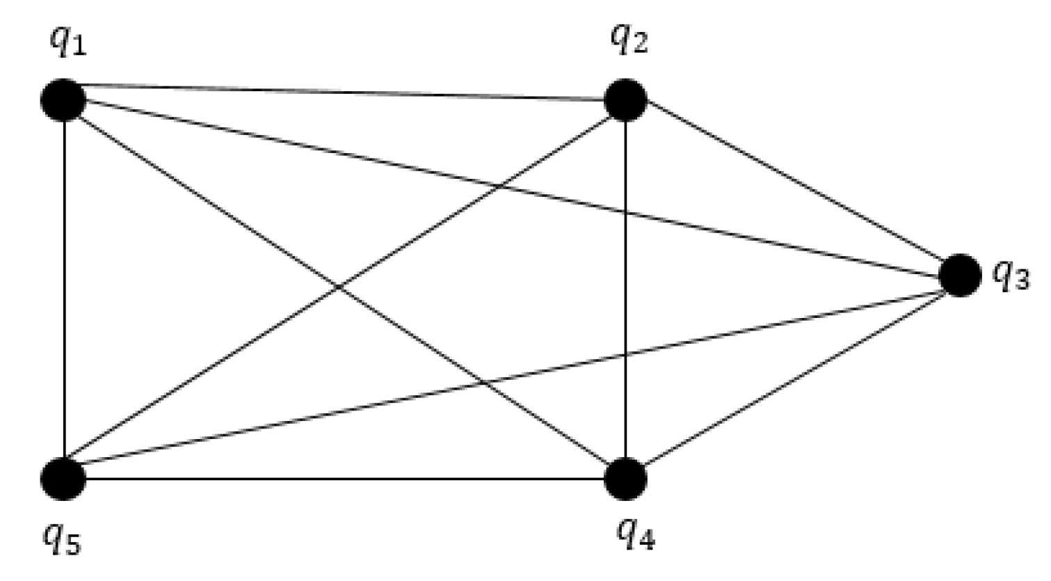
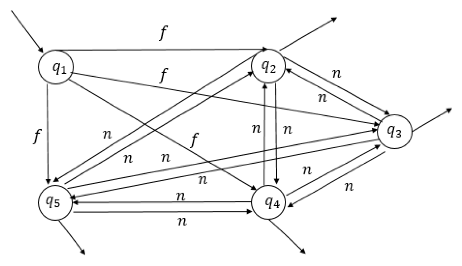
Example 2. 

Consider graph G as in Figure 2. Let $k=2$ and $Z_1^2\left(G\right)=\left\{q_1\right\}$. Clearly, $q_1$ forces $q_2$ and $q_5$, after that $q_2$ forces $q_3$ and $q_4,$ and, at the same time, $q_5$ forces $q_4$. Now, all vertices are colored. Then $q_3$ and $q_4$ do not force each other. Therefore, we have $\mathit{A}\left(Z_1^2\left(G\right)\right)$, as in Figure 3. Now, we consider $Z_2^2\left(G\right)=\left\{q_3\right\}$. We have $\mathit{A}\left(Z_2^2\left(G\right)\right)$, as in Figure 4. We notice that $\left\{q_2\right\}$ and $\left\{q_4\right\}$ are not 2-forcing sets, also $\left\{q_3\right\}$ is not a zero forcing set for graph G.

It should be noted that k-forcing automata is a generalization of Z-F-automata, see [17].

Definition 8. 

Let $\mathit{A}\left(Z^k\left(G\right)\right)=(Q,A,\phi ,I,T)$ be a k-forcing automata. The language of $\mathit{A}\left(Z^k\left(G\right)\right)$ is defined to be the set $L\left(\mathit{A}\left(Z^k\left(G\right)\right)\right)=\{w\in A^{*}|\phi (i,w)\in T,\exists i\in I\}$, where $1\le k\le \left|Q\right|-1$.

Example 3. 

Consider graph G, as in Figure 2. By considering $Z_1^2\left(G\right)=\left\{q_1\right\}$, clearly, $L\left(\mathit{A}\left(Z_1^2\left(G\right)\right)\right)=f^2{n}^{*}$. Now, we consider $Z_2^2\left(G\right)=\left\{q_3\right\}$. Obviously, $L\left(\mathit{A}\left(Z_2^2\left(G\right)\right)\right)=f{n}^{*}f{n}^{*}$.

Example 4. 

Consider graph G, as in Figure 5, and 2-forcing set $Z^2\left(G\right)=\{q_1,q_2,q_3\}$. Then, we have $\mathit{A}\left(Z^2\left(G\right)\right)$, as in Figure 6. Clearly, $L\left(\mathit{A}\left(Z_2^2\left(G\right)\right)\right)=n^{*}f{n}^{*}$. Now, let $Z^3\left(G\right)=\{q_1,q_2\}$ be a 3-forcing set for graph G. Then, we have $\mathit{A}\left(Z^3\left(G\right)\right)$, as in Figure 7, also, the language of this automata is equal $n^{*}f{n}^{*}$. By considering $Z^4\left(G\right)=\left\{q_1\right\}$, we have $\mathit{A}\left(Z^4\left(G\right)\right)$, as in Figure 8. Obviously, $L\left(\mathit{A}\left(Z^4\left(G\right)\right)\right)=f{n}^{*}$. Moreover, in [17], we can see $L\left(\mathit{A}\left(Z^1\left(G\right)\right)\right)=n^{*}f$.

If the forcing set $S\subseteq V$ of black (infected) vertices is fixed, the resulting automata do not need to be unique (as just mentioned): it depends on the order in which vertices from outside the current set S are colored in black. For the same graph $G=(V,E)$ and the same k-forcing set $S\subseteq V$, the k-forcing automata and language are unique. So, the language only depends on the given graph G and the given forcing set S of its vertices.

By utilizing Definition 7, we can present k-forcing grammar for a given graph $G=(V,E)$ and k-forcing set $Z^k\left(G\right)$, $1\le k\le n-1,\left|G\right|=n$. A k-forcing grammar (k-F grammar) is a quadruple ${\mathrm{\Gamma }}_{Z^k\left(G\right)}=(S,A,\pi ,\sigma )$, where

• $S=V\cup \{f,n\}\cup \left\{\sigma \right\}$ is the symbols set.
• $\{f,n\}$ is the alphabet set.
• Every production rule is of the following form:

  (I)

  $q^{\prime }\to f{q}^{″}$, whenever $q^{\prime }$ forces $q^{″}$ in graph G.

  (II)

  $q^{\prime }\to n{q}^{″}$, whenever $q^{\prime }$ does not force $q^{″}$ and $q^{\prime }{q}^{″}\in E$.

  (III)

  $q^{\prime }\to 1$, if $q^{\prime }$ does not force any vertex.

  (IV)

  $\sigma \to q$, whenever $q\in Z^k\left(G\right)$.

Example 5. 

Consider graph G, as in Figure 5. By considering the 2-forcing set $Z^2\left(G\right)=\{q_1,q_2,q_3\}$, we have 2-forcing grammar ${\mathrm{\Gamma }}_{Z^2\left(G\right)}$ as follows:

$$\begin{array}{cc}\hfill & \sigma \to q_1,\sigma \to q_2,\sigma \to q_3,q_1\to n{q}_2,\hfill \\ \hfill & q_2\to n{q}_1,q_2\to n{q}_3,q_3\to n{q}_2,q_1\to f{q}_5\hfill \\ \hfill & q_1\to f{q}_4,q_1\to n{q}_3,q_3\to n{q}_1,q_2\to f{q}_5\hfill \\ \hfill & q_2\to f{q}_4,q_3\to f{q}_4,q_3\to f{q}_5,q_4\to n{q}_5,\hfill \\ \hfill & q_5\to n{q}_4,q_4\to 1,q_5\to 1.\hfill \end{array}$$

It is clear that k-forcing grammar is a regular grammar.

Note 1. 

For every complete graph, it is obvious that every state in its k-forcing automata is neither the initial state nor the final state.

Note 2. 

Let G be a complete graph and $\left|G\right|=n$. Then, for every k-forcing set $Z^k\left(G\right)$, we have $|Z^k\left(G\right)|=n-k$, where $1\le k\le n-1$.

5. Recognizable Languages

In this section, first, we discuss recognizable languages and study the features of some graphs that can be recognized by these languages. For some kinds of recognizable languages, we present some graphs as well. Moreover, we present a general language and show that languages of k-forcing automata follow this pattern. To clarify the concepts some examples are also given.

Definition 9. 

Let $L\subseteq A^{*}$. We say that L is a recognizable language if there exists a graph G, such that $L\left(\mathit{A}\left(Z^k\left(G\right)\right)\right)=L$, for some k-forcing set $Z^k\left(G\right)$.

Theorem 1. 

Let $L=f^m,m\ge 2$. Then there exists a graph G such that $L\left(\mathit{A}\left(Z^2\left(G\right)\right)\right)=f^m$, for every 2-forcing set $Z^2\left(G\right)$. Moreover, G is a 2-regular graph in which $\left|G\right|=2km$ and every component of it is a 2-regular graph, such that $L\left(\mathit{A}\left(Z^2\left(G^{\prime }\right)\right)\right)=f^m$, for every component $G^{\prime }$ of G and $k\in N$.

Proof. 

By using Theorem 12, it is evident that for a 2-regular connected graph G such that $\left|G\right|=2m$, we have $L\left(\mathbf{A}\left(Z^2\left(G\right)\right)\right)=f^m$, for every 2-forcing set $Z^2\left(G\right)$. Let G be a path, so, by considering $Z^2\left(G\right)=\left\{p\right\}$ and $Z^2\left(G\right)=\left\{p^{\prime }\right\}$, such that $d\left(p\right)=2$ and $d\left(p^{\prime }\right)=1$, where $p,p^{\prime }$ belong to the set of vertices of G, we do not have the same language $f^m$. On the other hand, if there exists a vertex in G such that its degree is more than two, by choosing every $Z^2\left(G\right)$, at least one of the edges of that vertex creates $n^{*}$, which is a contradiction. So, G is a 2-regular graph. We suppose graph G has several components. If at least two components of G have different numbers of vertices, then we have $L\left(\mathbf{A}\left(Z^2\left(G\right)\right)\right)=f^m\cup f^{m^{\prime }}$, where $f^m$ and $f^{m^{\prime }}$ are the languages of these components, which is a contradiction too. Hence, the claim holds. □

Theorem 2. 

Let $L=f^m$. Then there is not any graph with less than m vertices in which the language of k-forcing automata of it be L, for every k-forcing set $Z^k\left(G\right)$.

Proof. 

Let G be a graph and $Z^k\left(G\right)$ be a k-forcing set of G. Since $L=f^m$, then there are m forces in graph G. By considering Definition 2, the claim is clear. □

Theorem 3. 

Let $L=f^m{n}^{*},m\ge 2$. Then there is a graph G such that $L\left(\mathit{A}\left(Z^2\left(G\right)\right)\right)=f^m{n}^{*}$, for every 2-forcing $Z^2\left(G\right)$. Also, G is a 2-regular graph such that $\left|G\right|=k(2m+1)$, graph G has k components, and every component $G^{\prime }$ of G is a 2-regular graph in which $L\left(\mathit{A}\left(Z^2\left(G^{\prime }\right)\right)\right)=f^m{n}^{*}$, where $k\ge 1$.

Proof. 

According to Theorem 12, the first part of the claim is clear. Graph G cannot be as a path, since, for every 2-forcing $Z^2\left(G\right)$, k-forcing automata of the graph cannot create $n^{*}$. On the other hand, since $L=f^m{n}^{*}$, we have $\left|Z\right(G\left)\right|=1$, by considering the hypothesis, we have to have m forces at first and these forced vertices must not be adjacent since they create $f^{m^{\prime }}{n}^{*}{f}^{m^{″}}$ and it is a contradiction. After that, for creating $n^{*}$, we have to have at least two final states and these states must be adjacent. So, the graph G is 2-regular. Now, we have two cases: The first one, graph G is connected, so G is a 2-regular connected graph and $\left|G\right|=2m+1$. In the last case, G is not connected. Then G has k components such that $L\left(\mathbf{A}\left(Z^2\left(G^{\prime }\right)\right)\right)=f^m{n}^{*}$, for every component graph $G^{\prime }$ of G and $|G^{\prime }|=2m+1$. Therefore, $\left|G\right|=k(2m+1)=2km+k$. Hence, the claim holds. □

Corollary 1. 

Let $L=f^m{n}^{*}$. Then there is a graph G such that $\left|G\right|=m+2$ and $L\left(\mathit{A}\left(Z^k\left(G\right)\right)\right)=f^m{n}^{*}$, for some k-forcing set $Z^k\left(G\right)$, $k\ge 2$. Also, there does not exist any graph, say H, with fewer vertices in which $L\left(\mathit{A}\left(Z^k\left(H\right)\right)\right)=f^m{n}^{*}$.

Corollary 2. 

Let $L=n^{*}{f}^m{n}^{*}$. Then there does not exist any graph G such that $L\left(\mathit{A}\left(Z^l\left(G\right)\right)\right)=n^{*}{f}^m{n}^{*}$, where $Z^l$ is an l-forcing set of G and $\left|G\right|\le m+1$.

Corollary 3. 

Let $L=n^{*}{f}^m{n}^{*}$. The smallest graph G such that $L\left(\mathit{A}\left(Z^1\left(G\right)\right)\right)=n^{*}{f}^m{n}^{*}$ has $m+2$ vertices, where $Z^1\left(G\right)$ is a zero forcing set for graph G.

Theorem 4. 

Let $L=f^m{n}^{*}{f}^{m^{\prime }}$. Then for every graph G in which $L\left(\mathit{A}\left(Z^k\left(G\right)\right)\right)=L$, graph G has at least two vertices of degree at least two, where $Z^k\left(G\right)$ is a k-forcing set for graph G and $k\ge 2$.

Proof. 

Let G be a graph. For creating $f^m$, we have to have m force; for creating $n^{*}$, we have to have at least two adjacent vertices that do not force each other. Since these vertices are forced by other vertices and also have to force other vertices, the degree of these vertices is at least three. Hence, the claim holds. □

Corollary 4. 

Let $L=f^m{n}^{*}{f}^{m^{\prime }}$. Then the smallest graph G such that $L\left(\mathit{A}\left(Z^k\left(G\right)\right)\right)=L$ has at least $m+m^{\prime }+2$ vertices, where $Z^k\left(G\right)$ is a k-forcing set for the graph and $k\ge 2$.

Theorem 5. 

Let $L_1=n^{*}{f}^l$ and $L_2=f^l{n}^{*}$. There is no graph G such that $L\left(\mathit{A}\left(Z^{m-1}\left(G\right)\right)\right)=L_1$ or $L\left(\mathit{A}\left(Z^1\left(G\right)\right)\right)=L_2$, where $\left|G\right|=m$.

Proof. 

Let $L_1=n^{*}{f}^l$. Clearly, for every graph G, $|Z^{m-1}\left(G\right)|=1$, where $\left|G\right|=m$. Since we have only one member in $Z^{m-1}\left(G\right)$, it is not possible to create $n^{*}$. For the rest of the claim, see [17]. □

Theorem 6. 

For every graph G such that $L\left(\mathit{A}\left(Z^1\left(G\right)\right)\right)=n^{*}{f}^m$, graph G has at least three vertices with at least two degrees.

Proof. 

Let $L=n^{*}{f}^m$. For creating $n^{*}$, we must have $|Z^1\left(G\right)|\ge 2$; it means that at least two initial states of $\mathbf{A}\left(Z^1\left(G\right)\right)$ are adjacent. Then the degree of vertices in $Z^1\left(G\right)$ is at least two. For creating $f^m$, we have to have at least m other vertices. We have two cases:

(a)

The initial vertices have the same adjacent vertices, then the claim holds.

(b)

The initial vertices do not have the same adjacent vertices; to create $f^m$, all vertices in $Z^1\left(G\right)$ have similar paths and, finally, all these paths are common in a vertex; otherwise, the graph is a path and it is a contradiction.

Hence, the claim holds. □

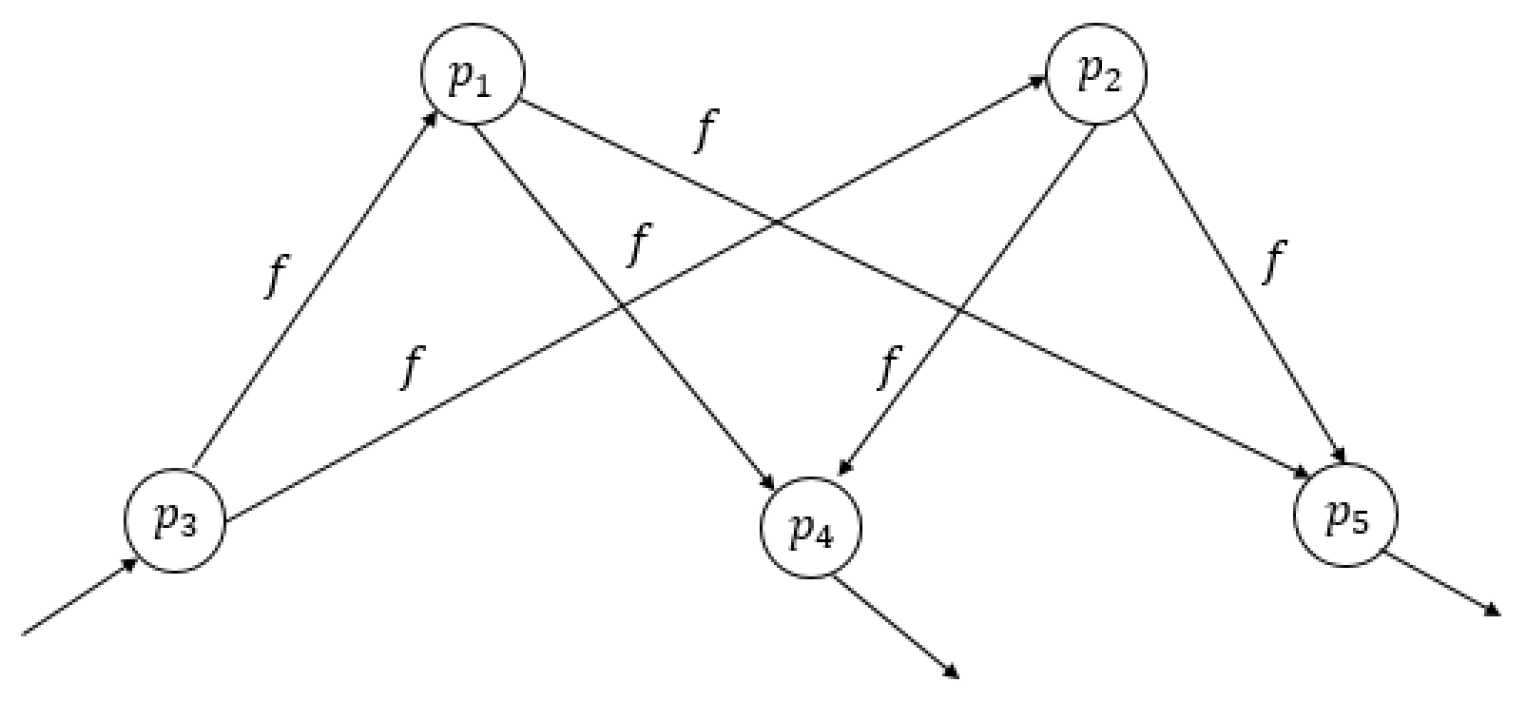
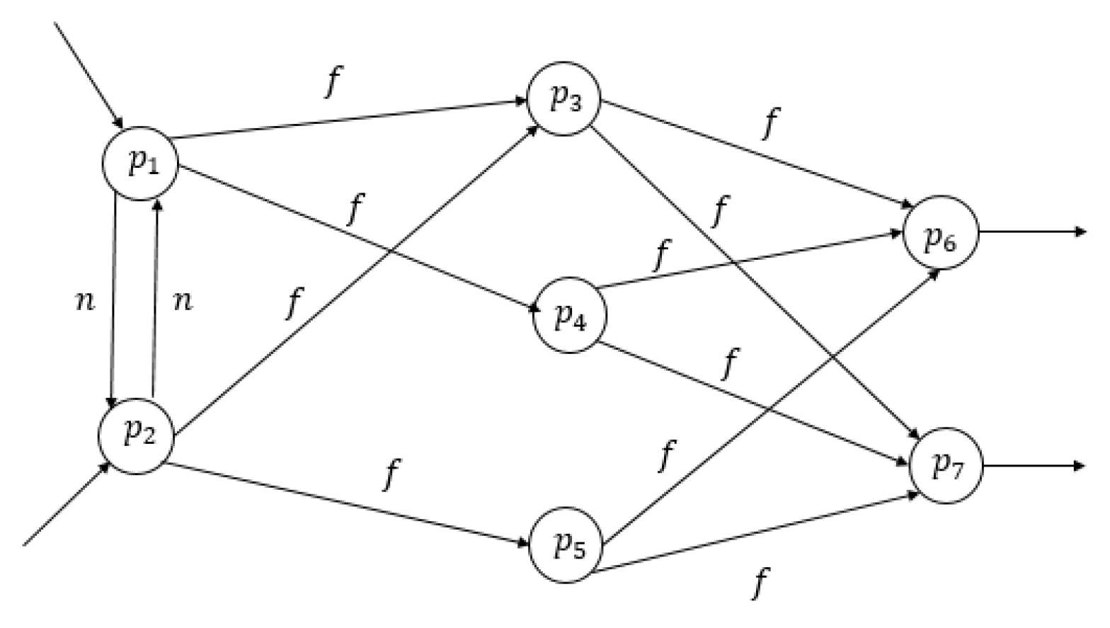
Example 6. 

Let $L=n^{*}{f}^2$. By using the proof of Theorem 6, we have the graph G, as in Figure 9. By considering $Z^1\left(G\right)=\{p_1,p_2\}$, the language of 1-forcing automata of it is $n^{*}{f}^2$. Also, we can consider graph G, as in Figure 10. With regard to choosing $Z^1\left(G\right)=\{p_1,p_2,p_3\}$, the language of 1-forcing automata of it is $n^{*}{f}^2$.

Corollary 5. 

Let $L=n^{*}{f}^m$. Then there exists a graph G such that $\left|G\right|=m+2$ and $L\left(\mathit{A}\left(Z^1\left(G\right)\right)\right)$ = $n^{*}{f}^m$, for the some forcing set $Z^1\left(G\right)$. Also, there is no graph H with fewer states that $L\left(Z^1\left(H\right)\right)=n^{*}{f}^m$.

Theorem 7. 

Let L be a recognizable language and G be the corresponding graph. Then for $k=2,\dots ,\left|G\right|-2$, we have $L=n^{*}{f}^l{n}^{*}{\left(n^{*}{f}^{l^{\prime }}{n}^{*}\right)}^{*}$, for some integers $l,l^{\prime }$.

Proof. 

Let G be a graph such that $L\left(\mathbf{A}\left(Z^k\left(G\right)\right)\right)=L$, for some k-forcing set $Z^k\left(G\right)$. Without loss of generality, let $k=2$ and $w=a_1{a}_2\dots a_n\in L$. Then $\phi (i,w)\in T$, for some $i\in Z^2\left(G\right)$. So, we have a path defined as follows:

$$i\stackrel{a_1}{\to }{q}_1\stackrel{a_2}{\to }{q}_2\to \dots \stackrel{a_n}{\to }{q}_n\in T,$$

There are two cases for two vertices i and $q_1$. In the first case, i forces $q_1$, so we have $\phi (i,f)=q_1$. Therefore, $a_1=f$. In the last case, i does not force $q_1$, then $\phi (i,n)=q_1$ and $\phi (q_1,n)=i$, so it creates $n^{*}$. We proceed in the same way for the rest of the path. Hence, the claim is clear. □

6. Languages of k-Forcing Automata

In the first part of this section, we study the language of k-forcing automata for several graphs such as complete graphs, bipartite graphs, and regular graphs. After that, for a given graph $G_1$, we present a new graph, say $G_2$, such that k-forcing automata of $G_1$ and l-forcing automata of $G_2$ have the same language and k and l are not necessarily the same. Also, we present some examples to clarify these new notions. In [17], Shamsizadeh et al. show that if G is a complete graph where $\left|G\right|\ge 3$, then for every $m-1$-forcing set $Z^{m-1}\left(G\right)$, $L\left(\mathbf{A}\left(Z^{m-1}\right)\right)=n^{*}f$. Now, by considering the k-forcing set $Z^k\left(G\right)$, we can extend the language.

Theorem 8. 

Let G be a complete graph such that $\left|G\right|=m$. Then for each k-forcing set $Z^k\left(G\right)$, where $2\le k\le m-2$, we have $L\left(A\left(Z^k\left(G\right)\right)\right)=n^{*}f{n}^{*}$, and $L\left(\mathit{A}\left(Z^{m-1}\right)\right)=f{n}^{*}$.

Proof. 

The language $L\left(\mathbf{A}\left(Z^k\left(G\right)\right)\right)=n^{*}f{n}^{*}$ consists of three parts, $n^{*},f$, and $n^{*}$. Let G be a complete graph and $Z^k\left(G\right)$, $2\le k\le m-2$ be a k-forcing set of G. Since $|Z^k\left(G\right)|\ge 2$, its k-F-automata has at least two adjacent initial states and they create $n^{*}$ (first part of $n^{*}f{n}^{*}$). On the other hand, every state belonging to $Z^k\left(G\right)$ forces the rest of the states and it creates f (second part of $n^{*}f{n}^{*}$). Also, by utilizing Note 1, at least two states of $\mathbf{A}\left(Z^k\left(G\right)\right)$ are final. Then they create $n^{*}$ because they are adjacent. Therefore, $L\left(\mathbf{A}\left(Z^k\left(G\right)\right)\right)=n^{*}f{n}^{*}$.

Now, let $Z^{m-1}\left(G\right)$ be an $(m-1)$-forcing set for G. Then $|Z^{m-1}\left(G\right)|=1$. So, we have one initial state; it forces the other vertices and it creates f. Since the final states are adjacent, then they create $n^{*}$. Therefore, $L\left(\mathbf{A}\left(Z^{m-1}\left(G\right)\right)\right)=f{n}^{*}$. Hence, the claim holds. □

It should be noted that for a given complete graph G in which $\left|G\right|=m$, we have $L\left(\mathbf{A}\left(Z^1\left(G\right)\right)\right)=n^{*}f$, see [17].

Example 7. 

Consider the complete bipartite graph G as in Figure 11. By choosing 2-forcing $Z^2\left(G\right)=\left\{p_3\right\}$, we have $\mathit{A}\left(Z^2\left(G\right)\right)$ as in Figure 12. It is evident that $L\left(\mathit{A}\left(Z^2\left(G\right)\right)\right)=f^2$.

Theorem 9. 

Let G be a complete X-Y bipartite graph and $k,\left|X\right|,\left|Y\right|\ge 2$. If we choose the initial states of any part of the graph, then the other states of this part are the final states. Also, if we choose the initial states of both parts, then the other states of the graph are final.

Proof. 

Let G be an X-Y complete bipartite graph and $Z^k\left(G\right)$ be a k-forcing set for G. We know that $|Z^k\left(G\right)|=|X|+|Y|-2k$. Two cases arise: in the first one, the members of $Z^k\left(G\right)$ belong to one part. Then, without loss of generality, let the members of $Z^k\left(G\right)$ belong to part X of the bipartite graph. Since the graph is complete, then they have to force all vertices of part Y. We notice that since $\left|X\right|,\left|Y\right|\ge 2$, then $|Z^k\left(G\right)|<|X|$ and $|Z^k\left(G\right)|<|Y|$. Then, clearly, $Z^k\left(G\right)$ is a proper subset of X, so the rest of the vertices in X will be forced by all vertices of part Y. Therefore, the initial and final states belong to the same part. In the last case, $Z^k\left(G\right)$ belongs to both parts X and Y. Since graph G is complete and the vertices of part X are not adjacent, then the black vertices of part X force the white vertices of part Y and vice versa. So, the claim holds because the vertices that get black right now do not force any vertices. □

Theorem 10. 

Let G be a complete X-Y bipartite graph and $\left|X\right|,\left|Y\right|\ge 2$. If $k\ge \left|X\right|$, then we can choose a k-forcing $Z^k\left(G\right)$ such that $Z^k\left(G\right)\subset Y$, also $|Z^k\left(G\right)|=max\{\left|Y\right|-k,1\}$. Similarity if $k\ge \left|Y\right|$, then we can choose a k-forcing set $Z^k\left(G\right)$ in which $Z^k\left(G\right)\subset X$ and $|Z^k\left(G\right)|=max\{\left|X\right|-k,1\}$.

Proof. 

Let G be a complete bipartite graph and $k\ge \left|X\right|$. Then every black vertex can force at most k vertices. So, every black vertex of part Y can force all vertices of part X. Since vertices of part Y cannot force each other, then the white vertices of part Y become black if and only if the number of these vertices is at most k. So, the number of white vertices of part Y is equal to k; on the other hand, if $\left|Y\right|=k$, since $Z^k\left(G\right)\ne \varnothing$, then we choose one vertex in Y which belongs to $Z^k\left(G\right)$. If $k\ge \left|Y\right|$, we can select $\left|Y\right|-k$ members of Y as the members of $Z^k\left(G\right)$. □

Example 8. 

Consider graph G, as in Figure 13. For $k=2$, we can choose $Z^2\left(G\right)=\{p_3,p_5\}$.

In Example 8, we have seen that the Theorems 9 and 10 do not hold for incomplete the bipartite graph.

Theorem 11. 

Let G be a complete X-Y bipartite graph and $\left|X\right|,\left|Y\right|\ge 2$.

1. 

For every $k\ge min\left\{\right|X|,|Y\left|\right\}$, $L\left(\mathit{A}\left(Z^k\left(G\right)\right)\right)=f^2$.

2. 

For every $0<k<min\left\{\right|X|,|Y\left|\right\}$, we have $L\left(\mathit{A}\left(Z^k\left(G\right)\right)\right)=n^{*}f{n}^{*}$, where $Z^k\left(G\right)$ is a k-forcing set for G.

Proof. 

$1.$ Without loss in generality, we suppose that $k\ge \left|X\right|$. By Theorem 10, there exists a k-forcing set $Z^k\left(G\right)\subset Y$. By utilizing Theorems 9 and 10, the final states of $\mathbf{A}\left(Z^k\left(G\right)\right)$ belong to part Y too. We divide $f^2$ into two parts, f and f. Since the members of $Z^k\left(G\right)$ force all vertices of part X, this process creates f (we have achieved the first part of $f^2$). On the other hand, $Z^k\left(Y\right)\subset Y$, so all states of part X force the white states of part Y and this process creates f, too. Therefore, we obtain $f^2$. Hence, $L\left(\mathbf{A}\left(Z^k\left(G\right)\right)\right)=f^2$.

$2.$ Now, we divide $n^{*}f{n}^{*}$ into three parts, $n^{*}$, f, and $n^{*}$. Let $Z^k\left(G\right)$ be a k-forcing set for graph G. Then $|Z^k\left(G\right)|=|X|+|Y|-2k$, where $\left|X\right|-k$ members of $Z^k\left(G\right)$ belong to part X and $\left|Y\right|-k$ members of $Z^k\left(G\right)$ belong to part Y. These vertices are adjacent, so they create $n^{*}$, the first part of $n^{*}f{n}^{*}$. Also, the black vertices of part X force all white vertices of part Y and vice versa. So, this action creates f. Moreover, since we do not have any white vertices at all, and by Theorem 9, these vertices are final states in $\mathbf{A}\left(Z^k\left(G\right)\right)$. In addition, final states are adjacent and they create $n^{*}$. Hence, $L\left(\mathbf{A}\left(Z^k\left(G\right)\right)\right)=n^{*}f{n}^{*}$. □

Lemma 1. 

Let G be a cycle. Then $|Z^2\left(G\right)|=\cdots =|Z^k\left(G\right)|=1$, and $L\left(\mathit{A}\left(Z^2\left(G\right)\right)\right)$ = $L\left(\mathit{A}\left(Z^k\left(G\right)\right)\right)$, where $3\le k\le \left|G\right|-1$.

Proof. 

Since G is a cycle, then the degree vertices are 2. So, by considering the definition of the k-forcing rule, $|Z^2\left(G\right)|=\cdots =|Z^k\left(G\right)|=1$ and every vertex can be chosen as a zero forcing set for G. Clearly, $L\left(\mathbf{A}\left(Z^2\left(G\right)\right)\right)=L\left(\mathbf{A}\left(Z^k\left(G\right)\right)\right)$. □

Theorem 12. 

Let G be a cycle

• Let $\left|G\right|=2m$, m is an integer number. Then there is a 2-forcing $Z^2\left(G\right)$ such that $L\left(\mathit{A}\left(Z^2\left(G\right)\right)\right)$ = $f^m$.
• Let $\left|G\right|=2m+1$. Then for every 2-forcing $Z^2\left(G\right)$, $L\left(\mathit{A}\left(Z^2\left(G\right)\right)\right)=f^m{n}^{*}$.

Proof. 

$1.$ Since G is a 2-regular connected graph, then $|Z^2\left(G\right)|=1$. So, the member of $Z^2\left(G\right)$ (initial state) forces its adjacent vertices and also these new black vertices force the other adjacent vertices, and so on. Since $\left|G\right|=2m$, $|Z^2\left(G\right)|=2$ and the initial state forces two vertices, then we have one final state that is forced by its adjacent vertices. Clearly, there does not exist an edge in G such that the vertices of it do not force each other. Then $\mathbf{A}\left(Z^2\left(G\right)\right)$ does not create $n^{*}$. It is evident that $L\left(\mathbf{A}\left(Z^2\left(G\right)\right)\right)=f^m=L\left(\mathbf{A}\left(Z^k\left(G\right)\right)\right)$, for every $3\le k\le \left|G\right|-1$.

$2.$ Since G is a 2-regular connected graph and $\left|G\right|=2m+1$, then $|Z^2\left(G\right)|=1$, for every 2-forcing set $Z^2\left(G\right)$ for graph G. The first section of this proof is just like the proof of the first part of Theorem 12, so we turn our attention to the final states; since $\left|G\right|=2m+1$ and $|Z^2\left(G\right)|=1$, then we have two final states in which they are adjacent and they create $n^{*}$. Obviously, $L\left(\mathbf{A}\left(Z^2\left(G\right)\right)\right)=f^m{n}^{*}$. □

Example 9. 

Let graph G be as in Figure 14. By considering $Z^2\left(G\right)=\left\{q_1\right\}$, we have $\mathit{A}\left(Z^2\left(G\right)\right)$, as in Figure 15. So, we can see that $L\left(\mathit{A}\left(Z^2\left(G\right)\right)\right)=f^2{n}^{*}$.

Theorem 13. 

Let $G_1$ be a graph and $Z^l\left(G_1\right)$ be an l-forcing set of it. Then, for any integer $k\ge l$, there exists graph $G_2$ such that $L\left(\mathit{A}\left(Z^l\left(G_1\right)\right)\right)=L\left(\mathit{A}\left(Z^k\left(G_2\right)\right)\right)$, where $Z^k\left(G_2\right)$ is a k-forcing set of $G_2$.

Proof. 

Let $G_1$ be a graph and $Z^l\left(G_1\right)$ be an l-forcing set of $G_1$. If $k=l$, then by choosing $G_2=G_1$, the claim is clear. Let $k>l$. By considering $G_1$ and $Z^l\left(G_1\right)$, we make $G_2$ as follows:

• Consider $|Z^k\left(G_2\right)|=|Z^l\left(G_1\right)|$.
• The vertices in $Z^l\left(G_1\right)$ are adjacent if and only if the vertices in $Z^k\left(G_2\right)$ are adjacent.
• If $p\in Z^l\left(G_1\right)$ forces at most l vertices in $G_1$, then we consider k vertices in $G_2$ in which $q\in Z^k\left(G_2\right)$ forces them. Actually, all vertices that are forced by p in $G_1$ are consistent with k vertices that are forced by q in $G_2$.
• If the new black vertex in graph $G_1$ forces other vertices, then we consider k vertices in $G_2$, such that the new black vertex in $G_2$ forces them, and these k vertices in $G_2$ are matched with vertices in $G_1$ that became black in the same step. It should be noted that to use the same vertices in a step, the degree of these vertices has to be more than k (if $d\left(p\right)<k$, we can choose another $Z^l\left(G_2\right)$ which defines another language, where $d\left(p\right)$ is the degree of vertex v).
  It should be noted that, in every step, we consider vertices in $G_2$ which are consistent with some of the vertices in $G_1$.
• In every step, if vertices $p,q$ in $G_1$ are adjacent and do not force each other, then the vertices in $G_2$ that are consistent with p in the same step have to be adjacent with vertices consistent with q, but they do not have to force each other.

By considering the construction of $G_2$, it is evident that $L\left(\mathbf{A}\left(Z^l\left(G_1\right)\right)\right)$ = $L\left(\mathbf{A}\right(Z^k$$\left(G_2\right)\left)\right)$. □

Example 10. 

Consider graph G as in Figure 14. By considering $Z^1\left(G\right)=\{q_1,q_5\}$, we have $\mathit{A}\left(Z^1\left(G\right)\right)$, as in Figure 16. Clearly, $L\left(\mathit{A}\left(Z^1\left(G\right)\right)\right)=n^{*}{f}^2$. We consider graph $G_1$ as in Figure 17. By considering $Z^2\left(G_1\right)=\{p_1,p_2\}$, we have $\mathit{A}\left(Z^2\left(G_2\right)\right)$ as in Figure 18. Obviously, $L\left(\mathit{A}\left(Z^2\left(G_1\right)\right)\right)=n^{*}{f}^2$. Now, we consider $G_2$, as in Figure 19. By choosing $Z^3\left(G_2\right)=\{u_1,u_2\}$, we have $\mathit{A}\left(Z^3\left(G_2\right)\right)$, as in Figure 20. It is clear that $L\left(\mathit{A}\left(Z^3\left(G_2\right)\right)\right)=n^{*}{f}^2$ too.

Theorem 14. 

Let G and H be two graphs and g be an isomorphism from G onto H. If $Z^k\left(G\right)$ is a k-forcing set of G, then $g\left(Z^k\left(G\right)\right)=\left\{g\left(u\right)\right|u\in Z^k\left(G\right)\}$ is a k-forcing set of H, where $1\le k\le n-1$.

Proof. 

Let G be a graph and $Z^k\left(G\right)$ be a k-forcing set of it. We show that $g\left(Z^k\left(G\right)\right)=\left\{g\left(u\right)\right|u\in Z^k\left(G\right)\}$ is a k-forcing set of H. Let $u\in Z^k\left(G\right)$, and u forces $v_1,v_2,\cdots ,v_l$, where $l\le k$. Since $u{v}_1,u{v}_2,\cdots ,u{v}_l\in E\left(G\right)$, and G and H are isomorphic, then $g\left(u\right)w_1$, $g\left(u\right)w_2$, ⋯, $g\left(u\right)w_l\in E\left(H\right)$, where $g\left(v_1\right)=w_1,g\left(v_2\right)=w_2,\cdots ,g\left(v_l\right)=w_l$. By utilizing Definition 5, all vertices $w_1,w_2,\cdots ,w_l,l\le k$ are adjacent to $g\left(u\right)$. So, $g\left(u\right)$ forces $w_1,w_2,\cdots ,w_l$, where $g\left(u\right)\in g\left(Z^k\left(G\right)\right)$. We continue in this manner. Now, we turn our attention to the final states; let $u^{\prime }$ does not force any vertices. It means that $u^{\prime }$ is an alone vertex or all adjacent vertices of $u^{\prime }$ are black. By utilizing Definition 5, $g\left(u^{\prime }\right)$ is an alone vertex or all adjacent vertices of $g\left(u^{\prime }\right)$ are black. Hence, u does not force any vertices if and only if $g\left(u\right)$ does not force anything. □

Theorem 15. 

Let G and H be isomorphic. Then there exist two k-forcing sets $Z^k\left(G\right)$ and $Z^k\left(H\right)$ such that $\mathit{A}\left(Z^k\left(G\right)\right)$ and $\mathit{A}\left(Z^k\left(H\right)\right)$ are isomorphic.

Proof. 

According to the proof of Theorem 14, the proof is clear. □

7. Conclusions

In this paper, we first presented the definition of k-forcing automata and k-forcing grammar. We proved that the language of k-forcing automata demonstrated special styles. Moreover, for some graphs with different k-zero forcing sets, we studied the languages of their k-forcing automata. Also, for some given recognizable languages, we examined the structure of graphs in which their k-forcing automata were recognizable in these languages.

In future research, we plan to find some algorithms that can calculate k-forcing automata for a given graph.