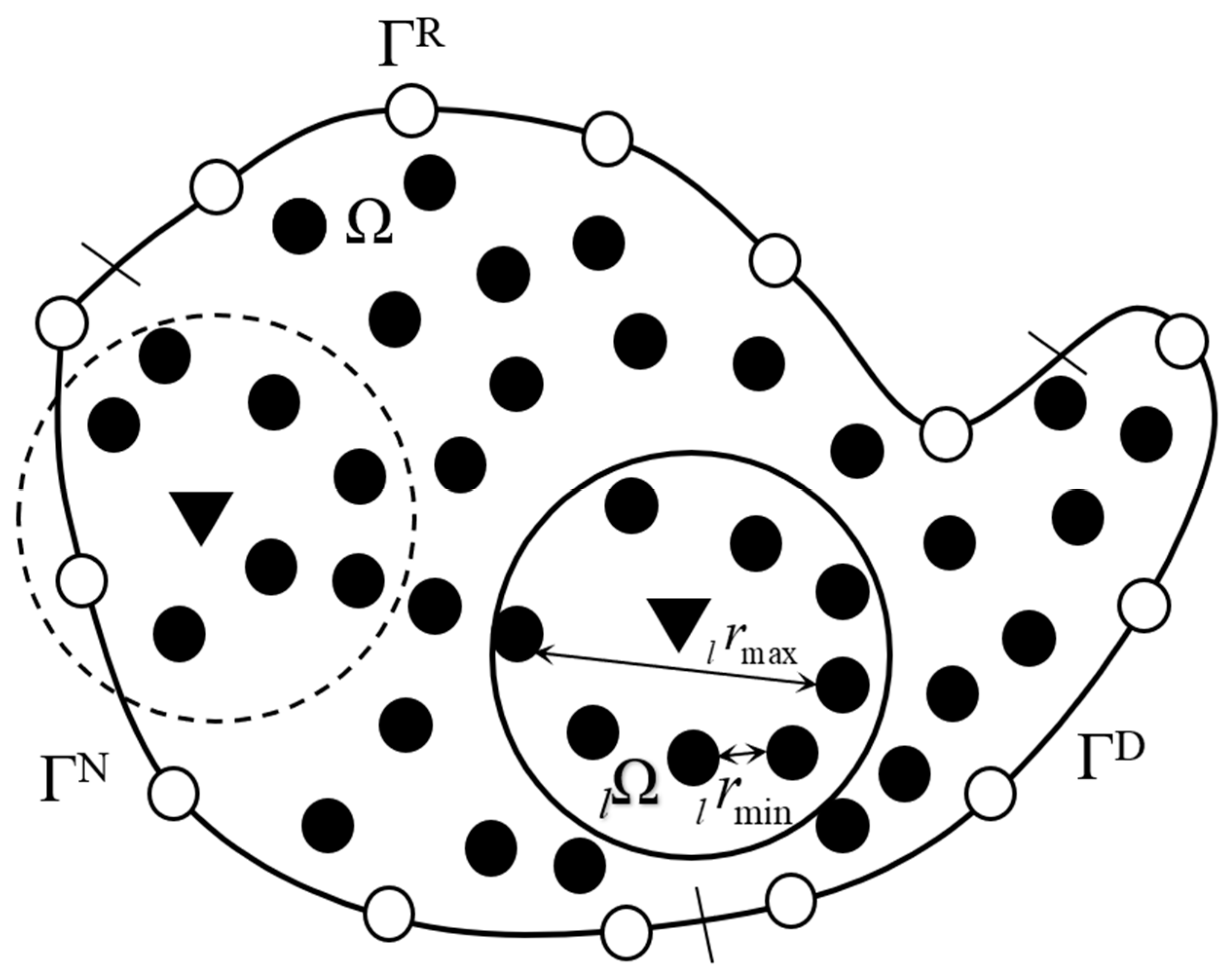
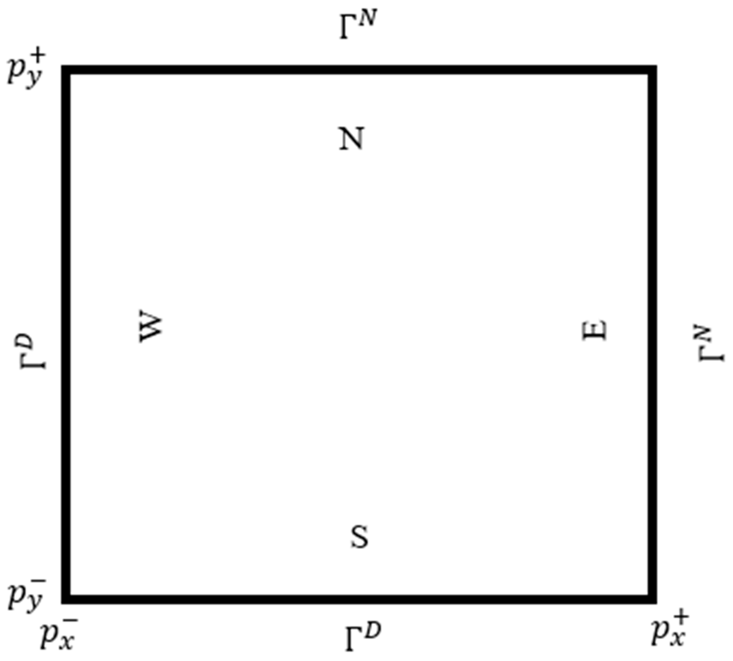
Figure 1.
Scheme of the domain Ω with boundary conditions weighted at ΓD, ΓR, and ΓN. The solid and empty circles show the interior and boundary nodes, respectively. The solid circular line shows the limits of the local sub-domain lΩ containing nine interior nodes. In contrast, a dashed circular line represents another local sub-domain, containing a boundary node and eight interior nodes, whereas the solid triangle shows the central node. and are the maximum and minimum distance between any node in the subdomain , respectively.
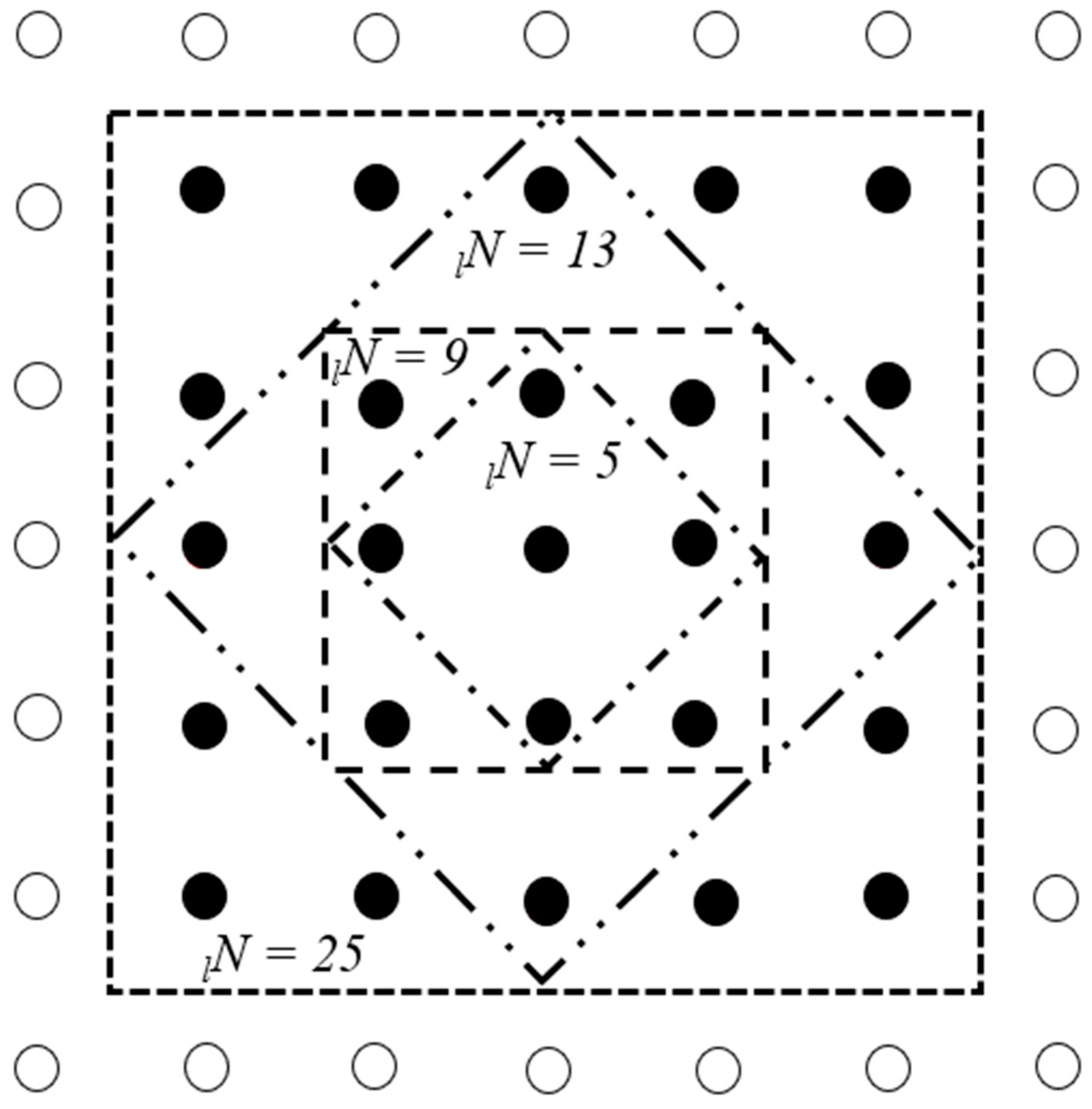
Figure 2.
Local sub-domain scheme for RND with . Solid and empty circles denote the inner and boundary nodes, respectively.
Figure 2.
Local sub-domain scheme for RND with . Solid and empty circles denote the inner and boundary nodes, respectively.
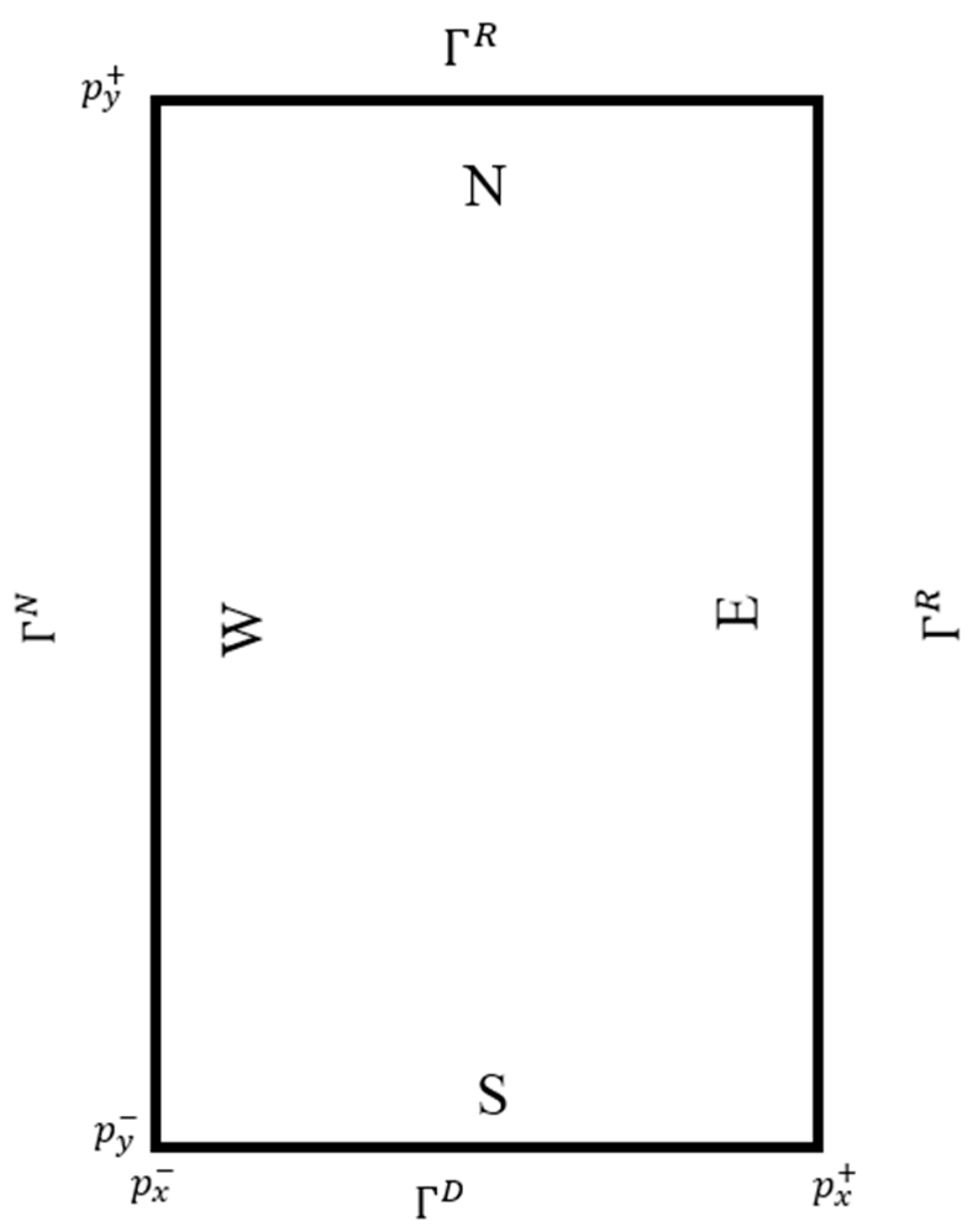
Figure 3.
Scheme of Case 1 with geometry () and boundary conditions.
Figure 3.
Scheme of Case 1 with geometry () and boundary conditions.
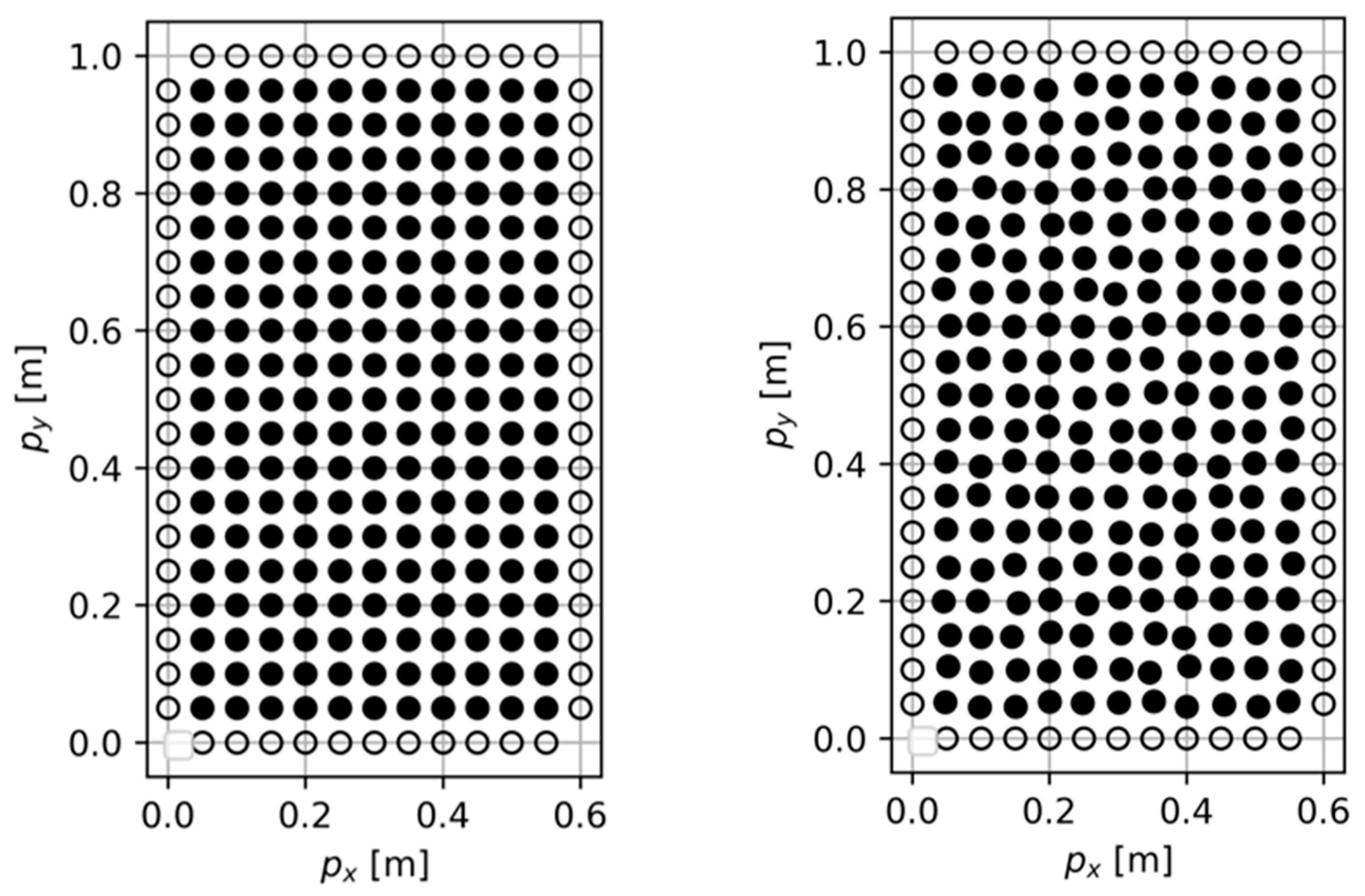
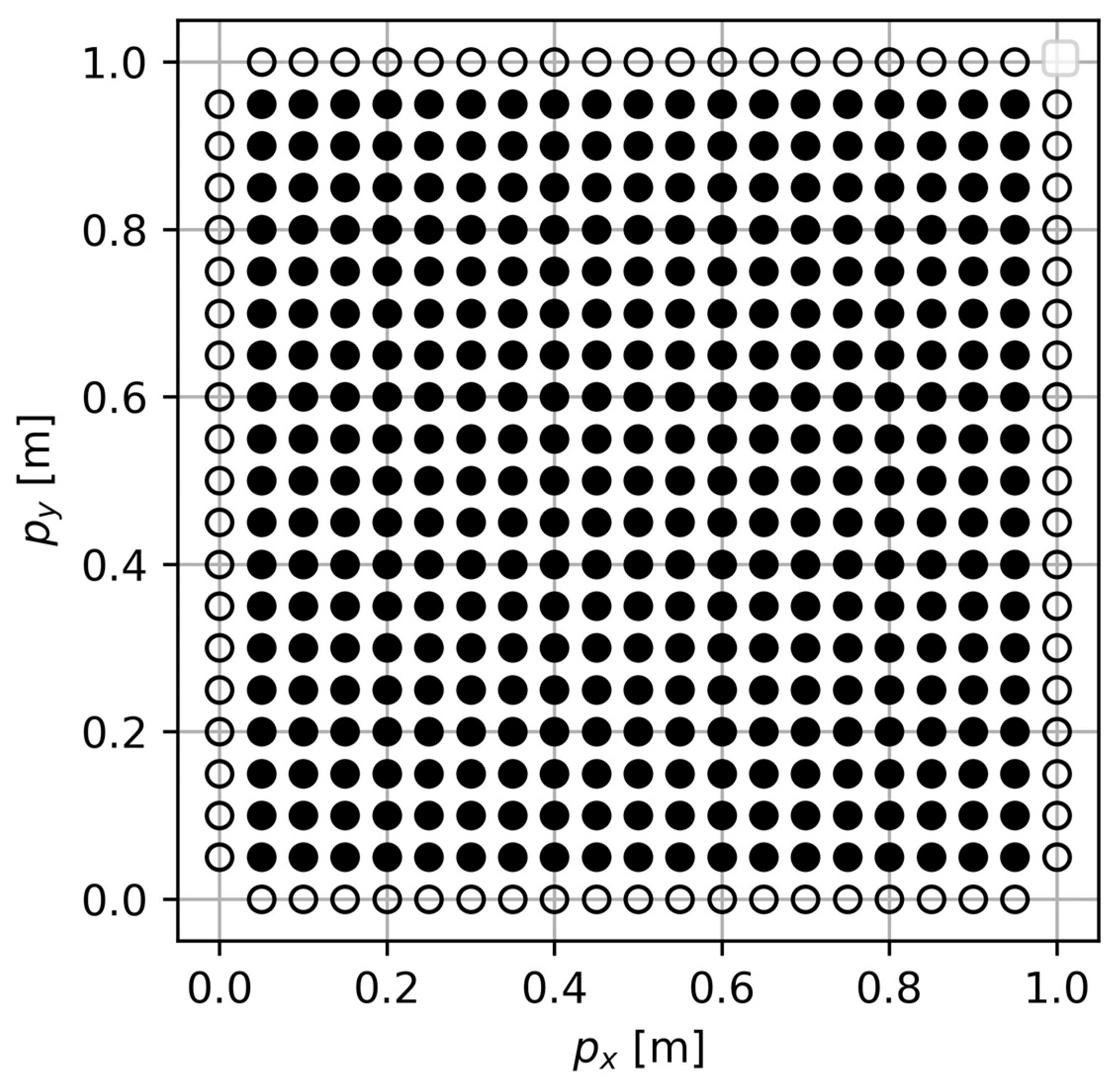
Figure 4.
Case 1, RND and QUND with nodes. In regular node distribution, the is 0.05 m and is 0.1802 m, while for QUND, is 0.0994 m, and the is 0.1839 m.
Figure 4.
Case 1, RND and QUND with nodes. In regular node distribution, the is 0.05 m and is 0.1802 m, while for QUND, is 0.0994 m, and the is 0.1839 m.
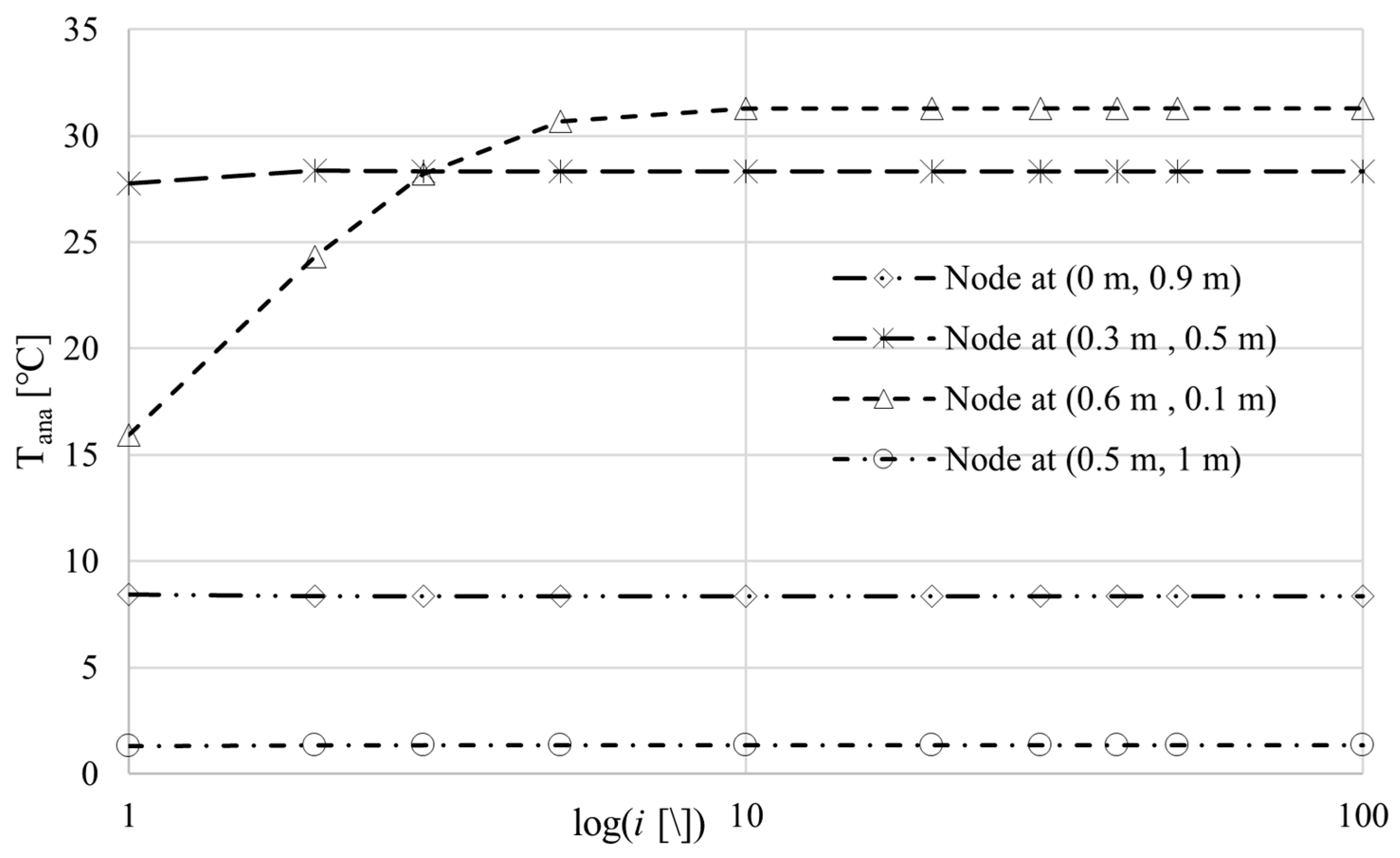
Figure 5.
Case 1, convergence analysis of analytical solution as a function of the terms used in the evaluation of Equation (33) for four different nodes, i.e., (0.6 m, 0.1 m), (0.5 m, 1 m), (0.3 m, 0.5 m), and (0 m, 0.9 m) of the rectangular geometry.
Figure 5.
Case 1, convergence analysis of analytical solution as a function of the terms used in the evaluation of Equation (33) for four different nodes, i.e., (0.6 m, 0.1 m), (0.5 m, 1 m), (0.3 m, 0.5 m), and (0 m, 0.9 m) of the rectangular geometry.
Figure 6.
Scheme of Case 2 with geometry () and boundary conditions.
Figure 6.
Scheme of Case 2 with geometry () and boundary conditions.
Figure 7.
Case 2, regular nodes distribution is shown for and node arrangement with is 0.05 m and is 0.18027 m, solid and empty circles representing the inner and boundary nodes respectively.
Figure 7.
Case 2, regular nodes distribution is shown for and node arrangement with is 0.05 m and is 0.18027 m, solid and empty circles representing the inner and boundary nodes respectively.
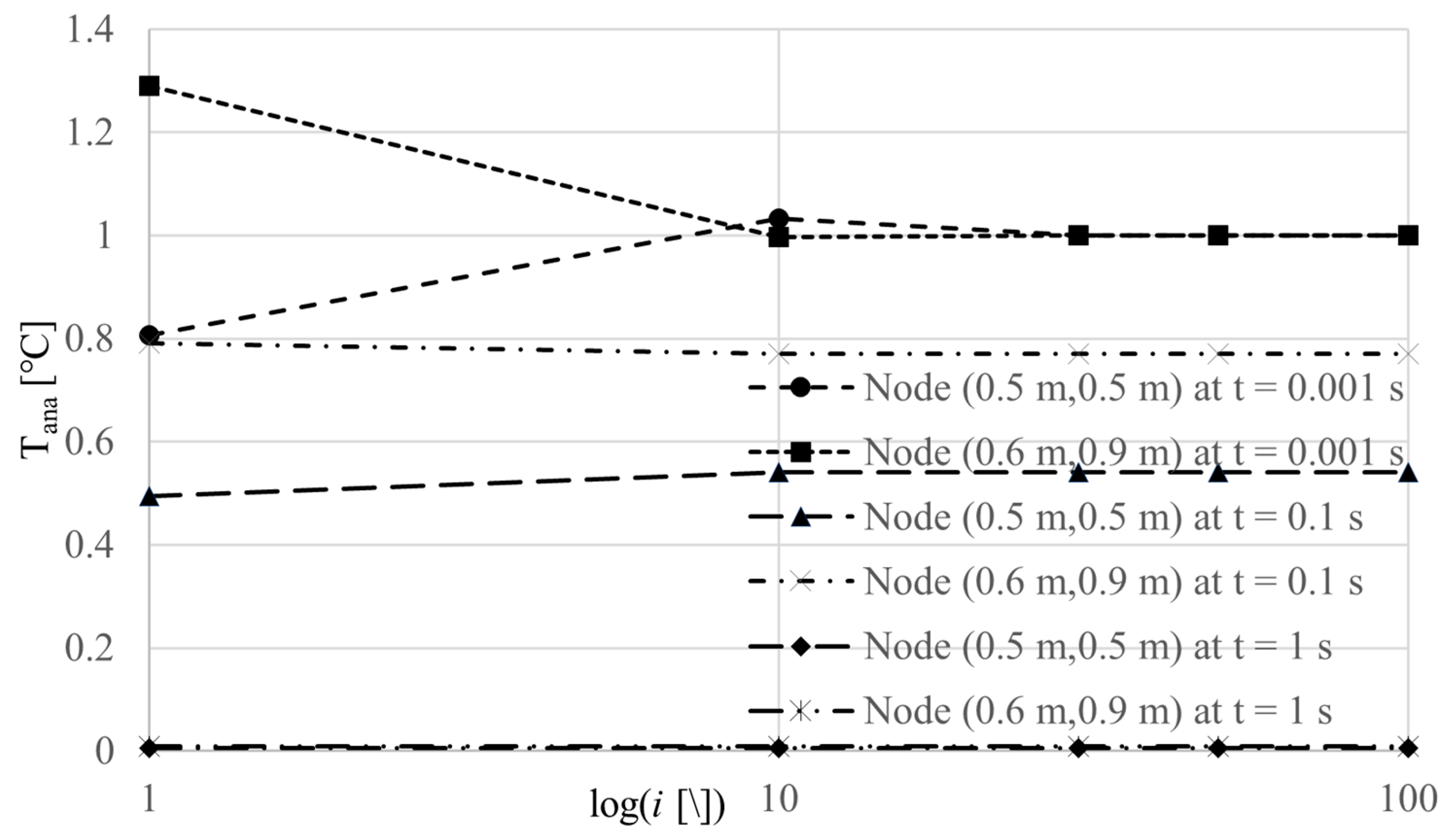
Figure 8.
Case 2, convergence analysis of analytical solution as a function of the terms used in evaluating Equation (39) for two nodes, i.e., at (0.5 m, 0.5 m) and (0.6 m, 0.9 m), of the square geometry for time t = 0.001 s, 0.1 s, and 1 s.
Figure 8.
Case 2, convergence analysis of analytical solution as a function of the terms used in evaluating Equation (39) for two nodes, i.e., at (0.5 m, 0.5 m) and (0.6 m, 0.9 m), of the square geometry for time t = 0.001 s, 0.1 s, and 1 s.
Figure 9.
Case 1, the difference in % of the as a function of the node distance for MQ with and without augmentation (RND, c = 64, ).
Figure 9.
Case 1, the difference in % of the as a function of the node distance for MQ with and without augmentation (RND, c = 64, ).
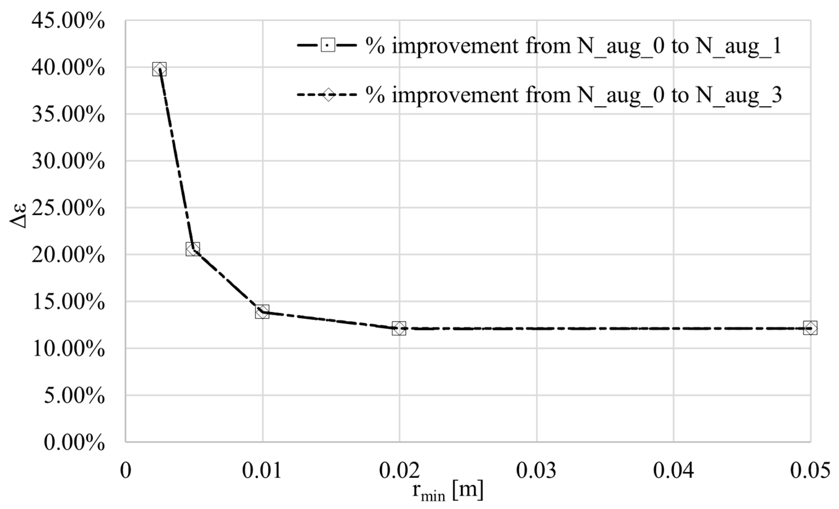
Figure 10.
Case 1, improvement in % of the as a function of the node distance for MQ with and without augmentation (RND, c = 64, ).
Figure 10.
Case 1, improvement in % of the as a function of the node distance for MQ with and without augmentation (RND, c = 64, ).
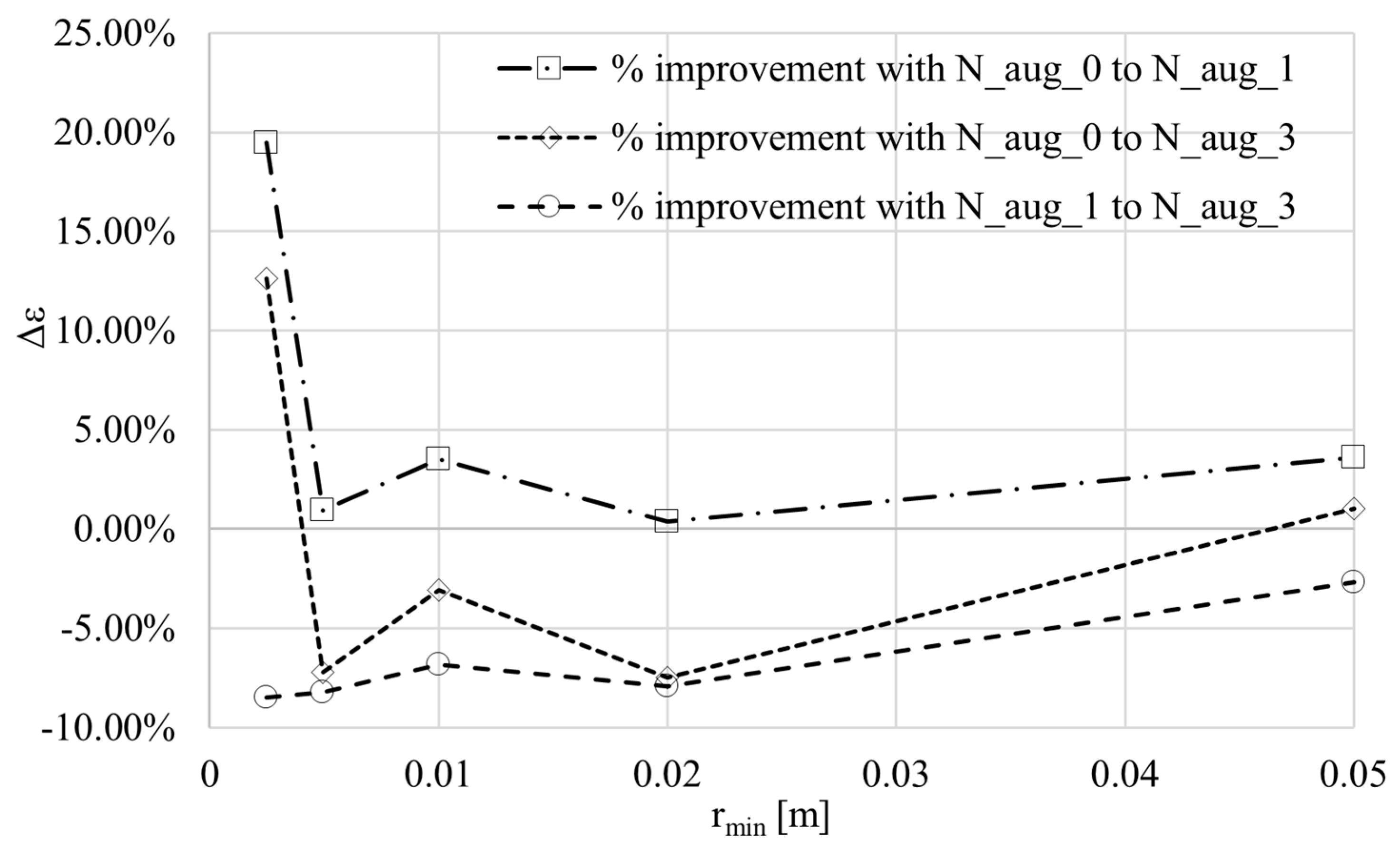
Figure 11.
Case 1, improvement in % of the as a function of the node distance for MQ with and without augmentation (RND, c = 32, ).
Figure 11.
Case 1, improvement in % of the as a function of the node distance for MQ with and without augmentation (RND, c = 32, ).
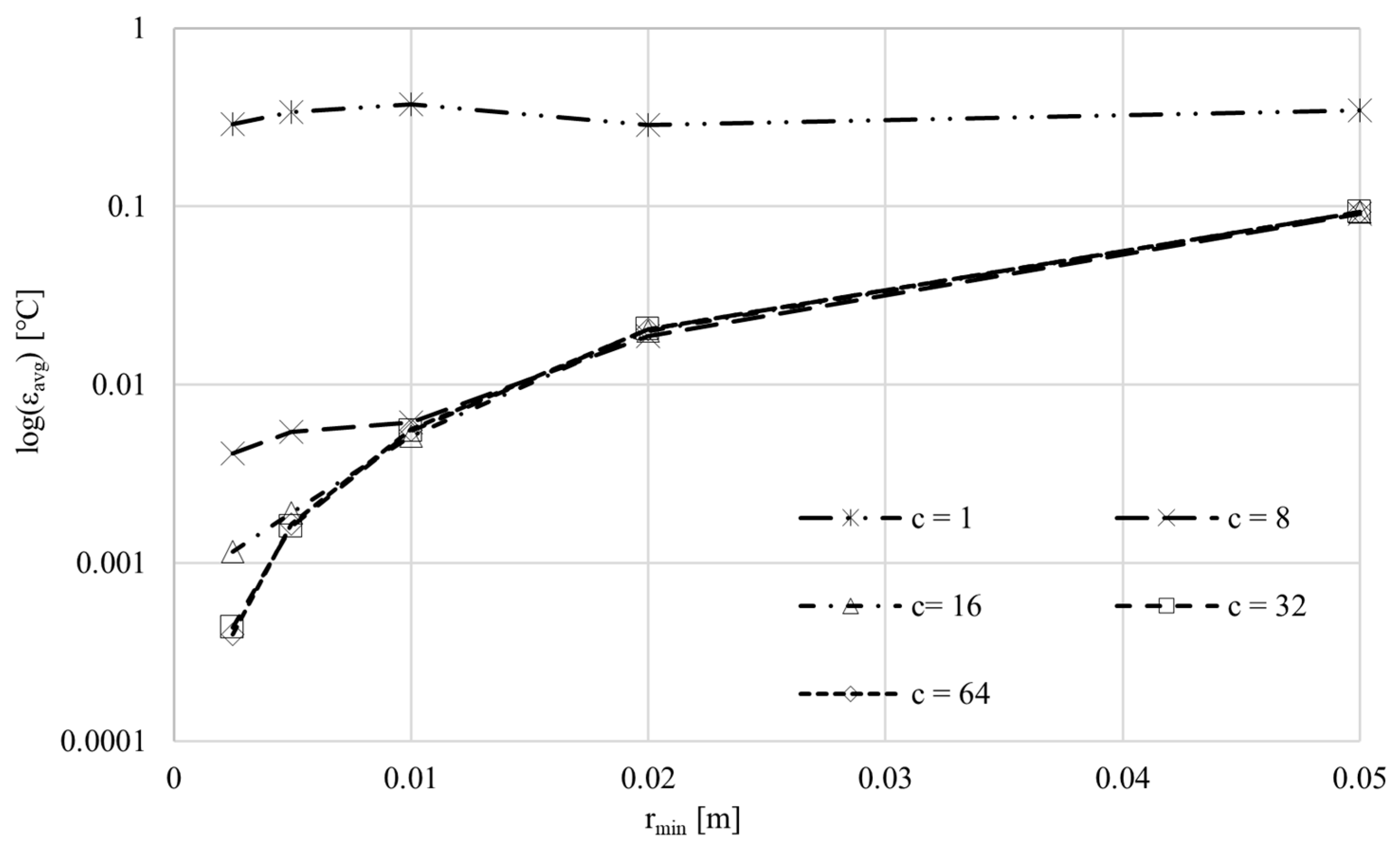
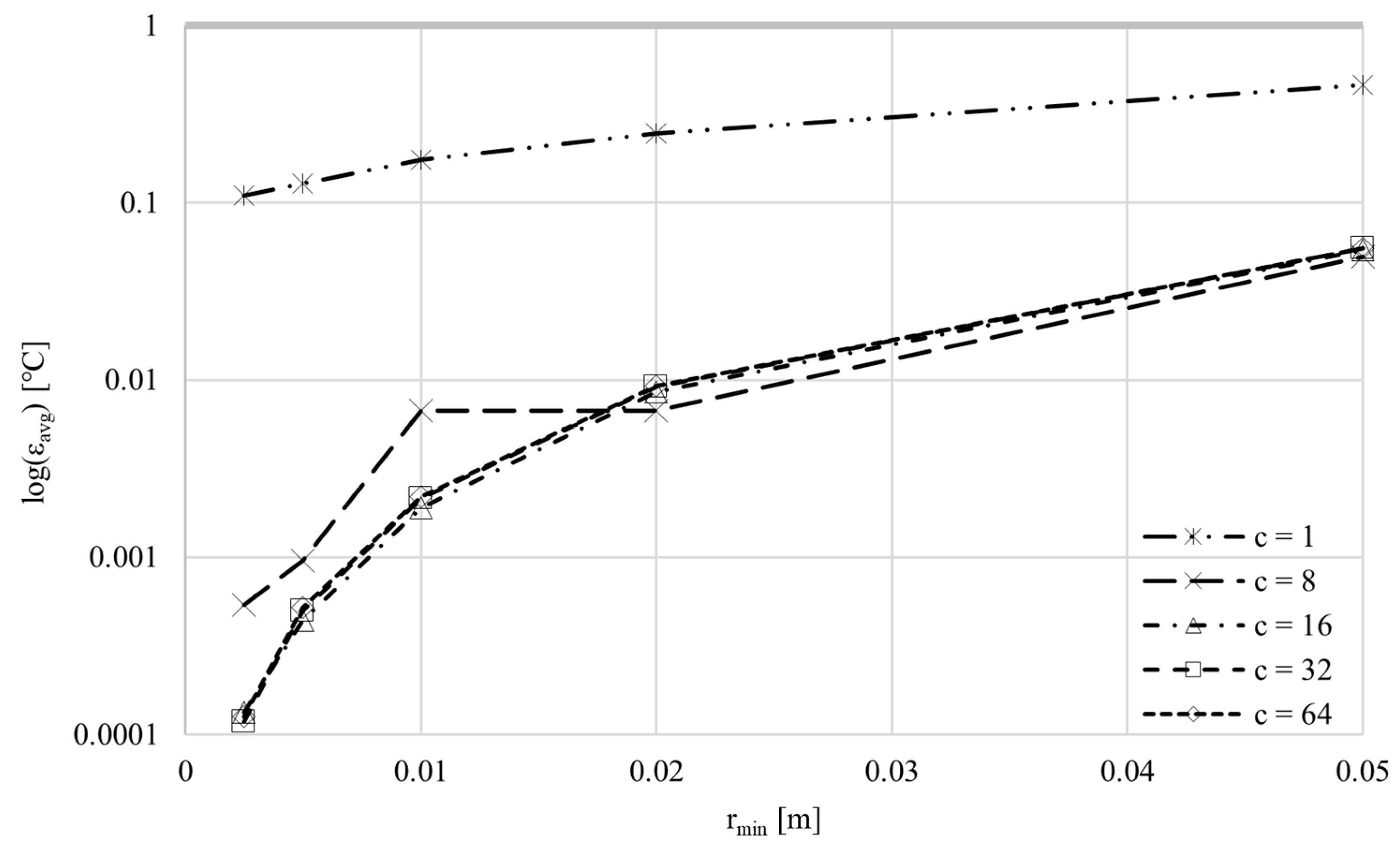
Figure 12.
Case 1, MQ, as a function of node distance calculated for five different shape pa-rameters (RND, , ).
Figure 12.
Case 1, MQ, as a function of node distance calculated for five different shape pa-rameters (RND, , ).
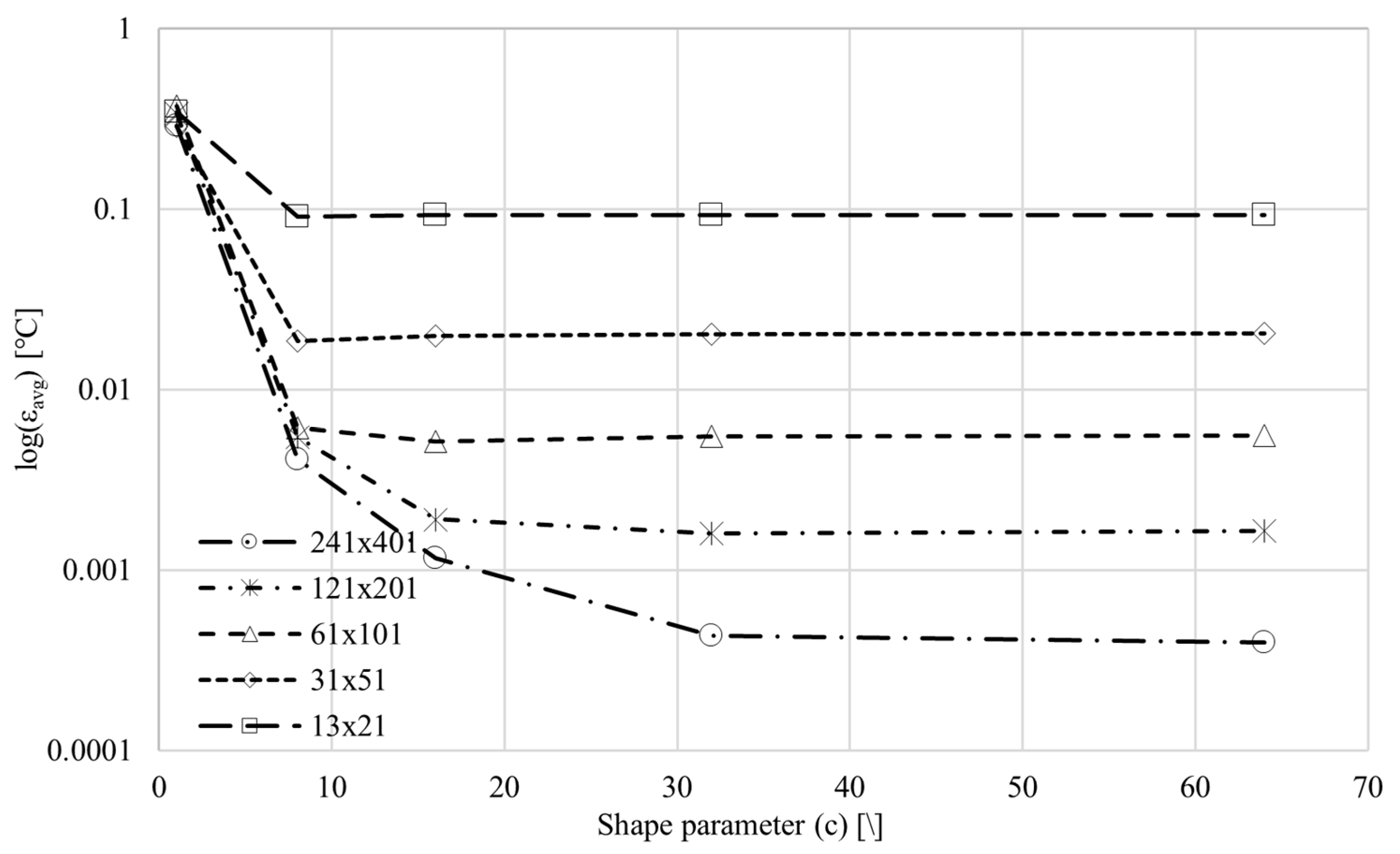
Figure 13.
Case 1, MQ, as a function of shape parameter (RND, , ).
Figure 13.
Case 1, MQ, as a function of shape parameter (RND, , ).
Figure 14.
Case 1, MQ, as a function of the node distance for different shape parameters (RND, , ).
Figure 14.
Case 1, MQ, as a function of the node distance for different shape parameters (RND, , ).
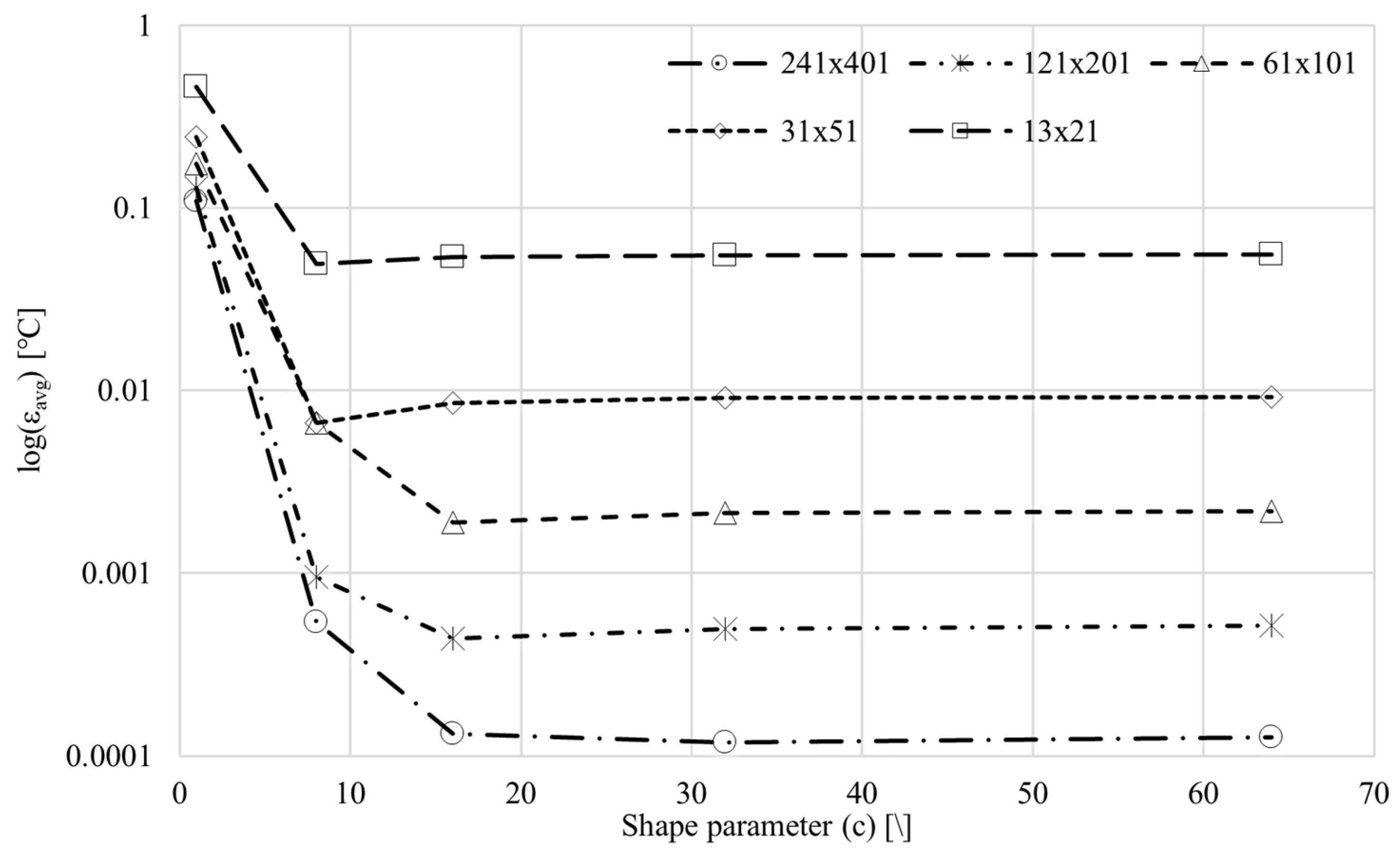
Figure 15.
Case 1, MQ, as a function of the shape parameter (RND, , ).
Figure 15.
Case 1, MQ, as a function of the shape parameter (RND, , ).
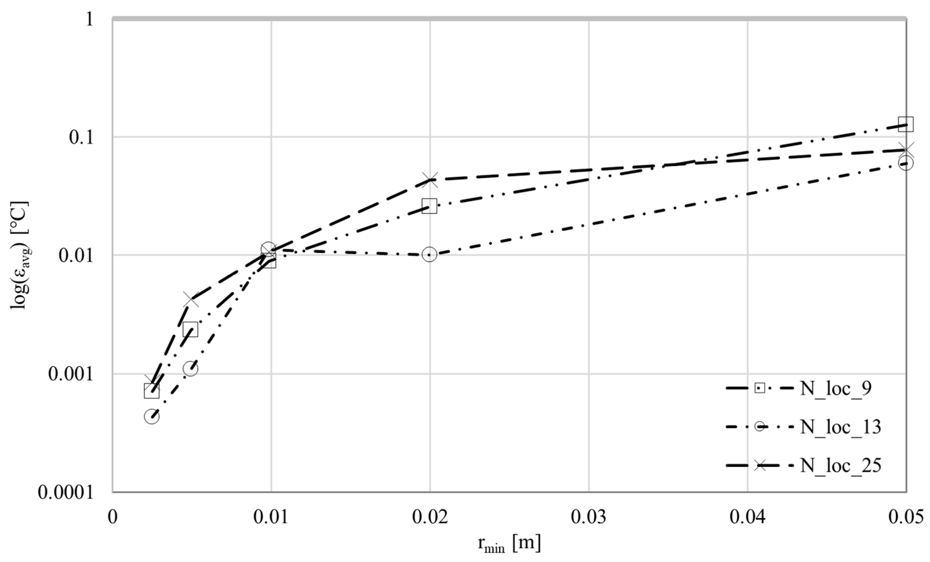
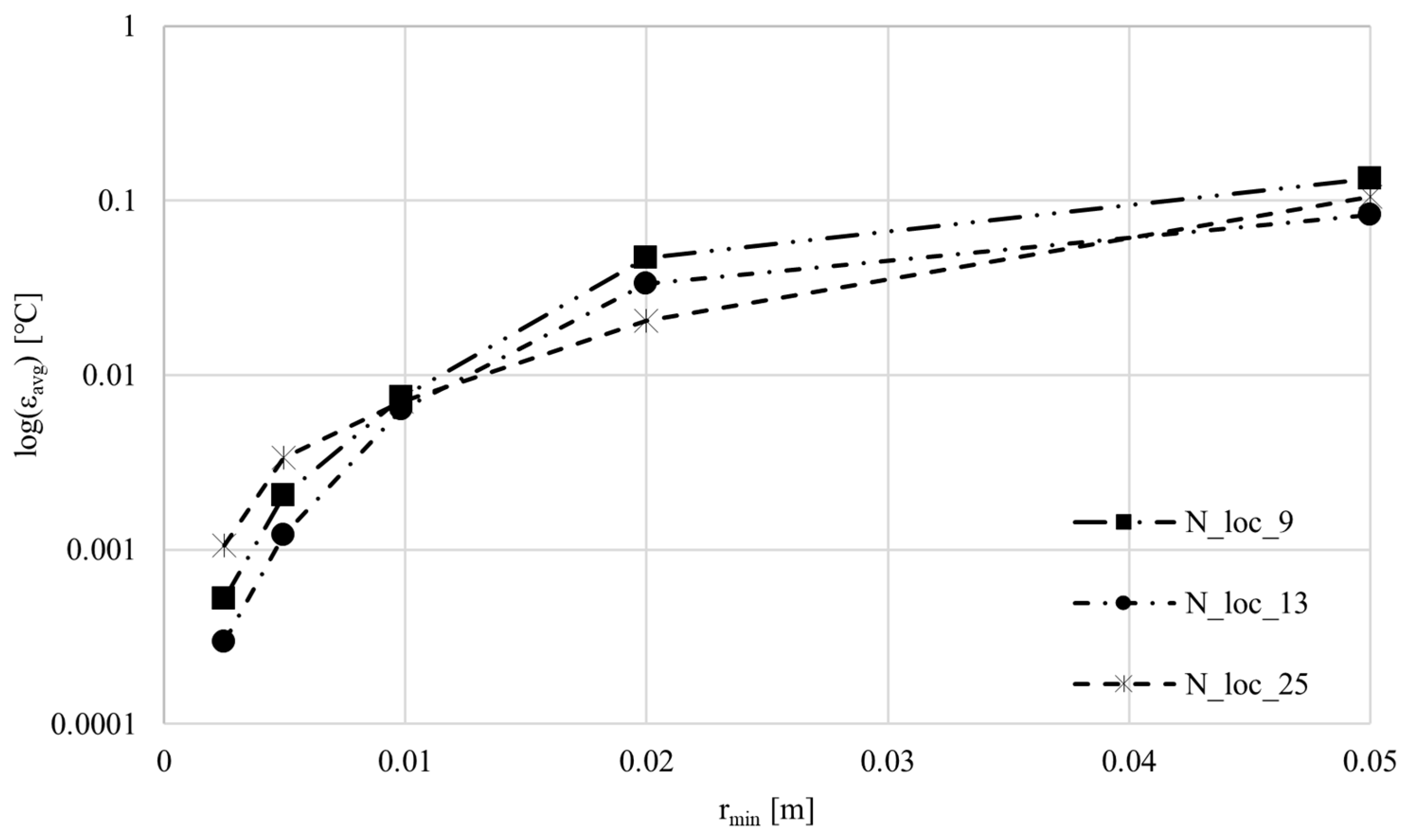
Figure 16.
Case 1, PHS, as a function of node distance for a different number of nodes in the local subdomain (RND, ).
Figure 16.
Case 1, PHS, as a function of node distance for a different number of nodes in the local subdomain (RND, ).
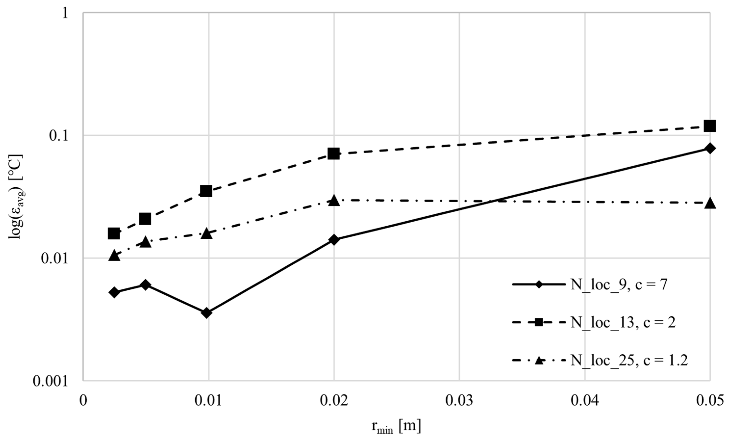
Figure 17.
Case 1, MQ, as a function node distance with a different number of nodes in the local subdomain and optimum shape parameter (RND, ).
Figure 17.
Case 1, MQ, as a function node distance with a different number of nodes in the local subdomain and optimum shape parameter (RND, ).
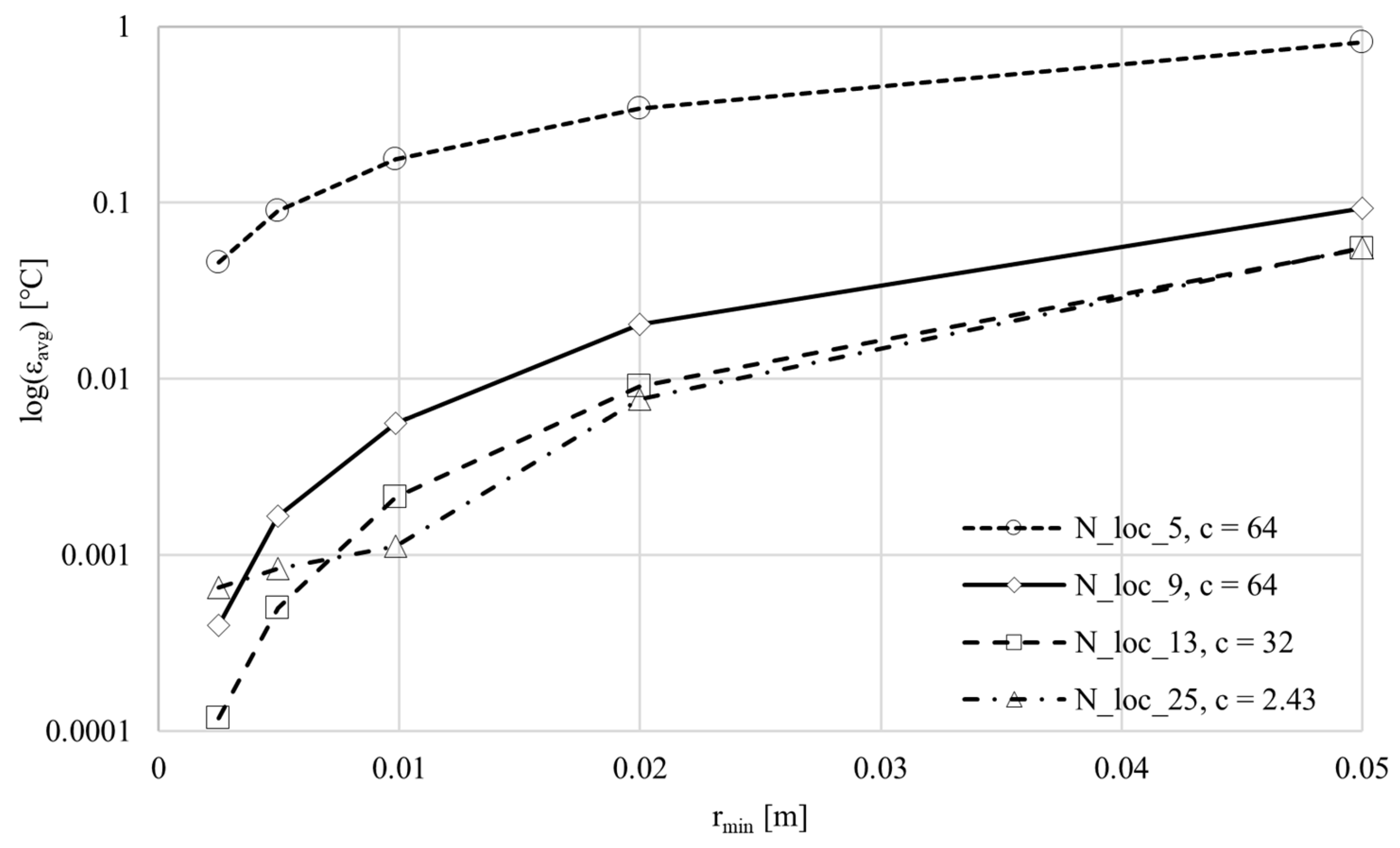
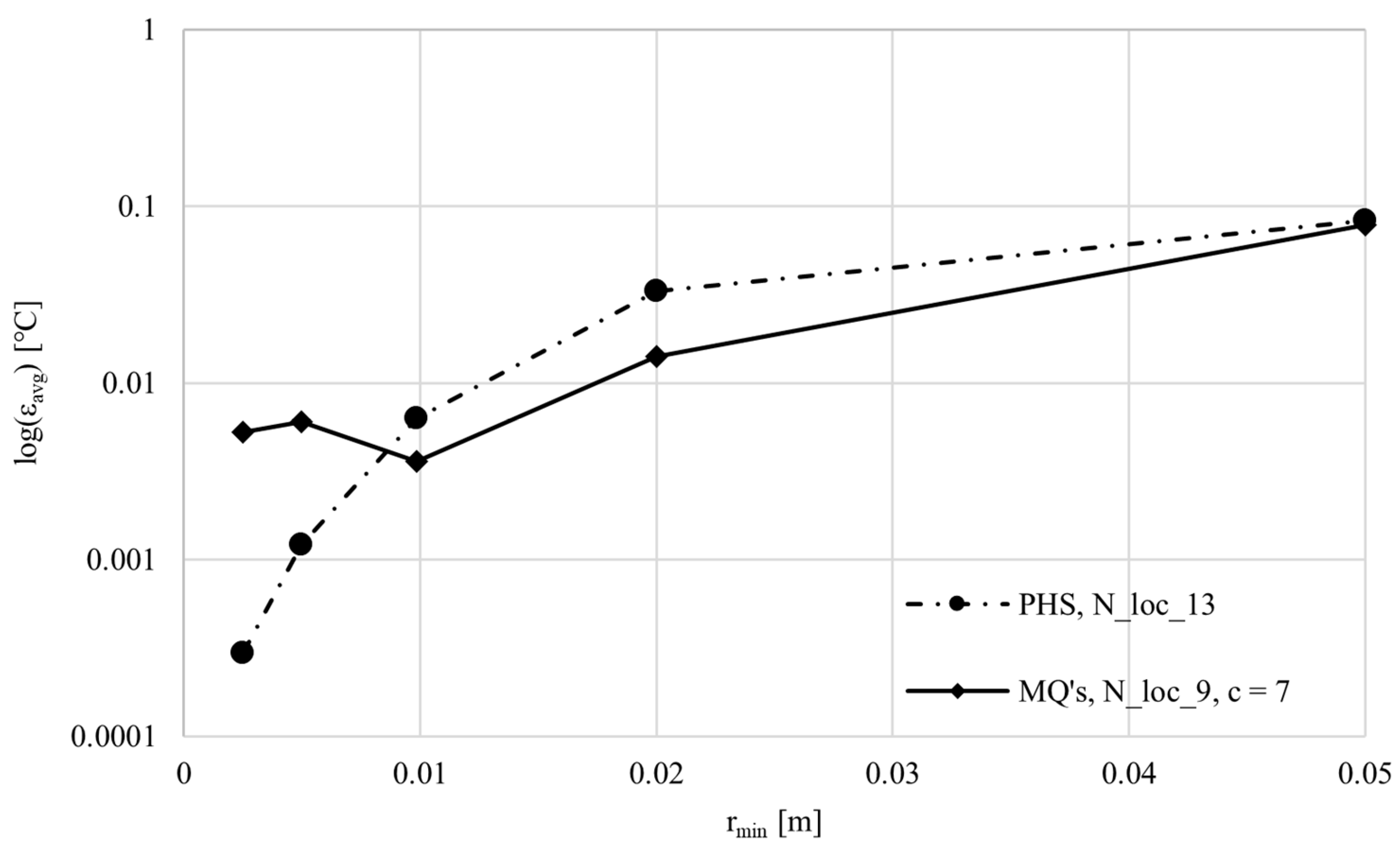
Figure 18.
Case 1, as a function of node distance (RND, MQ with , and PHS with ).
Figure 18.
Case 1, as a function of node distance (RND, MQ with , and PHS with ).
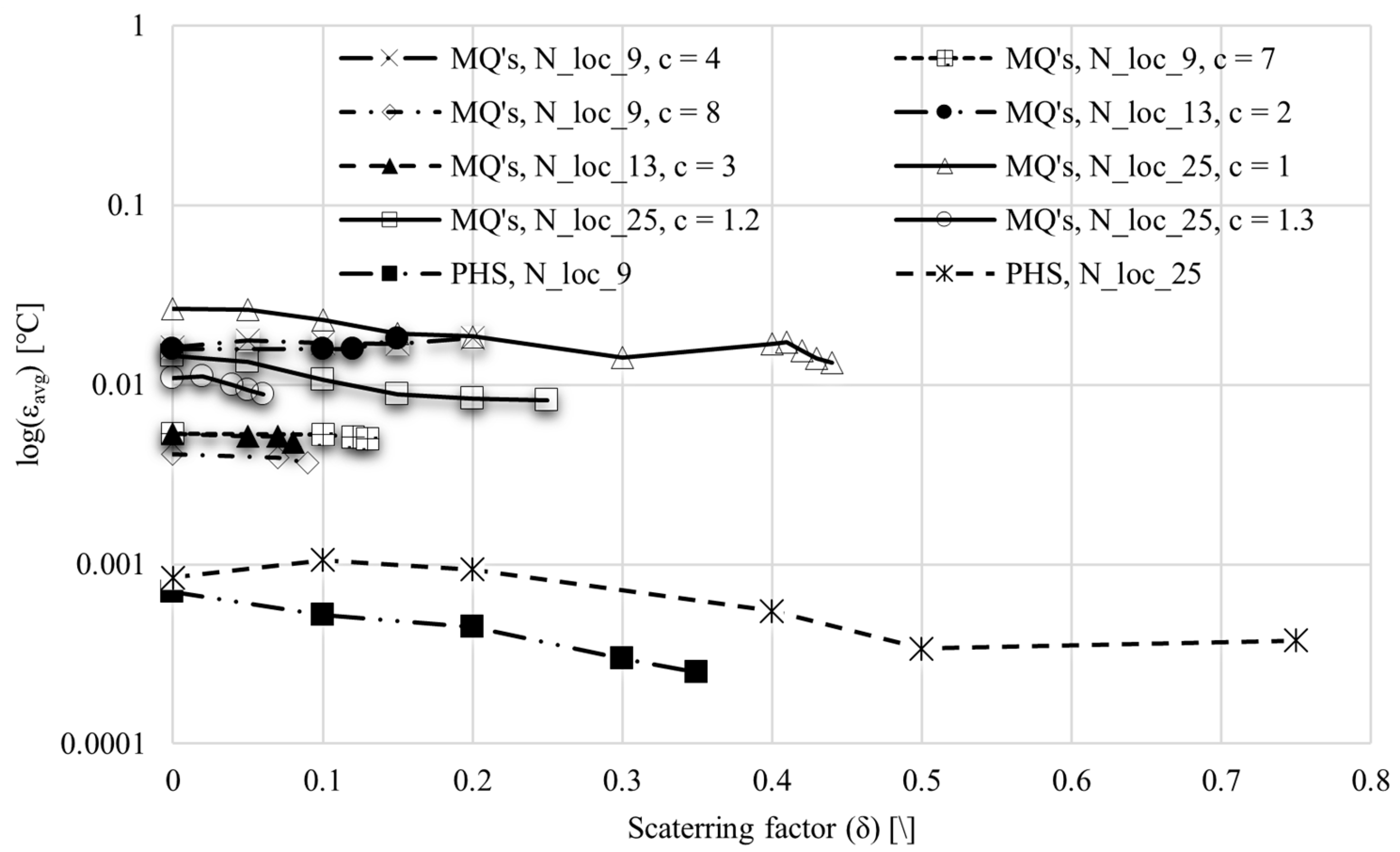
Figure 19.
Case 1, as a function of the scattering factor () (QUND, ).
Figure 19.
Case 1, as a function of the scattering factor () (QUND, ).
Figure 20.
Case 1, PHS, error as a function of the node distance for different (QUND, , ).
Figure 20.
Case 1, PHS, error as a function of the node distance for different (QUND, , ).
Figure 21.
Case 1, MQ, as a function of the node distance for different (QUND, ).
Figure 21.
Case 1, MQ, as a function of the node distance for different (QUND, ).
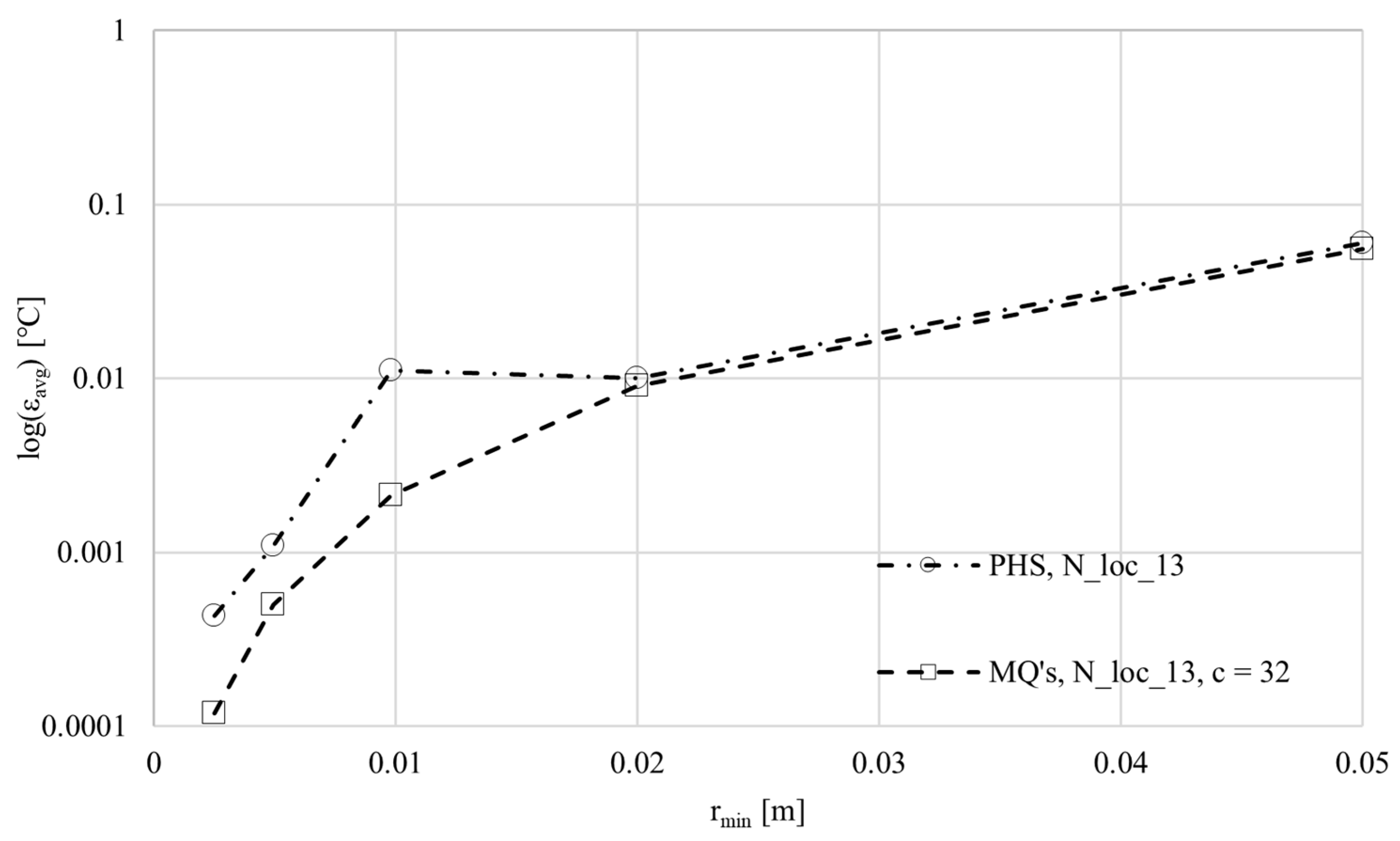
Figure 22.
Case 1, as a function of node distance (QUND, , MQ with , PHS with ).
Figure 22.
Case 1, as a function of node distance (QUND, , MQ with , PHS with ).
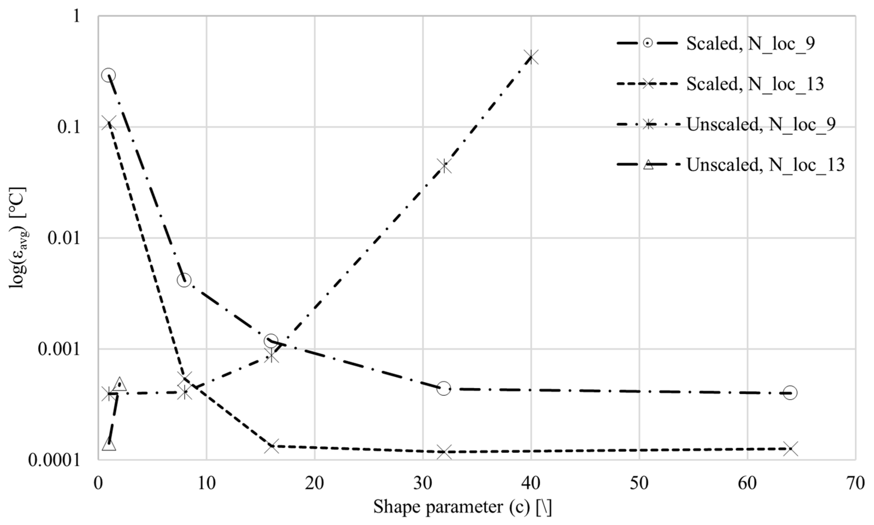
Figure 23.
Case 1, as a function of the shape parameter (c) for scaled and unscaled MQs (RND, ).
Figure 23.
Case 1, as a function of the shape parameter (c) for scaled and unscaled MQs (RND, ).
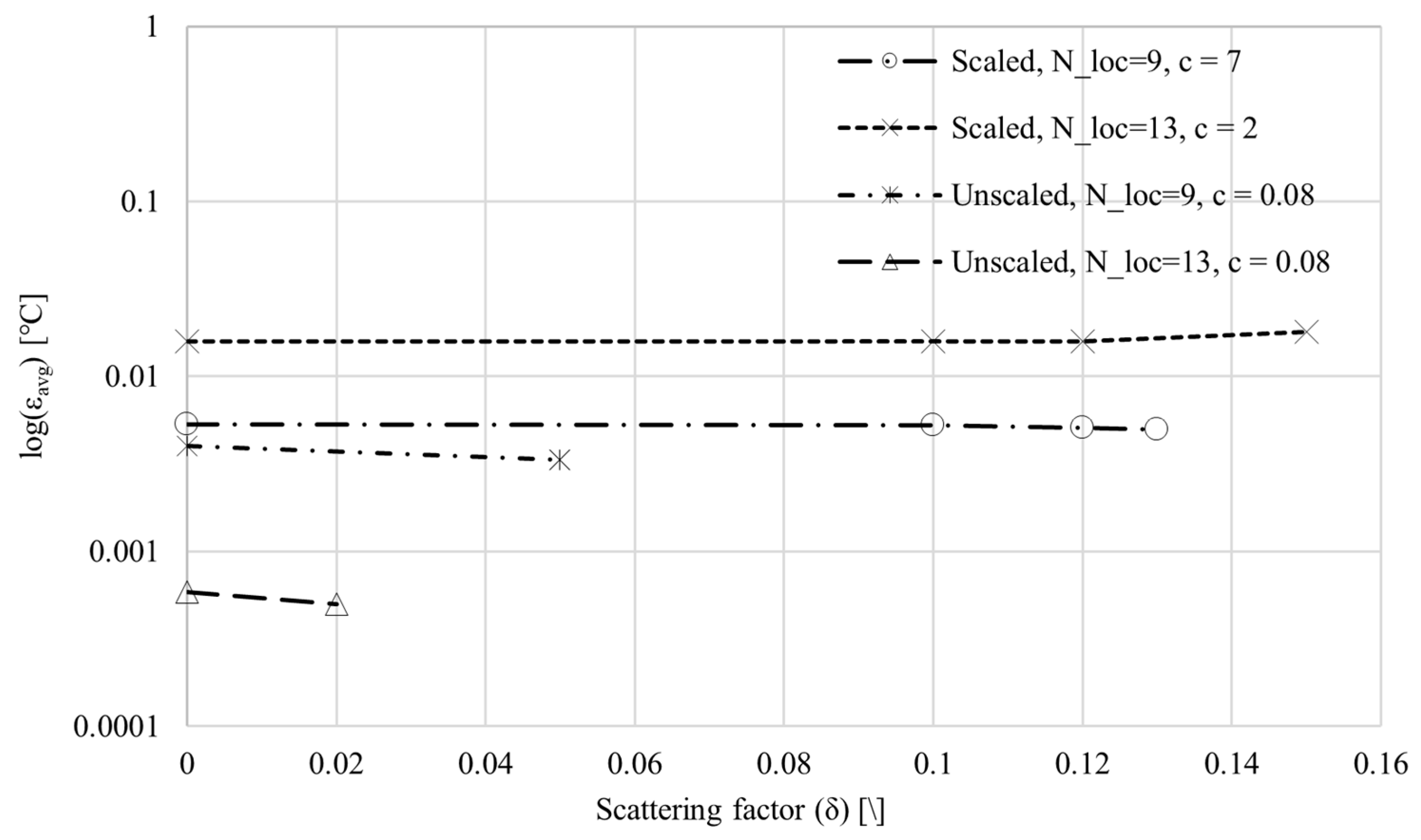
Figure 24.
Case 1, as a function of the scattering factor () for scaled and unscaled MQs (QUND, ).
Figure 24.
Case 1, as a function of the scattering factor () for scaled and unscaled MQs (QUND, ).
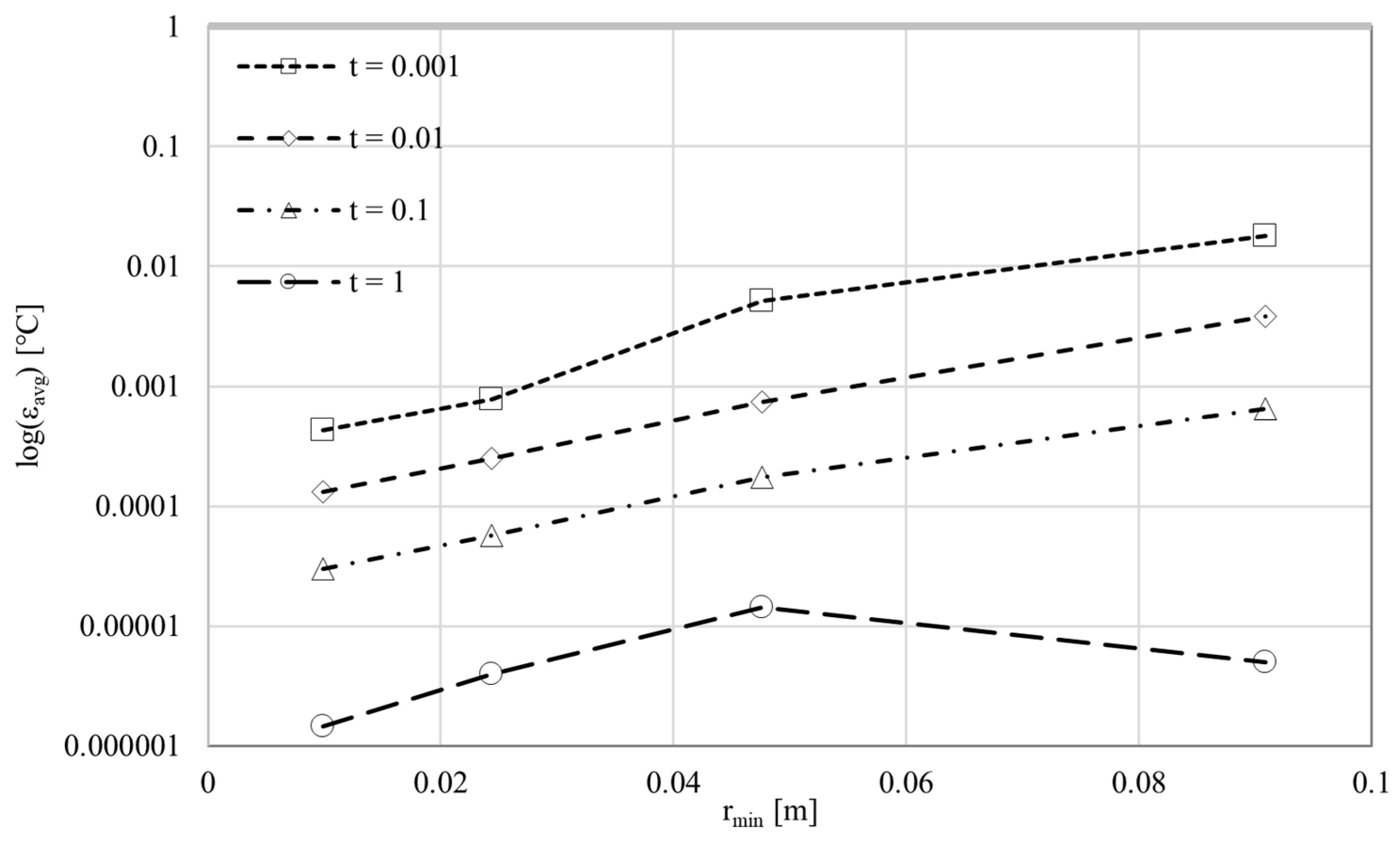
Figure 25.
Case 2, MQ, as a function of node distance for four different times (RND, , , c = 32).
Figure 25.
Case 2, MQ, as a function of node distance for four different times (RND, , , c = 32).
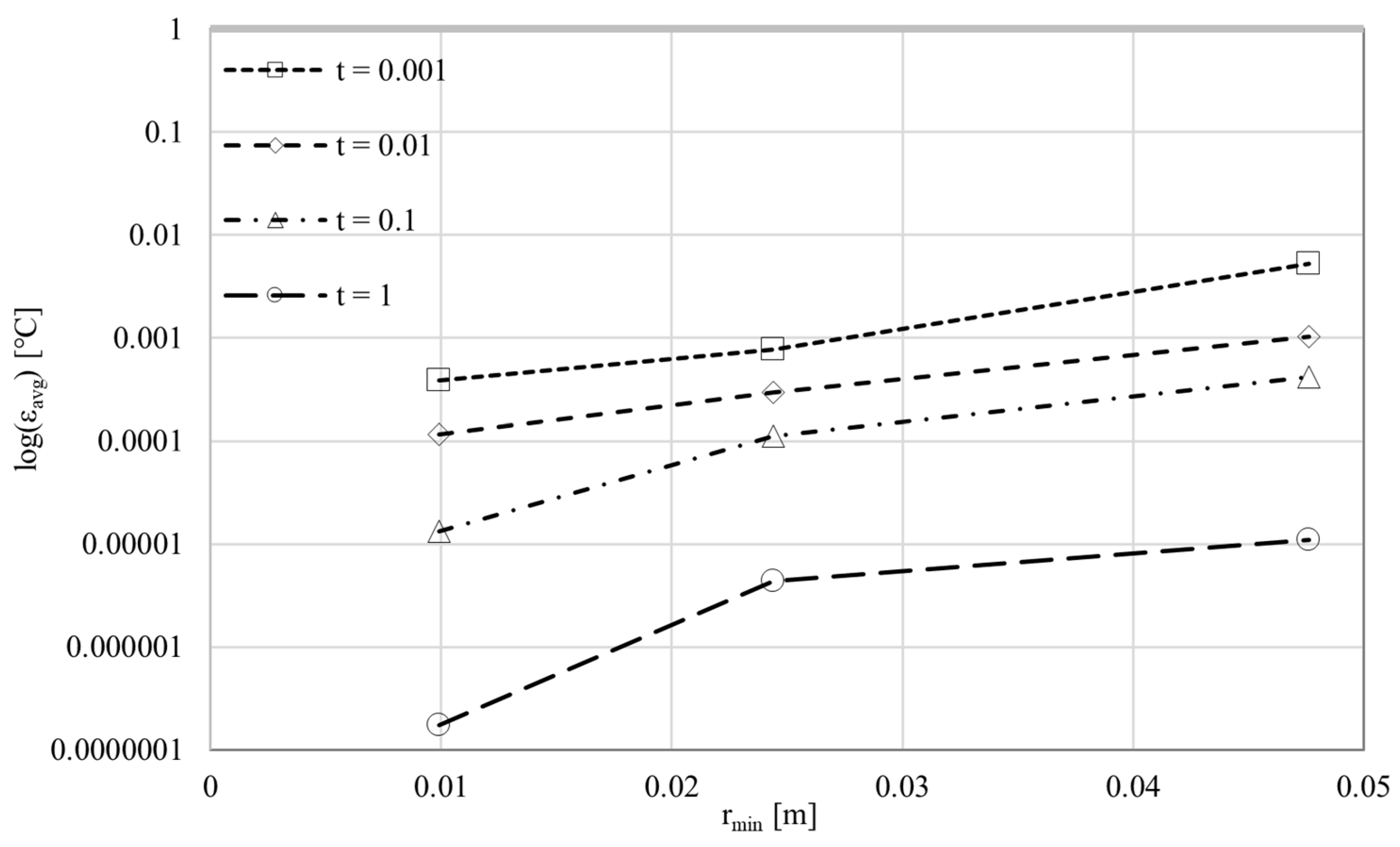
Figure 26.
Case 2, MQ, as a function of node distance for three different (RND, , c = 32, t = 1 s).
Figure 26.
Case 2, MQ, as a function of node distance for three different (RND, , c = 32, t = 1 s).
Figure 27.
Case 2, MQ, as a function of node distance for four different with optimal shape parameters (RND, , t = 1 s).
Figure 27.
Case 2, MQ, as a function of node distance for four different with optimal shape parameters (RND, , t = 1 s).
Figure 28.
Case 2, PHS, as a function of node distance for four different times (RND, , ).
Figure 28.
Case 2, PHS, as a function of node distance for four different times (RND, , ).
Figure 29.
Case 2, PHS, as a function of node distance for four different times (RND, , ).
Figure 29.
Case 2, PHS, as a function of node distance for four different times (RND, , ).
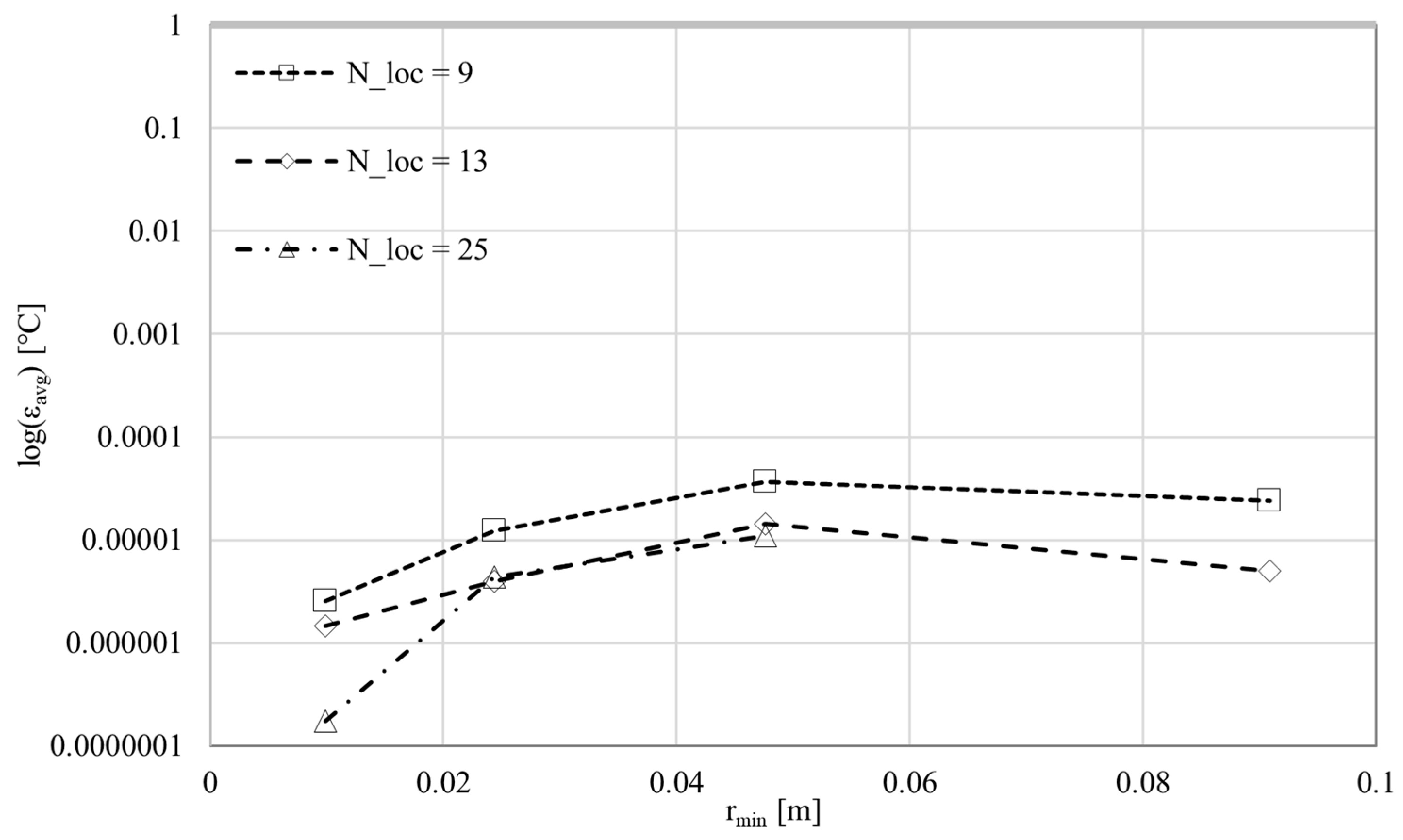
Figure 30.
Case 2, PHS, as a function of node distance for four different times and three node arrangements (RND, , ).
Figure 30.
Case 2, PHS, as a function of node distance for four different times and three node arrangements (RND, , ).
Figure 31.
Case 2, PHS, as a function of node distance for three different (RND, , t = 1 s,).
Figure 31.
Case 2, PHS, as a function of node distance for three different (RND, , t = 1 s,).
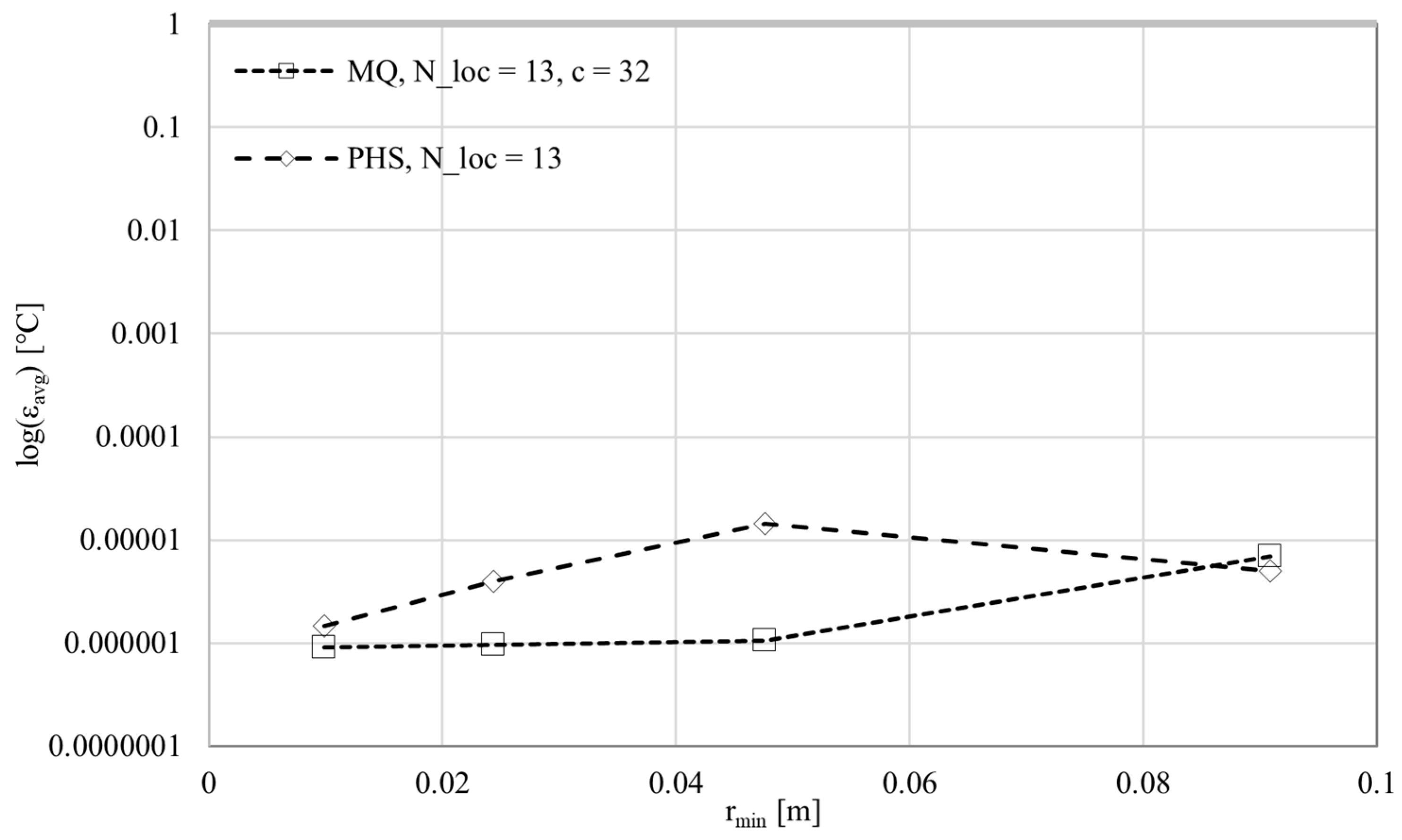
Figure 32.
Case 2, comparison of MQ () and PHS () in terms of as a function of node distance (RND, , t = 1 s).
Figure 32.
Case 2, comparison of MQ () and PHS () in terms of as a function of node distance (RND, , t = 1 s).
Table 1.
Material properties, boundary, and initial conditions used in Case 1 studies.
Table 1.
Material properties, boundary, and initial conditions used in Case 1 studies.
| Material Property | Value |
|---|
| Density (ρ) [kg/m3] | 7850 |
| Specific heat I [J/(kg K)] | 460 |
| Thermal conductivity (k) [W/(mK)] | 52 |
| Heat transfer coefficient (h) [W/(m2K)] | 750 |
| Reference temperature () [°C] | 0 |
| Dirichlet boundary temperature () [°C] | 100 |
| Neuman boundary condition () [W/m2] | 0 |
Table 2.
Fixed parameters used in the simulations of Case 1 studies.
Table 2.
Fixed parameters used in the simulations of Case 1 studies.
| RBF | PHS | MQ |
|---|
| Δt [s] | 0.005 | 0.005 |
| 9 | 9 |
| 13 | 13 |
| 25 | 25 |
| c | - | 1 |
| - | 8 |
| - | 16 |
| - | 32 |
| - | 64 |
| 6 | 1 |
| Scattering factor () | 0.10 | 0.10 |
| [°C] | 10−6 | 10−6 |
| Initial temperature () [°C] | 100 | 100 |
Table 3.
Node densities with boundary and domain nodes used in Case 1 studies.
Table 3.
Node densities with boundary and domain nodes used in Case 1 studies.
| Node’s Arrangement | Total Number of Nodes ( | | ) |
|---|
| 13 × 21 | 269 | 60 | 209 |
| 31 × 51 | 1577 | 156 | 1421 |
| 61 × 101 | 6157 | 316 | 5841 |
| 121 × 201 | 24,321 | 636 | 23,685 |
| 241 × 401 | 96,641 | 1276 | 95,365 |
Table 4.
Minimum and used mesh Fourier number for the stable solution of Case 1.
Table 4.
Minimum and used mesh Fourier number for the stable solution of Case 1.
| | | [m] |
|---|
| 241 × 401 | 0.25 | 0.116 | 0.002 |
| 121 × 201 | 0.25 | 0.029 | 0.005 |
| 61 × 101 | 0.25 | 0.00744 | 0.00984 |
| 31 × 51 | 0.25 | 0.00180 | 0.02000 |
| 13 × 21 | 0.25 | 0.00029 | 0.05000 |
Table 5.
Material properties used in Case 2 studies.
Table 5.
Material properties used in Case 2 studies.
| Material Property | Value |
|---|
| Density (ρ) [kg/m3] | 1 |
| Specific heat (c) [J/(kg K)] | 1 |
| Thermal conductivity (k) [W/(mK)] | 1 |
| Initial temperature () [°C] | 1 |
Table 6.
Fixed parameters used for the simulations in Case 2 studies.
Table 6.
Fixed parameters used for the simulations in Case 2 studies.
| RBF | PHS | MQ |
|---|
| Δt [s] | 10−6 | 10−6 |
| t [s] | 1 | 1 |
| 0.1 | 0.1 |
| 0.01 | 0.01 |
| 0.001 | 0.001 |
| - | 5 |
| 9 | 9 |
| 13 | 13 |
| 25 | 25 |
| c | - | 8 |
| - | 16 |
| - | 32 |
| - | 64 |
| 6 | 1 |
Table 7.
Node densities with boundary and domain nodes used in Case 2 studies.
Table 7.
Node densities with boundary and domain nodes used in Case 2 studies.
| Node’s Arrangement | Total Number of Nodes () | | |
|---|
| 11 × 11 | 117 | 32 | 85 |
| 21 × 21 | 437 | 72 | 365 |
| 41 × 41 | 1677 | 152 | 1525 |
| 101 × 101 | 10197 | 392 | 9805 |
Table 8.
Minimum and used mesh Fourier number for the stable solution of Case 2.
Table 8.
Minimum and used mesh Fourier number for the stable solution of Case 2.
| | | [m] |
|---|
| 11 × 11 | 0.25 | 0.00121 | 0.09090 |
| 21 × 21 | 0.25 | 0.00441 | 0.04761 |
| 41 × 41 | 0.25 | 0.01681 | 0.02439 |
| 101 × 101 | 0.25 | 0.102 | 0.00990 |


