Applying Quaternions to Recognize Hidden Details in Images: Rothko as a Case Study

Abstract

Images or paintings with homogeneous colors may appear dull to the naked eye; however, there may be numerous details in the image that are expressed through subtle changes in color. This manuscript introduces a novel approach that can uncover these concealed details via a transformation that increases the distance between adjacent pixels, ultimately leading to a newly modified version of the input image. We chose the artworks of Mark Rothko—famous for their simplicity and limited color palette—as a case study. Our approach offers a different perspective, leading to the discovery of either accidental or deliberate clusters of colors. Our method is based on the quaternion ring, wherein a suitable multiplication can be used to boost the color difference between neighboring pixels, thereby unveiling new details in the image. The quality of the transformation between the original image and the resultant versions can be measured by the ratio between the number of connected components in the original image (m) and the number of connected components in the output versions (n), which usually satisfies $\frac{n}{m}\gg 1$. Although this procedure has been employed as a case study for artworks, it can be applied to any type of image with a similar simplicity and limited color palette.

1. Introduction

Our starting point for this research was a friendly discussion about Mark Rothko’s artworks [1], which are characterized by their simplicity and few colors. His simple-looking artworks led us to think about the possibility of finding hidden details within them, as well as in general.

This discussion made us consider the possibility of using various techniques to uncover hidden details in artworks. The intuitive approach is to explore such images using machine learning, deep learning, and general artificial intelligence, which unusually relies on methods of statistical inference. In [2], a convolutional neural network has been defined to generate artificial Rembrandt works based on his previous works. In [3], famous paintings are explored using K-means clustering, developing a system called artistic coloring, which automatically extracts the color characteristics of the artwork and applies them to color transfer.

In contrast, the conservative methods are based on ideas of real analysis and calculus, as in [4], which improves the grayscale by using affine transformations on a given image.

Rothko is a major figure in modern art, whose paintings are often distinguished by their simplicity and rectangles of solid colors. In our capacity as Rothko fans, we wondered if we might be able to reveal in Rothko’s paintings something he did not know about his own paintings or something he considered important but which the average image viewer did not observe (or simply a digitization error). The topic of revealing details in images has already been discussed in [5,6], where different image analysis approaches are provided to reveal invisible or hardly discernible details in art and manuscripts based on blind source separation or linear discriminant analysis.

In some cases, with the right procedure, an area within the image can represent two different objects, as in [7], images in which one or more secondary objects (or scenes) are hidden within a primary image. A system was presented for creating such images using a modified Poisson blending, which detects the edges of the object to be hidden, and then finds a place where it can be embedded within the scene, together with a suitable transformation.

In [8], the secrets revealed by a given image are discussed from another perspective, where Escher’s hidden secrets of impossible images are unveiled.

In some cases, tomography equipment is considered. In [9], a non-invasive, rapid, high-definition X-ray fluorescence (XRF) elemental mapping technique was applied to a French Impressionist Degas painting using a synchrotron radiation source, showing how this technology can obtain technical details in the paint, which could not be seen in the image using conventional techniques.

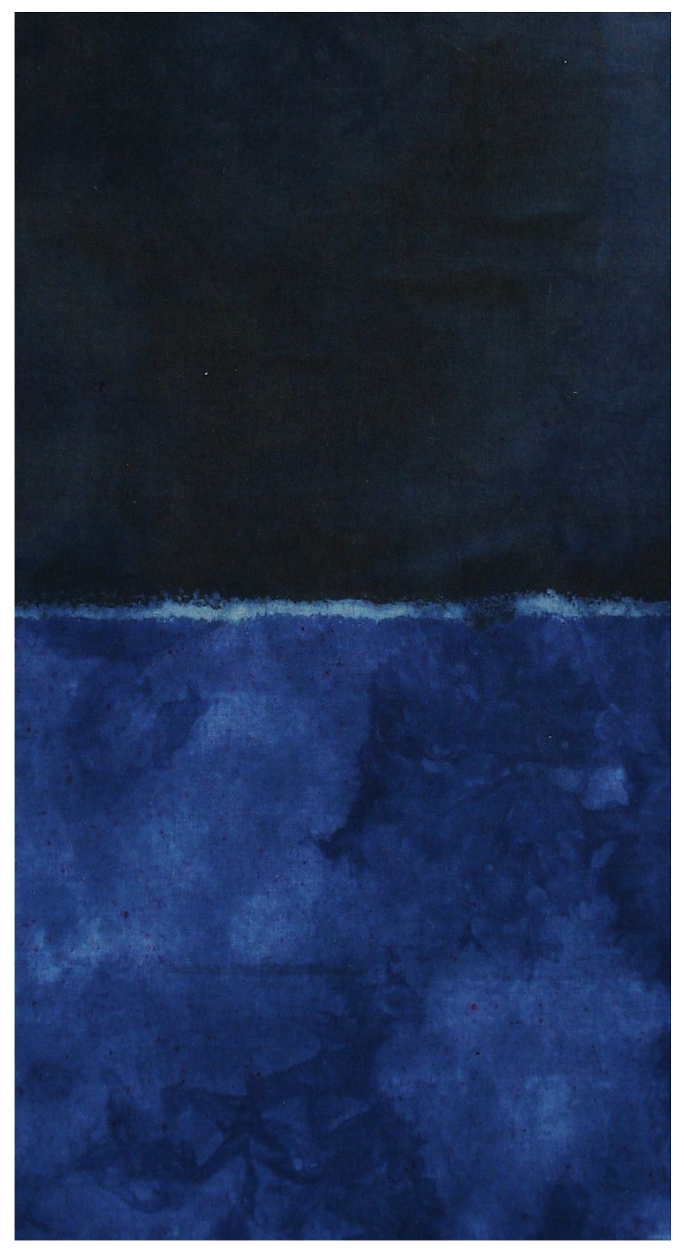
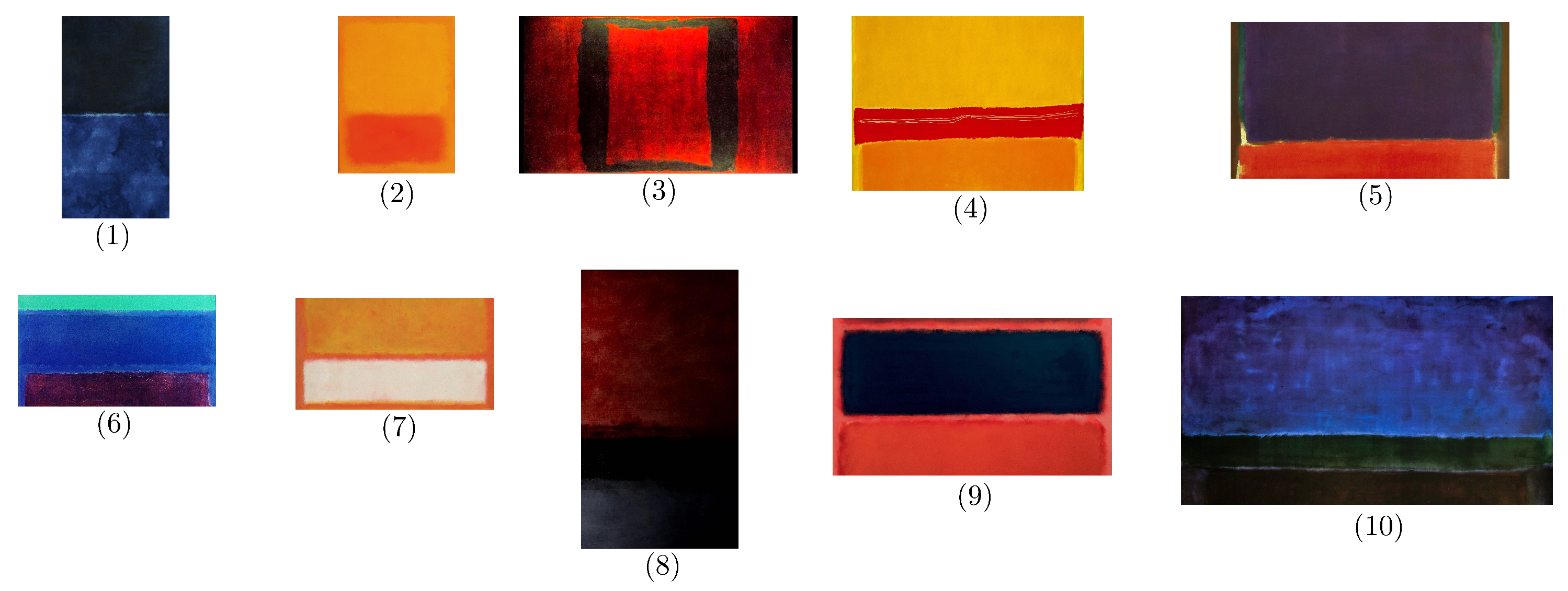
We propose a mathematical model that can reveal the hidden details, as a case for Mark Rothko’s artworks. Our result would be first demonstrated on Figure 1, and then we explore the model’s performance for each of Rothko’s artworks given in Figure 2. The desired model needs to satisfy the function ${\mathbb{Z}}_{256}^3\to {\mathbb{Z}}_{256}^3$; it also needs to increase the distance between similar color pixels, which the human eye struggles to recognize the difference between, in a way that does not ruin the entire image. That led us to the quaternion ring $\mathbb{H}$ (see expression (2)), which is a set of transformations ${\mathbb{R}}^4\to {\mathbb{R}}^4$ with specific relations. It turns out that this structure of quaternions has been applied to various fields. In [10], unit graphs of symmetric, quaternion and Heisenberg groups were studied, and in [11], a public key authentication scheme over quaternions was introduced.

The use of quaternions to represent pixels was previously considered in [12,13,14], which allows for consideration of the color information in a holistic and integrated fashion.

In this manuscript, we use the quaternion algebraic structure for pattern recognition. Our motivation is to distinguish between small color differences, which can be significant in various applications, from satellite imaging to discovering new details in a given artwork.

Our procedure can differentiate between colors that might seem identical to the naked eye but are different. Our procedure obtains an RGB image in which some colors may be similar. We transform this image using the same location for every pixel and a new color with the desired quaternion transformation, which reveals new details in the image. Lastly, our transformation can be evaluated by comparing the number of connected components using algorithms before and after the transformation (as in [15,16]).

In our case study of Rothko’s artworks, we believe that people familiar with his artworks will be surprised by the myriad of details that can be extracted from them. We believe that our method can provide a novel perspective of images that are typically considered to be straightforward.

2. Preliminaries

In this work, we use ${\mathbb{Z}}_{256}$, which is a set of the residues modulo 256; that is, $R=\left\{0,\dots ,255\right\}$, where the addition and multiplication are defined as follows

$$\begin{array}{c}\hfill \forall a,b\in R:a+b=(a+b)mod256,a·b=(a·b)mod256.\end{array}$$

(1)

This number $n=256$ can be replaced with any other finite number n, which leads to ${\mathbb{Z}}_n$. Since, in this manuscript, we would like to explore the color space, we chose $n=256$.

The Quaternion ring is defined as follows:

$$\begin{array}{c}\hfill \mathbb{H}:=\{a+b·i+c·j+d·k:a,b,c,d\in \mathbb{R}\},\end{array}$$

(2)

satisfying the relations $i^2=j^2=k^2=-1$ and $i·j·k=-1$. These relations imply $i·j=-j·i=k$, $j·k=-k·j=i$ and $k·i=-i·k=j$. We use the quaternion ring to define our RGB patterns. The quaternion ring is a generalization of $\mathbb{C}$ and can be thought of as a specific set of transformations from ${\mathbb{R}}^4\to {\mathbb{R}}^4$. We can think of the elements of the ring as vectors of the shape $(x,y,z,w)$, where each entry represents a color channel. In RGB, we only need three channels, so we will eliminate one of the entries.

This new structure is not commutative in the sense that if you take two elements, $x,y$, in $\mathbb{H}$, it is not true that $x·y\ne y·x$. For example, if we take $x=i$, which is represented by the vector $(0,1,0,0)$, and $y=j$, which is represented by the vector $(0,0,1,0)$, we will get that $x·y$ is the vector $(0,0,0,1)$, while $y·x$ is the vector $(0,0,0,-1)$ (which by the modulo is an opposite color).

In our method, we also need to evaluate the performance of our transformation, which leads us to the following definition.

Connected components labeling is a fundamental image-processing technique used to identify and differentiate objects in a digital image. It involves analyzing the pixels of an image to determine which pixels are connected and thus form individual objects. Then, assigning a unique label to each object. Connected components’ labeling begins by examining the pixels of an image and assigning a unique label to each object. This can be achieved by examining each pixel in the image, and assigning a label to each connected region of pixels. For example, a label might be assigned to each region of pixels that form a shape, or to each region of pixels with a certain color or shade. Once all the objects in the image have been labeled, the connected components’ labeling algorithm can be used to identify and differentiate between the objects in the image. This is achieved by examining the labels of the pixels and comparing them to the labels of the other pixels in the image. If two pixels have the same label, they are considered to be part of the same object. By examining the labels, the connected components’ labeling algorithm can identify the objects in the image and differentiate them from each other.

Otsu’s algorithm [17] is an algorithm in image processing used to automatically classify a given image into two (or more) classes, often referred to as the foreground and background. The algorithm is based on the idea of maximizing the interclass variance between the two classes and works by calculating the interclass variance of each possible threshold level and then selecting the threshold that maximizes the variance. The resulting threshold is then used to separate the image into two classes, with pixels within the threshold range belonging to the foreground class and those outside the range belonging to the background class. Otsu’s algorithm is widely used in image segmentation and feature extraction, as it can quickly and accurately separate an image into distinct regions. Additionally, the algorithm is often used in the preprocessing of images for applications such as facial recognition, object detection, and medical imaging.

Remark 1.

Notice that the Otsu filter can be beneficial in revealing new details in grayscale images through the selection of appropriate parameters in edge detection; however, our technique generalizes this to the RGB format.

3. Our Results

The human eye is usually unable to discern the differences between colors such as $(0,0,255)$ and $(0,0,252)$, which are both very similar blue colors. When an image is composed of such pixels, it appears to be a single-hued image. The primary objective of the manuscript is to distinguish areas with similar colors in $(R,G,B)$ format by a transformation T, which increases the distance between similar pixels in a given sub-image. For example, given two neighborhoods, $n_i$ and $n_j$, which are located relatively close to each other and similar in their $(R,G,B)$ color definition, T can transform them to the same location but yield a better color separation (as we will show and explain later on in

Table 1. This is a sample of the change between the output and input, which reveal hidden layers in the painting. (a) Original input image before applying the transformation. (b) Output after applying the transformation obtained by $\mathbb{H}·(2+i+3j)$, after eliminating the second vector component.

(a)
	662	663	664	665	666
230	[30 38 49]	[31 39 50]	[28 38 50]	[31 41 53]	[32 42 54]
231	[30 38 49]	[31 39 50]	[28 38 50]	[31 41 53]	[32 42 54]
232	[30 38 49]	[31 39 50]	[28 38 50]	[31 41 53]	[32 42 54]
233	[30 38 49]	[31 39 50]	[28 38 50]	[31 41 53]	[32 42 54]
234	[30 38 49]	[31 39 50]	[28 38 50]	[31 41 53]	[32 42 54]
(b)
	662	663	664	665	666
230	[210 3 124]	[208 9 128]	[214 5 116]	[208 23 128]	[206 29 132]
231	[210 3 124]	[208 9 128]	[214 5 116]	[208 23 128]	[206 29 132]
232	[210 3 124]	[208 9 128]	[214 5 116]	[208 23 128]	[206 29 132]
233	[210 3 124]	[208 9 128]	[214 5 116]	[208 23 128]	[206 29 132]
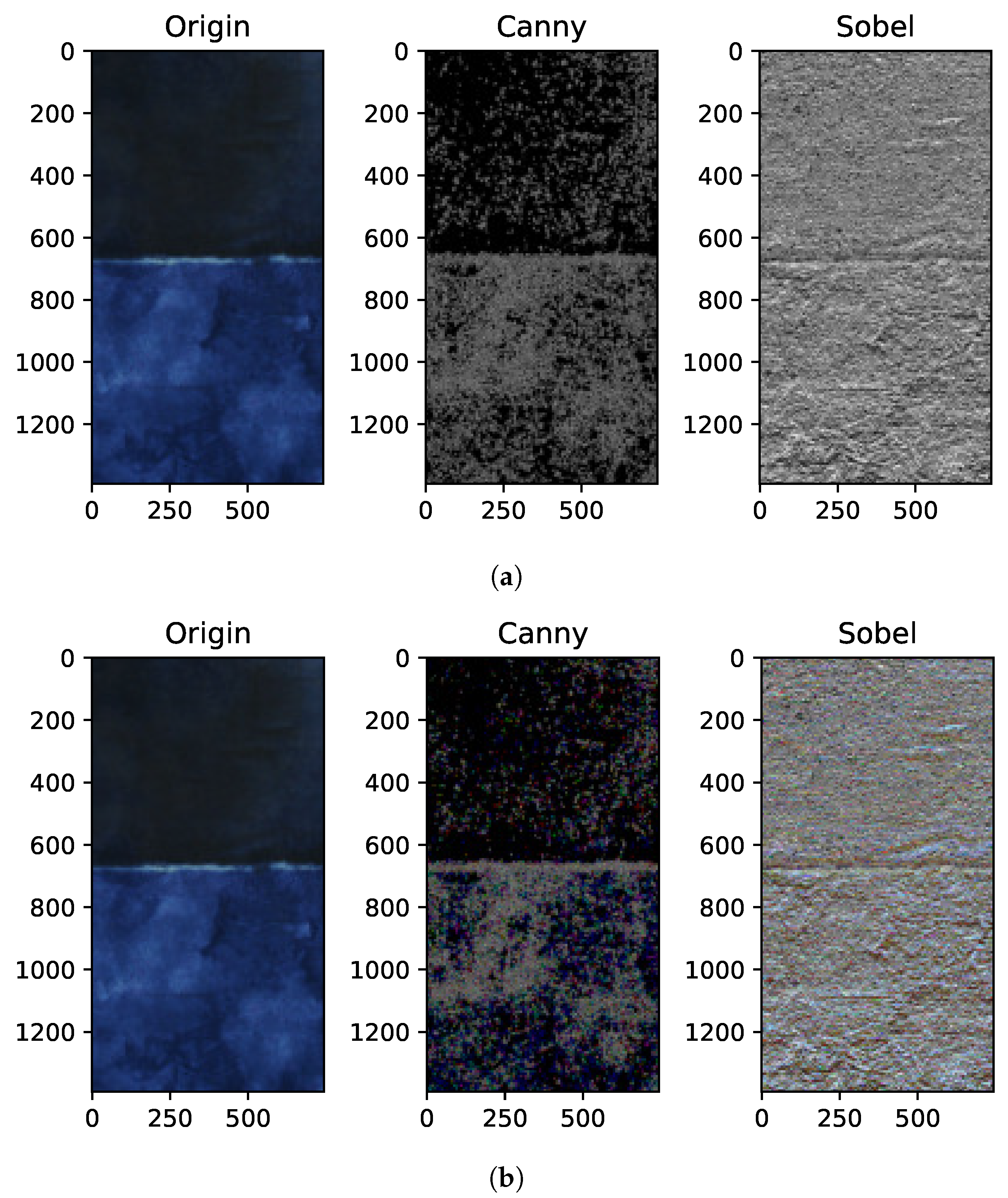
234	[210 3 124]	[208 9 128]	[214 5 116]	[208 23 128]	[206 29 132]

). This characterization can highlight nuances that may seem esoteric, yet are of great importance in certain image-processing applications. We are confident that our technique can successfully perform this kind of separation, whereas common filters based on gradient techniques (see the comparison in Figure 3) often have difficulty recognizing differences in colors in a given location neighborhood.

Figure 1 presents a typical Rothko artwork, characterized by visual simplicity, a limited number of colors, and its acclaimed rectangular shapes. This manuscript uses Rothko’s artworks as a case study to meet the requirements of the problem, which involves distinguishing between similar colors within an image. To accomplish this, we employ the Quaternion ring, which is a map ${\mathbb{R}}^4\to {\mathbb{R}}^4$ that needs to be matched to a transformation on the RGB color space, i.e., ${\mathbb{Z}}_{256}^3\to {\mathbb{Z}}_{256}^3$. To separate similar pixels, such as $p_1=(0,0,255)$ and $p_2=(0,0,252)$, we define a function that transforms them such that the distance $d(p_1,p_2)\ll d(\widetilde{p_1},\widetilde{p_2})$, where $\widetilde{p_1},\widetilde{p_2}$ are the pixels after the transformation.

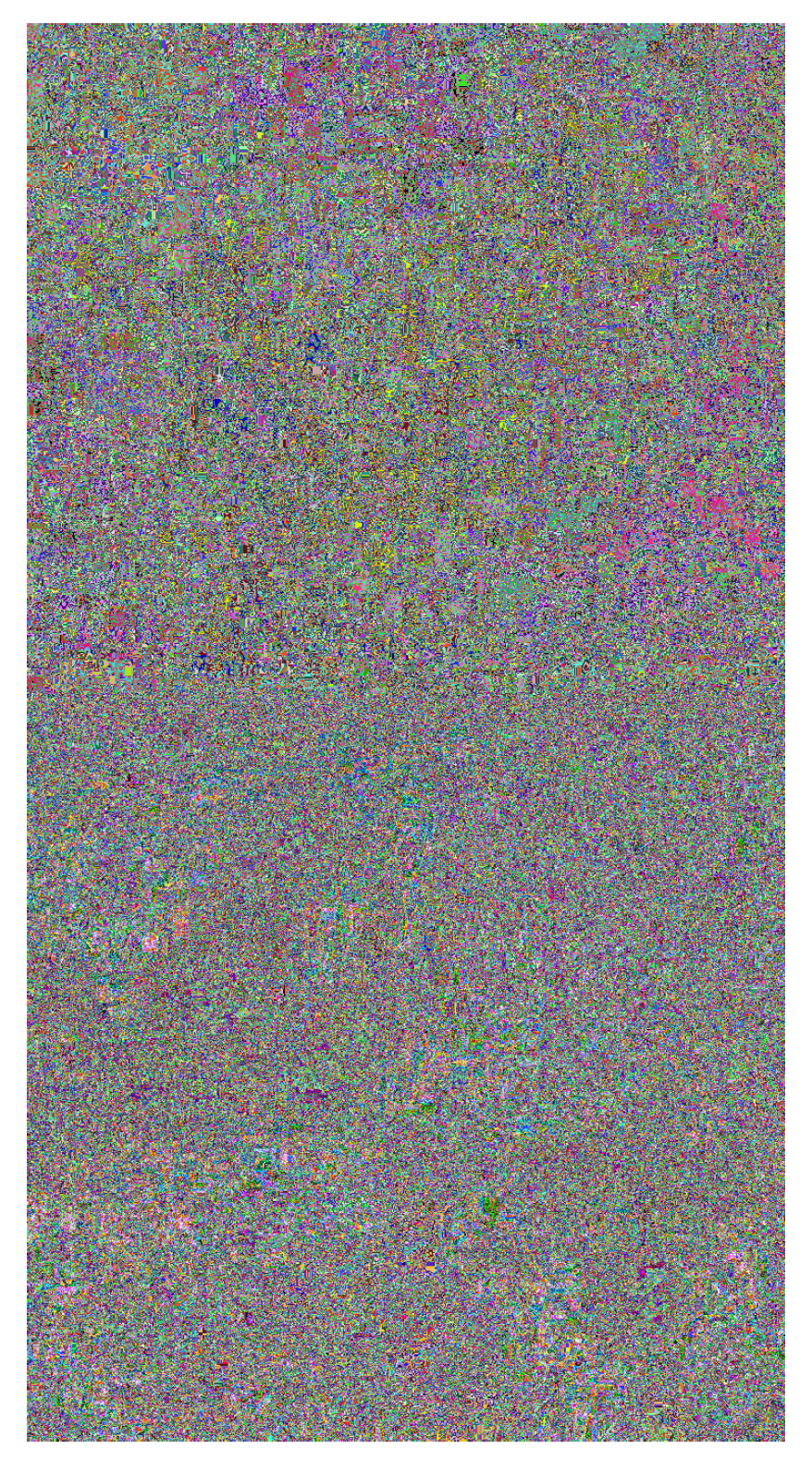
Our technique is based on the given algebraic structure, which, with the right function, can reveal separation. Care must be taken with the transformation of the pixels: if $d(p_1,p_2)=d(\widetilde{p_1},\widetilde{p_2})+\epsilon$ (where $\epsilon$ is a small integer), the hidden parts of the image will not appear if the transformation is not significant enough from the original. Conversely, if the pixel transformation results in too large of a distance between every two neighbors, the image will become chaotic, as shown in Figure 4. This image was obtained by a transformation, which significantly increases the metric between neighboring pixels and transforms the pixels to ‘far’ in the color space (compared to the original Figure 1); in this case, it is defined by ${\mathbb{H}}^2$, resulting in a noisy image.

To succeed in this separation, trial and error are key to discovering the appropriate distance, which reveals areas with distinct color differences, leading to the completion of the clustering process. Ultimately, our results will be measured by the number of clusters in the image before and after transforming the neighboring structure in the given color space.

Notice that multiplication by quaternions, such as $i·\mathbb{H}⟹\left|i·\mathbb{H}\right|=\left|\mathbb{H}\right|$, will not lead to the desired result, since it only changes the colors, but $d(p_1,p_2)=d(\widetilde{p_1},\widetilde{p_2})$. We are now ready to apply our method to reveal hidden details.

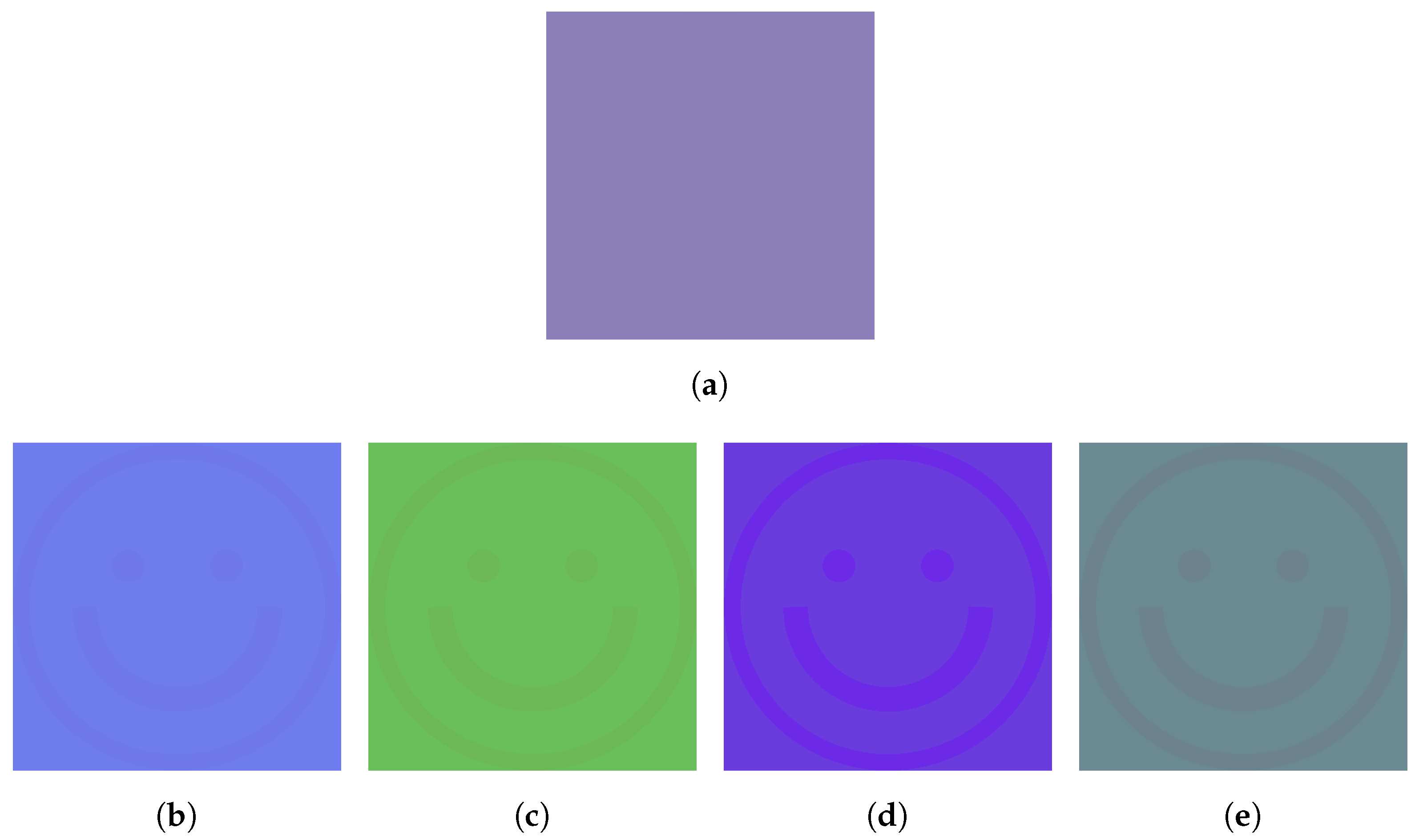
3.1. Find the Hidden Details

Figure 5a shows a solid color image; however, upon closer inspection, there are a few small changes compared to an absolute solid color image. Some of the pixels are defined by an arbitrary color in RGB; let this color be $(r,g,b)$, and some by $(r+1,g+1,b+1)$, which are too subtle for the human eye to detect. We choose the quaternion transformation obtained by $\mathbb{H}·(2+i+3j)$, which leads to

$$\begin{array}{c}(a+b·i+c·j+d·k)·(2+i+3j)\hfill \\ \hfill =(2a-b-3c)+(a+2b-3d)·i+(3a+2c+d)·j+(3b-c+2d)·k\end{array}$$

which is equivalent to the vector $(2a-b-3c,a+2b-3d,3a+2c+d,3b-c+2d)$. Figure 5b–e are obtained by nullifying the first, second, third, and fourth elements of the vector, respectively. This result is obtained by increasing the distances between neighboring pixels, thus revealing the smiley in the image (see further details in the following Section 3.2).

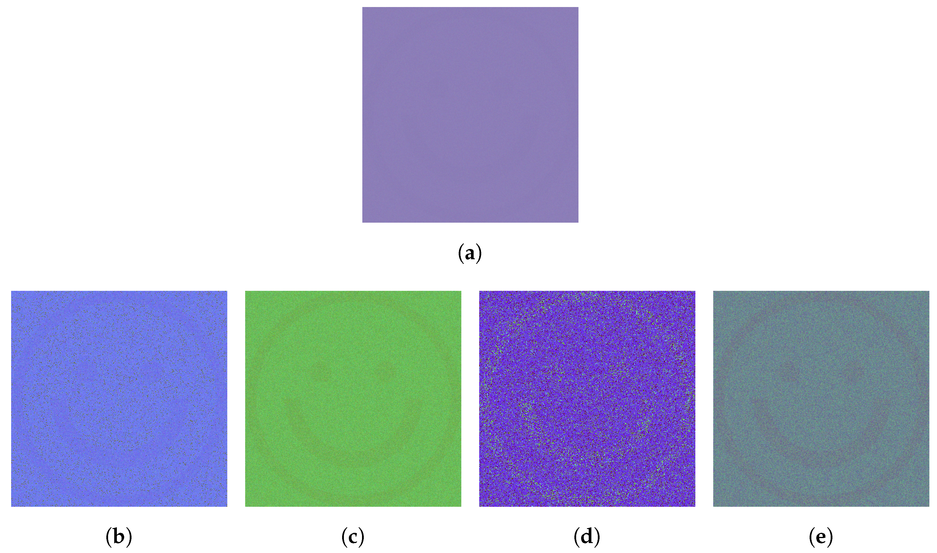
Note that this technique works as expected when adding random noise to the image, see Figure 6.

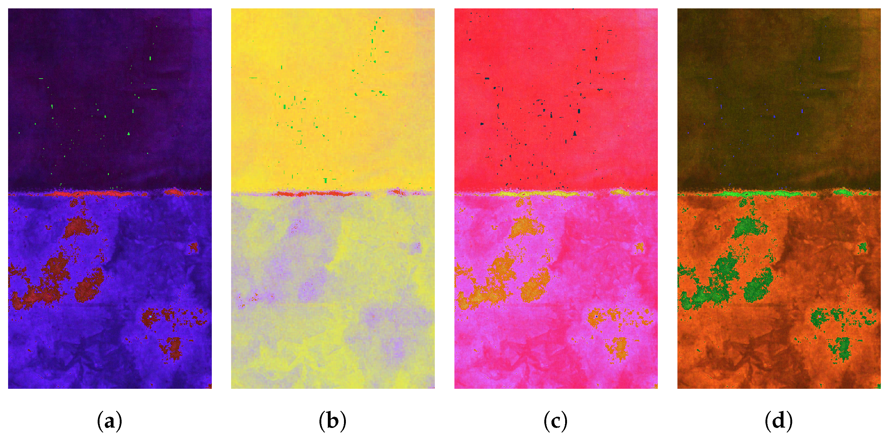
3.2. Demonstrating Our Technique on Rothko’s Artwork No. 1

In this subsection, we explore different quaternion transformations of Rothko’s artwork in Figure 1. These different multiplication transformations lead to vastly different results. We will now describe each of them.

Firstly, consider the multiplication transformation

$$\mathbb{H}·(1+k)=(a-d,b+c,-b+c,a+d)\in {\mathbb{R}}^4.$$

This transformation increases the Euclidean distance by between $\mathbb{H}$ and $\mathbb{H}·(1+k)$ by $\sqrt{2}$, which is our initial choice of increasing distances between neighboring pixels. To reduce the dimension to represent an RGB image, one of the vector components must be eliminated. As an example, consider the fourth component $a+d=0$, which leads to $(2a,b+c,-b+c)$. Now, since the desired output is an RGB image, we choose $R=a$, $G=b$, and $B=c$, i.e., $(2R,G+B,B-G)$ where we apply modulo 256 on each channel, see Figure 7d. In a similar way, Figure 7a is obtained by eliminating the first component by the rule $a-d=0$, Figure 7b is obtained by eliminating the second component by the rule $b+c=0$, and Figure 7c is obtained by eliminating the third component by the rule $-b+c=0$. Notice that by multiplying from the left, we obtain the vector $(a-d,b-c,b+c,a+d)$.

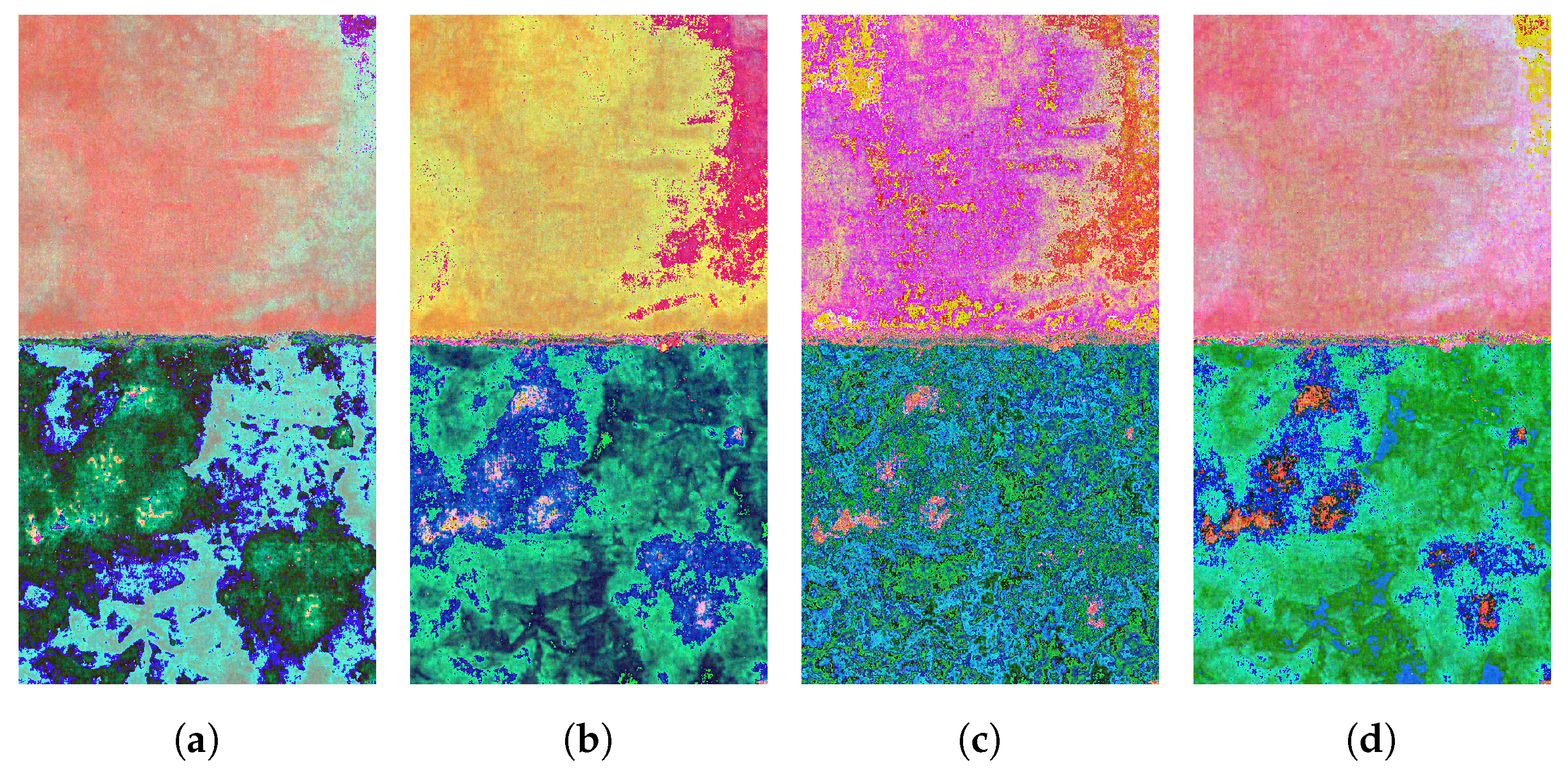
Secondly, consider the multiplication transformation $\mathbb{H}·(2+i+3j)=(2a-b-3c,$$a+2b-3d,3a+2c+d,3b-c+2d)\in {\mathbb{R}}^4$. This transformation increases the distance between $\mathbb{H}$ and $\mathbb{H}·(2+i+3j)$ by $\sqrt{12}=2\sqrt{3}$, which is larger than the previous transformation due to our expectation that it should be increased (a justification will be given in the next Section 4). In a similar manner, we reduce the amount of vector components from four to three, which leads to Figure 8. Table 1 compares between an area in the source image and the transformed image. We explore the location $(i,j)\in {\mathbb{N}}^2$ of the images where $i\in [230,234]$ and $j\in [662,666]$, which define a color $pixel(i,j)$. As we can observe from the source image, neighboring pixels are relatively close in the color space. However, in the transformed image, there is a marked contrast between them, which subsequently leads to better color separation.

Note that every quaternion polynomial from degree $\ge 2$ leads to a chaotic image, as in Figure 4.

4. Estimations and Comparison for Measuring the Quaternion Transformation Performance

Despite the similar number of colors in the source and transformed images, we must provide a quantitative measure to verify the presence of greater visual detail in the transformed image. These visual details are obtained through the quaternion transformation, which leads to a sharp color change in the vicinity of a given pixel in the transformed image. This sharp color change creates different color areas, which can be thought of as different connected components. We evaluate our procedure by the number of connected components; that is, a comparison between the number of connected component labeling in the source image and the transformed image, which was obtained by the Quaternion transformation. Our procedure for the estimation is as follows: The given image is converted to grayscale, then a threshold mask is obtained using Otsu’s method, which outputs a black-and-white image to which we apply the connected component labeling algorithm (in our case, we chose the Spaghetti Labeling algorithm), and return the number of connected components.

This procedure was applied to ten images of Rothko; the results are presented in

Table 2. Connected components before and after the transformation for each image in the dataset, after eliminating the fourth vector component of the transformation output. (a) The comparison is for the transformation obtained by $\mathbb{H}·(1+k)$. (b) The comparison is for the transformation obtained by $\mathbb{H}·(2+i+3j)$.

(a)				(b)
Image	Original	Final	Factor	Image	Original	Final	Factor
1	1593	2566	1.610797	1	1593	4536	2.847458
2	571	923	1.616462	2	571	1141	1.998249
3	1484	3555	2.395553	3	1484	6441	4.340296
4	34	3873	113.911765	4	34	16,996	499.882353
5	3706	4774	1.288181	5	3706	14,814	3.997302
6	891	8366	9.389450	6	891	31,276	35.102132
7	339	565	1.666667	7	339	8593	25.348083
8	602	163	0.270764	8	602	1687	2.802326
9	325	4396	13.526154	9	325	10,713	32.963077
10	4040	5600	1.386139	10	4040	11,461	2.836881

a,b, which compares the number of connected components before and after applying a given quaternion transformation. This indicates a lower bound of a factor of 2 for Rothko’s No. 2 artwork in the dataset and an upper bound of almost 500.

5. Summary

This manuscript presents a quantitative measure to verify the presence of greater visual detail in images of Rothko using a quaternion transformation. A procedure was carried out to compare the number of connected components before and after the quaternion transformation. We defined a performance metric as the ratio between the connected components after and before the transformation. The results demonstrate a lower bound of a factor of two and an upper bound of almost 500, indicating a significant difference in visual detail between the source and transformed images.